Article

Rapid Determination of Wood and Rice Husk Pellets’ Proximate Analysis and Heating Value

1
College of Biosystems Engineering and Food Science, Zhejiang University, 866 Yuhangtang Road, Hangzhou 310058, China
2
Key Laboratory of Spectroscopy Sensing, Ministry of Agriculture, Hangzhou 310058, China
3
The Rural Development Academy, Zhejiang University, 866 Yuhangtang Road, Hangzhou 310058, China
4
State Key Laboratory of Modern Optical Instrumentation, College of Optical Science and Engineering, Zhejiang University, 866 Yuhangtang Road, Hangzhou 310058, China
*
Authors to whom correspondence should be addressed.
Energies 2020, 13(14), 3741; https://doi.org/10.3390/en13143741
Submission received: 24 June 2020 / Revised: 11 July 2020 / Accepted: 15 July 2020 / Published: 20 July 2020
(This article belongs to the Special Issue Advanced Technologies for Biomass)

Abstract

:
Biomass pellets are a potential renewable and clean energy source. With the advantages of perfect combustion performance and easy storage and transport, biomass pellets have gradually replaced fossil fuels and become widely used. Rapid and accurate determination of biomass pellets’ quality is critical to efficient energy use. Laser-induced breakdown spectroscopy (LIBS) combined with chemometric methods were utilized. The gross calorific value (CV) and ash content (Ash), volatile matter (VM) and fixed carbon (FC) were firstly measured and analyzed. LIBS spectra and their corresponding elements of biomass pellet samples were analyzed. Three quantitative analysis models for quality indexes including partial least-squares regression (PLSR), least squares-support vector machines (LS-SVM), extreme learning machines (ELM) were further built. All models performed well, especially the LS-SVM model which obtained the best determination results, with all R2 values over 0.95. Concurrently, the modeling performance of ash was slightly better than that of the other three quality indexes, which further confirmed the feasibility of using relevant elements to predict biomass quality indexes. The overall results indicated that LIBS coupled with suitable chemometrics could be an alternative promising method to determine quality indexes of biomass pellets and further improve energy utilization by using biomass materials with better quality.

Graphical Abstract

1. Introduction

The energy crisis is one of the greatest challenges that our society is facing nowadays, so it is essential to develop sustainable new energy resources to reduce the use of fossil fuels. In recent years, biomass energy has drawn wide attention around the world as a clean and renewable energy source [1,2]. Especially for biomass pellets there is a growing market demand [3], since have the advantages of a high combustion efficiency, convenient storage and transport, environmental friendliness and low cost [4,5]. In order to make full use of this biomass energy source, it is important to analyze the combustion performance of the biomass pellets. Industrial analysis components including carbon content, volatile matter content and ash content are all important factors affecting biomass combustion performance [6,7,8,9]. The calorific value is a direct indicator of biomass combustion performance [10,11]. Thus, accurate and fast determination of all these quality indexes are of great importance in the efficient utilization of energy. Traditional detection methods are mainly industrial technology and chemical analysis, and detection methods of different indexes are different. It is time, cost, and labor-consuming to measure all these indexes simultaneously [12]. Therefore, it is particularly necessary to develop newly rapid quantitative analysis techniques.
Laser-induced breakdown spectroscopy (LIBS) is a recently emerged spectroscopic technique based on elemental analysis [13]. It provides a reliable alternative for qualitative and quantitative analysis of the composition of samples [14,15]. With the merits of fast detection, little sample or no pretreatment, multi-elemental simultaneous detection capability, LIBS has been widely applied to sample analysis in many fields ranging from agriculture and biological to industry [16,17,18,19]. In recent years, there have been many researches on energy using LIBS. Li et al. [20] built a PLS quantitative prediction model for the calorific value of coal based on LIBS combined with different spectral pre-processing methods. The best result was achieved when using the 11 points smoothing combined with the second-order derivation, with both the correlation coefficient of calibration set and correlation coefficient above 99%. Yao et al. [21] used artificial neural networks to quantitatively analyze the ash, volatile matter, fixed carbon, and gross calorific value of coal, and a reliable and accurate result was achieved, with the correlation coefficients of all prediction models above 97%. Dong et al. [22] employed LIBS and multiple linear regression combined with the partial least squares regression (PLSR) and support vector regression (SVR) to analyzed the carbon contents in coal samples. The best results of carbon calibration were obtained using LIBS coupled with an MLR model-added SVR correction. The determination coefficient (R2), root mean standard error of cross validation (RMSECV) and root mean standard error of prediction (RMSEP) were 0.99%, 0.00039%, and 1.43%, respectively. AINTS et al. [23] focused on the quantitative assessment of the calorific value of Estonian oil shale using LIBS. The ordinary multivariate regression analysis was applied, and the correlation coefficients of the prediction model for the calorific value and moisture content were above 90% and 75%, respectively. Lu et al. [24] investigated the feasibility of using LIBS to determine gross calorific value, carbon content, volatile matter content and ash content. Several pre-processing methods combined with PLS model were used, and it was turned out that the PLS model based on spectra that combined baseline correction with Z-score standardization performed best, with the coefficient of determination of all prediction models above 96%. To the best of our knowledge, there are no studies focused on quantitative prediction of biomass fuels properties using LIBS combined with different chemometrics.
Based on the abovementioned situation, the objective of this study was: (1) to explore the feasibility and accuracy of using LIBS to analyze the properties of biomass pellets; (2) to select important spectral lines for building the relationships between the important elemental emission lines and quality indexes; and (3) to build accurate and reliable prediction models for the quality indexes of biomass pellets.

2. Materials and Methods

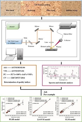
2.1. Sample Preparation

The biomass pellets were provided by different bioenergy companies, and they are representative of the most commonly used varieties found on the biofuel market in China. They mainly included rice husks, pine wood, rubber wood, and red wood. The distance between the sample surface and the lens for laser focusing will affect the intensity of the spectral signals. Besides, uneven samples will also cause interference in the spectral signals. Thus, a uniform and regularly shaped sample is of great importance. In order to obtain accurate and reliable experimental data, the biomass pellets were first milled and then compressed into a circle tablet using a pressing machine (FY-24, SCJS, Tianjin, China) for 30 s and under a pressure of 10 MPa. The resulting side length and thickness were 10 mm and 2 mm, respectively. The tablets were then dried at 60 °C for 6 h in an oven. A total of 128 tablets samples were prepared. They were divided into calibration and prediction sets in a ratio of 3:1 by joint x–y distances (SPXY) methods [25]. Thus, 96 samples and 32 samples were obtained for calibration and prediction, respectively. Besides, the four kinds of biomass pellets were distributed in both calibration and prediction sets to make the analyses more reliable.

2.2. Determination of Quality Indexes

In this study, industrial analysis components were also determined according to the traditional methods. Ash content (Ash) and volatile matter (VM) were measured according to ASTM D1102-84 and ASTM E872-82 [26]. The gross calorific value (CV) (MJ·kg−1) was determined in accordance with the China national standards GB/T30727-2014 using an oxygen bomb calorimeter (5E-AC, Chansha Kaiyuan Instrument Co., Ltd., Changsha, China). Fixed carbon (FC) was calculated after determining the Ash and VM content according to the following equation:
FC% = 100% − Ash% − VM%
The values of Ash, VM, and FC were dry basis.

2.3. Experimental Apparatus and LIBS Measurement

A self-built LIBS system (Figure 1) was used in this work. It mainly comprised of a Q-switched Nd:YAG pulsed laser (Vlite-200, Beamtech Optronics, Beijing, China) with the maximal energy of 200 mJ @532 nm for generating laser pulse to ablate samples, an Echelle spectrograph (ME5000, Andor Technology, Belfast, UK) equipped with an (intensified charge coupled device) ICCD camera (iStar DH340T, Andor Technology, Belfast, UK) for collecting spectral signals, and a digital delay pulse generator (DG645, Stanford Research Systems, San Jose, CA, USA) for controlling the delay time between the laser and the ICCD camera. In addition, lens, mirrors and X-Y-Z stage were used for laser transmission and sample placement. A Hg: Ar lamp (HG-1, Ocean Optics, Winter Park, FL, USA) and a Deuterium Halogen light source (DH-2000-BAL-CAL, Ocean Optics, Winter Park, FL, USA) were used for the calibration of the wavelength and intensity. Experimental parameters were optimized by the response surface methodology (RSM) to obtain a best signal to noise ratio (SNR) and relative standard deviation (RSD). Based on the optimization, the energy of laser pulse was 60 mJ with 1 Hz repetition rate, the delay time was 1.5 μs, and the gate width of ICCD was 10 μs. Besides, the distance between the lens and sample surface was optimized to 98 mm when a good spectral signal was obtained.
LIBS measurements were conducted after setting the parameters. First, the laser beam was adjusted to be focused 2 mm below the sample surface to avoid any interference caused by an uneven sample surface. The signal detector was then adjusted to ensure that the spectral signal could be collected. After that, a total of 80 spectra of each sample were obtained by controlling the moving path of the X-Y-Z stage. 16 position of each tablet sample were ablated with five successive accumulations. At last, the average of 80 spectra was used to be the spectrum of the sample.

2.4. Data Pretreatment and Analyze

In order to eliminate the impact caused by experimental instruments and radiation generated by plasma formation, and further to improve the precision and repeatability of LIBS detection, several pre-processing methods were introduced, including baseline correction, wavelet transform, normalization, and outlier discarding. Baseline correction could eliminate background signals, and wavelet transform could reduce any noise. Normalization could effectively reduce the fluctuation of each shot and improve signal stability. Detailed information of these methods were mentioned in our previous work [27]. Outlier discarding could improve the reliability and accuracy of the data. A self-developed outlier removing algorithm based on median absolute deviation (MAD) was used in this work. In order to meet our particular demands, a relatively stable spectral line of CN 388.29 nm was applied to identify outliers. Once the difference between the intensity and median of CN 388.29 nm exceeded 2.5 times the MAD, the spectrum would be considered as an outlier and be removed. Outliers removing was repeated until there were no outliers or a maximum of 25% of the original spectra were removed.

2.5. Chemometrics for Data Analyze

Several chemometric methods were conducted after data pretreatment, including partial least squares regression (PLSR), least squares-support vector machines (LS-SVM), extreme learning machines (ELM). The specific procedure of LIBS data analysis is shown in Figure 2.
Partial least-squares regression (PLSR) is a widely used linear analysis algorithm for the quantitative analysis of large datasets, especially for spectra [28,29,30,31]. The main principle of this method is to convert the large linear original data into independent latent variables which still contain most of the information of the original variables, and the first few important latent variables will be used for further analysis [32,33]. In this work, PLSR models were applied based on the value of the biomass pellets’ quality indexes and the intensities of LIBS spectrum. Full cross-validation was used to reduce the possibility of overfitting of models. Besides, the number of latent variables is also important for modeling, and it was determined when the minimal mean squared error was obtained [34].
Different from PLSR, the least-squares support vector machine (LS-SVM) is a commonly used non-linear machine learning method that can be used to deal with both linear and non-linear problems [35,36,37,38]. It has been turned out to be a good choice for quantitative analyses for a small dataset [39,40]. According to the previous study, kernel function and its parameters including sig2 and gam have a great influence on the performance of the LS-SVM model. Kernel function is the formula that maps complex data to high-dimensional space for linear calculation. The parameter sig2 reflects the complexity of the sample distribution in the feature space. The parameter gam was used to control the fitting error of the function. These two parameters together determine the generalization ability and training error of the function [41]. In this case, radial basis function (RBF) was adopted as a kernel function due to the advantage of good generalization ability. Then we optimized sig2 and gam when the minimum value of RMSECV was obtained in the grid-search within the range of 103–1010. Besides, full cross-validation was also used as the same as that in PLSR models. The whole process was conducted in MatLab.
Extreme learning machine (ELM) is a recently developed machine learning algorithm based on single-hidden layer feedforward neural networks (SLFNN), and it runs in a simpler and easier way than traditional neural network methods [42,43]. Output weights can be obtained by randomly initializing input weights and hidden layer biases in global optimization [44,45]. In particular the number of hidden layer biases is obtained by continuous optimization in a predefined range which is usually less than the number of samples for modeling. This property makes ELM runs significantly faster with guaranteed learning accuracy. Besides, it has the advantage of good generalization performance [46] which makes it suitable for both quantitative and qualitative analysis. In this case, we tried to explore the feasibility of quantitative prediction for the quality indexes of the biomass pellet.
In addition, performances of all the abovementioned models were evaluated by several indicators, including the coefficient of determination in calibration and prediction sets (R2C and R2P), root mean square error (RMSEC and RMSEP). R2 reflects the relationship between the predicted value of the quality indexes of biomass pellet and their reference value, RMSE reflect the prediction error of the model. The closer the R2 to 1, the smaller the RMSE, the better the model will perform.

3. Results and Discussion

3.1. Quality Indexes Statistics

The descriptive statistics of the quality indexes for all samples are listed in Table 1. Due to the effect of types and processing methods, the quality indexes of the biomass pellets are totally different. It is obvious that VM took up a large proportion in all components, which varied from 74.96% to 88.99%. FC followed, varying from 10.39% to 21.22%. The Ash contents were in the range of 0.26% to 15.94%. CV varied in the range of 15.1 to 19.54 (MJ·kg−1). These ranges provide the foundation for developing reliable quantitative prediction models of the quality indexes.
In order to more comprehensively evaluate the quality of biomass pellets, we have explored the internal relationships of these quality indexes. Table 2 shows the Pearson’s correlation coefficients among the quality indexes of 128 biomass pellets. It can be clearly seen that CV was significantly positively related to VM, with correlation coefficients of 0.751. It also had a significant negative correlation with Ash, and the correlation coefficients was −0.903. Besides, Ash and VM were significantly negatively correlated. FC has a positive correlation with Ash and a negative correlation with VM, but there is no significant correlation with CV. These results were also roughly consistent with previous research [12,47]. These results also indicated that the higher the value of VM is, the lower the value of Ash is, and the higher the value of CV will be, which further lead to a better combustion performance of the biomass pellets.

3.2. Spectral Analysis

The spectra of the four different types of biomass pellets (Figure 3) were used as examples. To eliminate the effects of noise, only spectra of 280.25–854.12 nm (18354 variables) were used for the analyses. Based on previous research and the National Institute of Standards and Technology (NIST) database, the specific elements and molecular bands corresponding to the spectral lines were given in Figure 3. These emissions included O (777.19 nm, 844.63 nm), N (742.36 nm), K (766.49 nm, 769.89 nm), Ca (393.39 nm, 422.67 nm, 445.47 nm, 616.21 nm), Na (588.99 nm, 819.48 nm), Mg (280.27 nm, 285.21 nm), Al (309.27 nm), Fe (373.48 nm, 374.94 nm), Mn (403.07 nm), Si (288.15 nm, 390.5 nm), Ti (319.19 nm), C2 (516.52 nm), CN (388.32 nm) etc. According to previous research, these elements have direct effects on the quality indexes. Metal oxides formed from the elements K, Ca, Na, Mg, Al, Fe, Mn, Si, Ti, are the main constituents of ash [48,49,50]. The main constituents of VM including CO2, NO2, CO, = etc were also formed from elements C, O and N [51,52,53]. FC was also directly related to the element C and molecular bands of C2 and CN [24,54]. Besides, all elements affected each other due to the ionization and the combination of elements in the process of compound formation [55]. Therefore, there should have a good correspondence between these quality indexes and the elements. In addition, CV was highly affected by Ash and VM as mentioned before. Thus, the value of CV could also predicted by the content of these elements. It could also be clearly observed from Figure 3 that the elements in different samples are consistent, but the contents of the elements were different. This further indicated the possibility of predicting these the quality indexes using the contents of the elements. Therefore, chemometric models based on the spectral lines covered these elements were further built to predict the value of the quality indexes quantitatively.

3.3. Prediction of Quality Indexes

PLSR, LS-SVM and ELM were applied to build the quantitative models for accurate prediction. The quantitative modeling results were stated in Table 3.
Ash is the residue left after the complete combustion of all combustibles in the biomass and the minerals undergo a series of complex reactions such as decomposition and combination. Its melting characteristics have a great influence on the combustion performance of biomass. Previous research revealed that biomass with low ash content has a better combustion performance [56,57]. Figure 4 shows the fitting results of models for Ash. It’s clear that all models performed well, with all R2 above 0.95. Especially LS-SVM gave the best result, with R2 in calibration and prediction sets reaching 0.999 and 0.977, respectively. It could be concluded that LIBS combined with chemometrics is a promising way to predict ash content and further to provide reference for evaluating the combustion performance of biomass materials.
VM refers to the gaseous product produced by the decomposition of biomass organic matter. It has a great effect on the ignition and combustion of biomass and can reflect the quality of biomass. In contrast to ash, the higher the VM content is, the better the combustion performance of the biomass will be. In this study, calibration and prediction results of models for VM are provided in Figure 5. It could be seen that all data fitted well in both calibration and prediction set. In particular, LS-SVM obtained more accurate results, with R2 in both calibration and prediction sets over 0.97. On the whole, the modeling results showed that LIBS combined with LS-SVM could be a good tool for selecting biomass with higher VM content, which might be used as a good fuel.
Fixed carbon is the residue remaining after removing moisture, Ash, and VM from biomass. The ignition point of fixed carbon is very high [58]. Generally, the higher the fixed carbon content is, the greater the temperature for ignition and combustion is [59]. Figure 6 shows the model fitting results for FC. As seen, LS-SVM performed perfect, and R2 in both calibration and prediction sets were over 0.95. ELM gave the worst results which was still acceptable, with R2 in calibration and prediction sets were 0.874 and 0.836. Thus, using LIBS and suitable chemometrics to predict the content of FC could provide a reference for selecting better biomass fuels.
CV refers to the amount of heat released per unit mass of biomass fuels when it is completely combusted. It is an important indicator for evaluating the combustion performance of biomass. Figure 7 exhibits the calibration and prediction results of CV. It can be observed that all models gave a satisfactory result, and the best model for CV determination was obtained using LSSVM (R2C and R2P were 0.993 and 0.971, respectively). Thus, fast and accurately predicting of CV by using LIBS and LS-SVM model could be conducive to industrial applications.
As a group, all models performed well for predicting these quality indexes. LS-SVM model performed best. As for the four indices, the prediction results for FC are relatively poor, it might be caused by the moisture. The biomass is extremely hydrophobic and it might quickly reabsorb some moisture although we have dried the samples, thus there might be some deviations in the determination of nominal fixed carbon content according to Equation (1). Besides, the prediction results of ash were slightly better that the other three indexes. This might be credited to the fact that that Ash was more directly related to elements, and this further indicated the capability of using LIBS to predict biomass quality.

4. Conclusions

In the present study, LIBS technology combined with three chemometric methods was adopted to determine the four quality indexes of biomass pellets. Statistics of CV and industrial analysis components including Ash, VM, FC were firstly determined using traditional methods. The internal relationships of these quality indexes were then analyzed based on these statistics. CV and VM were both negatively related to Ash and FC, and the relationships between them were significant, except for that between CV and FC. Besides, there was a significantly positive relationship between CV and VM, Ash and FC. LIBS spectra of four different kinds of samples were further analyzed, and this showed that the spectral lines corresponded to the elements that were related to the four indexes. PLSR, LS-SVM and ELM were applied to build quantitative analysis models for these quality indexes. All models showed a satisfactory prediction ability, especially LS-SVM models, with all R2 values above 0.95. Among the four indexes, the prediction accuracy of Ash was relatively better. On the whole, LIBS technology coupled with LS-SVM methods exhibited great potential in determining the quality indexes of biomass pellets. It might be developed as a good tool for fast industrial detection of biomass fuels, further improving the efficiency of energy use.

Author Contributions

X.L. and X.F. performed the measurements; X.L. wrote the manuscript; X.L., X.F., Y.H and L.H. designed the experiment; Y.H. and X.F. reviewed the initial design of the experiments and provided guidance for the writing of the manuscript; All authors have read and agreed to the published version of the manuscript.

Funding

This work was supported by the Planned Science and Technology Project of Guangdong Province, China (no. 2019B020216001), and the Project of Guangdong Province Universities and Colleges Pearl River Scholar Funded Scheme, China (no. 2016).

Conflicts of Interest

The authors declare no conflict of interest.

References

  1. Keles, S.; Kar, T.; Bahadır, A.; Kaygusuz, K. Renewable energy from woody biomass in Turkey. J. Eng. Res. Appl. Sci. 2017, 6, 652–661. [Google Scholar]
  2. David, E.; Kopac, J.; Armeanu, A.; Niculescu, V.; Sandru, C.; Badescu, V. Biomass—Alternative renewable energy source and its conversion for hydrogen rich gas production. E3S Web Conf. 2019, 122, 01001. [Google Scholar] [CrossRef]
  3. Kaygusuz, K.; Toksoy, D.; Bayramoğlu, M.M. Global utilization of wood pellet for residential heating. J. Eng. Res. Appl. Sci. 2017, 6, 688–697. [Google Scholar]
  4. Kiss, I.; Alexa, V.; Sárosi, J. Biomass from Wood Processing Industries as an Economically Viable and Environmentally Friendly Solution. Analecta Tech. Szeged. 2016, 10, 1–6. [Google Scholar] [CrossRef]
  5. Feng, X.; Yu, C.; Liu, X.; Chen, Y.; Zhen, H.; Sheng, K.; He, Y. Nondestructive and rapid determination of lignocellulose components of biofuel pellet using online hyperspectral imaging system. Biotechnol. Biofuels 2018, 11, 88. [Google Scholar] [CrossRef]
  6. Nazari, M.M.; San, C.P.; Atan, N.A. Combustion Performance of Biomass Composite Briquette from Rice Husk and Banana Residue. Int. J. Adv. Sci. Eng. Inf. Technol. 2019, 9, 455–460. [Google Scholar] [CrossRef]
  7. Parascanu, M.M.; Sandoval-Salas, F.; Soreanu, G.; Valverde, J.L.; Silva, M.L.S. Valorization of Mexican biomasses through pyrolysis, combustion and gasification processes. Renew. Sustain. Energy Rev. 2017, 71, 509–522. [Google Scholar] [CrossRef]
  8. Li, J.; Paul, M.C.; Younger, P.; Watson, I.; Hossain, M.; Welch, S. Prediction of high-temperature rapid combustion behaviour of woody biomass particles. Fuel 2016, 165, 205–214. [Google Scholar] [CrossRef] [Green Version]
  9. Oladejo, J.; Adegbite, S.; Gao, X.; Liu, H.; Wu, T. Catalytic and non-catalytic synergistic effects and their individual contributions to improved combustion performance of coal/biomass blends. Appl. Energy 2018, 211, 334–345. [Google Scholar] [CrossRef]
  10. Sarikaya, A.C.; Acma, H.H.; Yaman, S.; Sarikaya, A.C.; Haykiri-Acma, H.; Serdar, Y. Synergistic Interactions During Cocombustion of Lignite, Biomass, and Their Chars. J. Energy Resour. Technol. 2019, 141, 12. [Google Scholar] [CrossRef]
  11. Estiati, I.; Freire, F.B.; Freire, J.T.; Aguado, R.; Olazar, M. Fitting performance of artificial neural networks and empirical correlations to estimate higher heating values of biomass. Fuel 2016, 180, 377–383. [Google Scholar] [CrossRef]
  12. Feng, X.; Yu, C.; Shu, Z.; Liu, X.; Yan, W.; Zheng, Q.; Sheng, K.; He, Y. Rapid and non-destructive measurement of biofuel pellet quality indices based on two-dimensional near infrared spectroscopic imaging. Fuel 2018, 228, 197–205. [Google Scholar] [CrossRef]
  13. De Oliveira, D.M.; Fontes, L.M.; Pasquini, C. Comparing laser induced breakdown spectroscopy, near infrared spectroscopy, and their integration for simultaneous multi-elemental determination of micro- and macronutrients in vegetable samples. Anal. Chim. Acta 2019, 1062, 28–36. [Google Scholar] [CrossRef] [PubMed]
  14. Moncayo, S.; Manzoor, S.; Rosales, J.; Anzano, J.; Cáceres, J. Qualitative and quantitative analysis of milk for the detection of adulteration by Laser Induced Breakdown Spectroscopy (LIBS). Food Chem. 2017, 232, 322–328. [Google Scholar] [CrossRef] [PubMed] [Green Version]
  15. Gondal, M.; Habibullah, Y.; Baig, U.; Oloore, L. Direct spectral analysis of tea samples using 266 nm UV pulsed laser-induced breakdown spectroscopy and cross validation of LIBS results with ICP-MS. Talanta 2016, 152, 341–352. [Google Scholar] [CrossRef]
  16. Peng, J.; He, Y.; Jiang, J.; Zhao, Z.; Zhou, F.; Liu, F. High-accuracy and fast determination of chromium content in rice leaves based on collinear dual-pulse laser-induced breakdown spectroscopy and chemometric methods. Food Chem. 2019, 295, 327–333. [Google Scholar] [CrossRef]
  17. Sun, C.; Tian, Y.; Gao, L.; Niu, Y.-S.; Zhang, T.; Li, H.; Zhang, Y.; Yue, Z.; Delepine-Gilon, N.; Yu, J. Machine Learning Allows Calibration Models to Predict Trace Element Concentration in Soils with Generalized LIBS Spectra. Sci. Rep. 2019, 9, 1–18. [Google Scholar] [CrossRef]
  18. Bonta, M.; Quarles, C.D.; Russo, R.; Gonzalez, J.J.; Hegedus, B.; Limbeck, A. Elemental mapping of biological samples by the combined use of LIBS and LA-ICP-MS. J. Anal. At. Spectrom. 2016, 31, 252–258. [Google Scholar] [CrossRef]
  19. Cui, M.; Deguchi, Y.; Wang, Z.; Tanaka, S.; Fujita, Y.; Zhao, S. Improved Analysis of Manganese in Steel Samples Using Collinear Long-Short Double Pulse Laser-Induced Breakdown Spectroscopy (LIBS). Appl. Spectrosc. 2018, 73, 152–162. [Google Scholar] [CrossRef]
  20. Li, W.; Lu, J.; Dong, M.; Lu, S.; Yu, J.; Li, S.; Huang, J.; Liu, J. Quantitative Analysis of Calorific Value of Coal Based on Spectral Preprocessing by Laser-Induced Breakdown Spectroscopy (LIBS). Energy Fuels 2017, 32, 24–32. [Google Scholar] [CrossRef]
  21. Yao, S.; Mo, J.; Zhao, J.; Li, Y.; Zhang, X.; Lu, W.; Lu, Z. Development of a Rapid Coal Analyzer Using Laser-Induced Breakdown Spectroscopy (LIBS). Appl. Spectrosc. 2018, 72, 1225–1233. [Google Scholar] [CrossRef] [PubMed]
  22. Dong, M.; Wei, L.; Lu, J.; Li, W.; Lu, S.; Li, S.; Liu, C.; Yoo, J.H.; Li, W. A comparative model combining carbon atomic and molecular emissions based on partial least squares and support vector regression correction for carbon analysis in coal using LIBS. J. Anal. At. Spectrom. 2019, 34, 480–488. [Google Scholar] [CrossRef]
  23. Aints, M.; Paris, P.; Tufail, I.; Jõgi, I.; Aosaar, H.; Riisalu, H.; Laan, M. Determination of the calorific value and moisture content of crushed oil shale by libs. Oil Shale 2018, 35, 339. [Google Scholar] [CrossRef]
  24. Lu, Z.; Chen, X.; Yao, S.; Qin, H.; Zhang, L.; Yao, X.; Yu, Z.; Lu, J. Feasibility study of gross calorific value, carbon content, volatile matter content and ash content of solid biomass fuel using laser-induced breakdown spectroscopy. Fuel 2019, 258, 116150. [Google Scholar] [CrossRef]
  25. Galvão, R.K.H.; De Araújo, M.C.U.; José, G.E.; Pontes, M.J.; Silva, E.C.; Saldanha, T.C.B. A method for calibration and validation subset partitioning. Talanta 2005, 67, 736–740. [Google Scholar] [CrossRef]
  26. Yan, W.; Perez, S.; Sheng, K. Upgrading fuel quality of moso bamboo via low temperature thermochemical treatments: Dry torrefaction and hydrothermal carbonization. Fuel 2017, 196, 473–480. [Google Scholar] [CrossRef]
  27. Liu, X.; Feng, X.; Liu, F.; Peng, J.; He, Y. Rapid Identification of Genetically Modified Maize Using Laser-Induced Breakdown Spectroscopy. Food Bioprocess Technol. 2018, 12, 347–357. [Google Scholar] [CrossRef]
  28. Guo, G.; Niu, G.; Shi, Q.; Lin, Q.; Tian, D.; Duan, Y. Multi-element quantitative analysis of soils by laser induced breakdown spectroscopy (LIBS) coupled with univariate and multivariate regression methods. Anal. Methods 2019, 11, 3006–3013. [Google Scholar] [CrossRef]
  29. Xiao, S.; He, Y. Application of Near-infrared Spectroscopy and Multiple Spectral Algorithms to Explore the Effect of Soil Particle Sizes on Soil Nitrogen Detection. Molecules 2019, 24, 2486. [Google Scholar] [CrossRef] [Green Version]
  30. Zhang, C.; Jiang, H.; Liu, F.; He, Y. Application of Near-Infrared Hyperspectral Imaging with Variable Selection Methods to Determine and Visualize Caffeine Content of Coffee Beans. Food Bioprocess Technol. 2016, 10, 213–221. [Google Scholar] [CrossRef]
  31. Wold, S.; Sjöström, M.; Eriksson, L. PLS-regression: A basic tool of chemometrics. Chemom. Intell. Lab. Syst. 2001, 58, 109–130. [Google Scholar] [CrossRef]
  32. Martín, M.; Hernández, O.; Jiménez, A.; Arias, J.; Jiménez, F. Partial least-squares method in analysis by differential pulse polarography. Simultaneous determination of amiloride and hydrochlorothiazide in pharmaceutical preparations. Anal. Chim. Acta 1999, 381, 247–256. [Google Scholar] [CrossRef]
  33. Sjöström, M.; Wold, S.; Lindberg, W.; Persson, J.-Å.; Martens, H. A multivariate calibration problem in analytical chemistry solved by partial least-squares models in latent variables. Anal. Chim. Acta 1983, 150, 61–70. [Google Scholar] [CrossRef]
  34. Rapid Identification of Varieties of Walnut Powder Based on Laser-Induced Breakdown Spectroscopy. Trans. ASABE 2017, 60, 19–28. [CrossRef]
  35. Morellos, A.; Pantazi, X.E.; Moshou, D.; Alexandridis, T.; Whetton, R.; Tziotzios, G.; Wiebensohn, J.; Bill, R.; Mouazen, A.M. Machine learning based prediction of soil total nitrogen, organic carbon and moisture content by using VIS-NIR spectroscopy. Biosyst. Eng. 2016, 152, 104–116. [Google Scholar] [CrossRef] [Green Version]
  36. Yang, C.; Yang, J.; Ma, J. Sparse Least Squares Support Vector Machine With Adaptive Kernel Parameters. Int. J. Comput. Intell. Syst. 2020, 13, 212–222. [Google Scholar] [CrossRef] [Green Version]
  37. Bao, Y.; Liu, F.; Kong, W.; Sun, D.; He, Y.; Qiu, Z. Measurement of Soluble Solid Contents and pH of White Vinegars Using VIS/NIR Spectroscopy and Least Squares Support Vector Machine. Food Bioprocess Technol. 2013, 7, 54–61. [Google Scholar] [CrossRef]
  38. Wang, H.-Q.; Sun, F.; Cai, Y.-N.; Ding, L.-G.; Chen, N. An unbiased LSSVM model for classification and regression. Soft Comput. 2009, 14, 171–180. [Google Scholar] [CrossRef]
  39. He, Y.; Liu, X.; Lv, Y.; Liu, F.; Peng, J.; Shen, T.; Zhao, Y.; Tang, Y.; Luo, S. Quantitative Analysis of Nutrient Elements in Soil Using Single and Double-Pulse Laser-Induced Breakdown Spectroscopy. Sensors 2018, 18, 1526. [Google Scholar] [CrossRef] [Green Version]
  40. Wang, L.S.; Wang, R.J.; Lu, C.P.; Wang, J.; Huang, W.; Jian, Q.; Wang, Y.B.; Lin, L.Z.; Song, L.T. Quantitative Analysis of Total Nitrogen Content in Monoammonium Phosphate Fertilizer Using Visible-Near Infrared Spectroscopy and Least Squares Support Vector Machine. J. Appl. Spectrosc. 2019, 86, 465–469. [Google Scholar] [CrossRef]
  41. Boukhari, Y.; Boucherit, M.N.; Zaabat, M.; Amzert, S.; Brahimi, K. Optimization of learning algorithms in the prediction of pitting corrosion. J. Eng. Sci. Technol. 2018, 13, 1153–1164. [Google Scholar]
  42. Liu, F.; Wang, W.; Shen, T.; Peng, J.; Kong, W. Rapid Identification of Kudzu Powder of Different Origins Using Laser-Induced Breakdown Spectroscopy. Sensors 2019, 19, 1453. [Google Scholar] [CrossRef] [PubMed] [Green Version]
  43. Huang, G.-B.; Zhou, H.; Ding, X.; Zhang, R. Extreme Learning Machine for Regression and Multiclass Classification. IEEE Trans. Syst. Man Cybern. Part B 2011, 42, 513–529. [Google Scholar] [CrossRef] [PubMed] [Green Version]
  44. Ding, Y.; Yan, F.; Yang, G.; Chen, H.; Song, Z. Quantitative analysis of sinters using laser-induced breakdown spectroscopy (LIBS) coupled with kernel-based extreme learning machine (K-ELM). Anal. Methods 2018, 10, 1074–1079. [Google Scholar] [CrossRef]
  45. Bian, X.; Fan, M.-R.; Guo, Y.; Wang, J.-J.; Li, S.-J.; Chang, N. Spectral quantitative analysis of complex samples based on the extreme learning machine. Anal. Methods 2016, 8, 4674–4679. [Google Scholar] [CrossRef]
  46. Abuassba, A.O.M.; Zhang, D.; Luo, X.; Shaheryar, A.; Ali, H. Improving Classification Performance through an Advanced Ensemble Based Heterogeneous Extreme Learning Machines. Comput. Intell. Neurosci. 2017, 2017, 1–11. [Google Scholar] [CrossRef]
  47. Gillespie, G.; Everard, C.D.; McDonnell, K. Prediction of biomass pellet quality indices using near infrared spectroscopy. Energy 2015, 80, 582–588. [Google Scholar] [CrossRef]
  48. Singh, S.; Ram, L.C.; Masto, R.E.; Verma, S.K. A comparative evaluation of minerals and trace elements in the ashes from lignite, coal refuse, and biomass fired power plants. Int. J. Coal Geol. 2011, 87, 112–120. [Google Scholar] [CrossRef]
  49. Vassilev, S.V.; Vassileva, C.G.; Song, Y.-C.; Li, W.-Y.; Feng, J. Ash contents and ash-forming elements of biomass and their significance for solid biofuel combustion. Fuel 2017, 208, 377–409. [Google Scholar] [CrossRef]
  50. Mlonka-Medrala, A.; Magdziarz, A.; Gajek, M.; Nowińska, K.; Nowak, W. Alkali metals association in biomass and their impact on ash melting behaviour. Fuel 2020, 261, 116421. [Google Scholar] [CrossRef]
  51. Ren, X.Y.; Cai, H.Z.; Chang, J.M.; Fan, Y.M. TG-FTIR Study on the Pyrolysis Properties of Lignin from Different Kinds of Woody Biomass. Paper Biomater. 2018, 3, 1–7. [Google Scholar]
  52. Li, R.; Konnov, A.A.; He, G.; Qin, F.; Zhang, D. Chemical mechanism development and reduction for combustion of NH3/H2/CH4 mixtures. Fuel 2019, 257, 116059. [Google Scholar] [CrossRef]
  53. Vassilev, S.V.; Vassileva, C.G.; Vassilev, V.S. Advantages and disadvantages of composition and properties of biomass in comparison with coal: An overview. Fuel 2015, 158, 330–350. [Google Scholar] [CrossRef]
  54. Zuo, Z.; Yu, Q.; Xie, H.; Duan, W.; Liu, S.; Qin, Q. Thermogravimetric analysis of the biomass pyrolysis with copper slag as heat carrier. J. Therm. Anal. Calorim. 2017, 129, 1233–1241. [Google Scholar] [CrossRef]
  55. Yao, S.; Zhang, L.; Xu, J.; Yu, Z.; Lu, Z. Data Processing Method for the Measurement of Unburned Carbon in Fly Ash by PF-SIBS. Energy Fuels 2017, 31, 12093–12099. [Google Scholar] [CrossRef]
  56. Atan, N.A.; Nazari, M.M.; Azizan, F.A. Effect of torrefaction pre-treatment on physical and combustion characteristics of biomass composite briquette from rice husk and banana residue. MATEC Web Conf. 2018, 150, 06011. [Google Scholar] [CrossRef] [Green Version]
  57. Fang, J.; Zhan, L.; Ok, Y.S.; Gao, B. Minireview of potential applications of hydrochar derived from hydrothermal carbonization of biomass. J. Ind. Eng. Chem. 2018, 57, 15–21. [Google Scholar] [CrossRef]
  58. Kok, M.V.; Ozgur, E. Thermal analysis and kinetics of biomass samples. Fuel Process. Technol. 2013, 106, 739–743. [Google Scholar] [CrossRef]
  59. Dalólio, F.S.; Da Silva, J.N.; De Oliveira, A.C.C.; Ferreira-Tinôco, I.D.F.; Barbosa, R.C.; Resende, M.D.O.; Albino, L.F.T.; Coelho, S. Poultry litter as biomass energy: A review and future perspectives. Renew. Sustain. Energy Rev. 2017, 76, 941–949. [Google Scholar] [CrossRef]
Figure 1. Schematic diagram of the LIBS system.
Energies 13 03741 g001
Figure 2. Flowchart of data analysis for quality indexes prediction of biomass pellets.
Energies 13 03741 g002
Figure 3. Spectra of the four categories of biomass pellets in 280.25–854.12 nm.
Energies 13 03741 g003
Figure 4. Model fitting results for Ash. (a) PLSR (partial least-squares regression); (b) LS-SVM (the least-squares support vector machine); (c) ELM (extreme learning machine).
Energies 13 03741 g004
Figure 5. Model fitting results for VM. (a) PLSR (partial least-squares regression); (b) LS-SVM (the least-squares support vector machine); (c) ELM (extreme learning machine).
Energies 13 03741 g005
Figure 6. Model fitting results for FC. (a) PLSR (partial least-squares regression); (b) LS-SVM (the least-squares support vector machine); (c) ELM (extreme learning machine).
Energies 13 03741 g006
Figure 7. Model fitting results for CV. (a) PLSR (partial least-squares regression); (b) LS-SVM (the least-squares support vector machine); (c) ELM (extreme learning machine).
Energies 13 03741 g007
Table 1. Statistical description of four quality indexes for all samples.
Quality IndexesMaximumMinimumMeanStandard Deviation
Ash content (%)15.940.264.435.10
Volatile matter (%)88.9974.9680.222.71
Fixed carbon (%)21.2210.3915.832.63
Calorific value19.5415.1017.711.10
Table 2. Pearson’s correlation coefficients of four quality indexes for all samples.
Quality IndexesAshVMFCCV
Ash1−0.923 **0.292 **−0.903 **
Volatile matter−0.923 **1−0.636 **0.751 **
Fixed carbon 0.292 **−0.636 **1−0.063 ns
Calorific value−0.903 **0.751 **−0.063 ns1
Significance: ** p < 0.01; ns not significant.
Table 3. Prediction results of chemometric models.
Quality IndexesModelParameterR2CRMSECR2PRMSEP
PLSR60.9670.0090.9570.011
Ash (wt.%)LS-SVM(4.377 × 10⁵, 1 × 10⁵)0.9990.0010.9770.006
ELM150.9690.0120.9610.014
PLSR70.9430.0060.9240.007
VM (wt.%)LS-SVM(3.375 × 10⁴, 206)0.9990.0010.9740.006
ELM430.9520.0060.9320.007
PLSR110.9470.0060.9370.007
FC (wt.%)LS-SVM(2.133 × 10⁴, 3.589 × 10³)0.9790.0010.9530.009
ELM320.8740.0090.8360.015
PLSR40.9460.1590.9310.274
CV (MJ·kg−1)LS-SVM(6.656 × 10⁷, 6.349 × 10⁴)0.9930.1030.9710.149
ELM180.9580.1400.9440.241
Parameters of different models; the optimal number of LVs for partial least-squares regression (PLSR), different sig2 and gam values for the least-squares support vector machine (LSSVM), the number of hidden layer nodes for extreme learning machine (ELM). VM for volatile matter, FC for fixed carbon, CV for Calorific value.

