Analysis and Multi-Parametric Optimisation of the Performance and Exhaust Gas Emissions of a Heavy-Duty Diesel Engine Operating on Miller Cycle

Abstract

A major issue nowadays that concerns the pollution of the environment is the emissions emerging from heavy-duty internal combustion engines. Such concern is dictated by the fact that the electrification of heavy-duty transport still remains quite challenging due to limitations associated with mileage, charging speed and payload. Further improvements in the performance and emission characteristics of conventional heavy-duty diesel engines are required. One of a few feasible approaches to simultaneously improve the performance and emission characteristics of a diesel engine is to convert it to operate on Miller cycle. Therefore, this study was divided into two stages, the first stage was the simulation of a heavy-duty turbocharged diesel engine (4-stroke, 6-cylinder and 390 kW) to generate data that will represent the reference model. The second stage was the application of Miller cycle to the conventional diesel engine by changing the degrees of intake valve closure and compressor pressure ratio. Both stages have been implemented through the specialist software which was able to simulate and represent a diesel engine based on performance and emissions data. An objective of this extensive investigation was to develop several models in order to compare their emissions and performances and design a Miller cycle engine with an ultimate goal to optimize diesel engine for improved performance and reduced emissions. This study demonstrates that Miller cycle diesel engines could overtake conventional diesel engines for the reduced exhaust gas emissions at the same or even better level of performance. This study shows that, due to the dependence of engine performance on complex multi-parametric operation, only one model achieved the objectives of the study, more specifically, engine power and torque were increased by 5.5%, whilst nitrogen oxides and particulate matter were decreased by 30.2% and 5.5%, respectively, with negligible change in specific fuel consumption and CO₂, as average values over the whole range of engine operating regimes.

1. Introduction

Heavy-duty vehicles will contribute the most towards the climate change from a transport sector, as all or most of the vehicles circulated on the roads will be driven by internal combustion engines (ICE) and mainly diesel engines. This presumption is based on the fact that it will be very challenging in the near future to fully convert heavy-duty diesel transport to electric propulsion. Diesel engines are durable and reliable for their low cost of operation and higher efficiency. Due to the significant characteristics they offer, diesel engines are most preferred for equipping heavy-duty vehicles [1]. According to the UK government survey, 27% of the total CO₂ emissions originate from the transport sector [2]. Currently, for heavy-duty vehicles (N3 or GVW > 16 tons), the emission standard is EURO VI-C that is still valid since January 2016, while EURO VI-D is valid from January 2018 and applies to all new vehicles from the 1st of September 2019 [3]. Nevertheless, the EU governments have set out the plan of ‘Road to Zero’ [2,4]. The target of this plan is to end the sales of new conventional diesel passenger cars and vans by 2040 in order to decrease the emissions, and, due to this fact, diesel engines require substantial emission optimization [2].

There are plenty of investigations and experiments in relation to the reduction of emissions, one of which is an investigation from Shahsavan M. et al. [5] that refers to an ICE’s thermodynamic efficiency which is strongly determined on the compression ratio (CR) and additionally on the specific heat ratio of the working fluid. Thermal efficiency can be increased by using different type of gases, for example, oxygen and noble gas have a greater specific heat ratio in relation to air. Both gases, noble and oxygen, are in a lack of nitrogen and thus the formation of NOx emissions can be eradicated. A 3-Dimensional injection of hydrogen gas into a combustion chamber under a constant volume and comparison of a mixture gases (nitrogen with oxygen, xenon and argon), including a variety of injection velocities, was carried out. The data of the study show that the injection of hydrogen in nitrogen led to a longer length of penetration in relation to xenon and argon. Nevertheless, complex jet shapes were created by smaller lengths of penetration. Due to lower specific heat ratio and jet features, noble gas combustion led to higher temperatures and hydroxyl radical concentrations. In addition, an investigation was conducted that included the mixedness of mean scalar dissipation and mean spatial variation. Hydrogen gas has a greater diffusivity in comparison to xenon and nitrogen and thus its mixedness rate in argon was better in comparison to the other gases. Additionally, the data of the study showed that a shorter delay of ignition occurred by a reduced mean spatial variation.

Alternative fuels in diesel engines have been investigated with an ultimate goal of emission reduction. An investigation conducted by Sezer I. [6] was focused on the analysis and the usage of diethyl and dimethyl ether into a direct injection diesel engine with the contribution of a thermodynamic cycle model. A comparison of performance and thermodynamic parameters was held among diethyl, dimethyl ether and diesel fuel with results showing that brake power was reduced by 19.4% and 32.1%, respectively, at 4200 rpm while specific fuel consumption (SFC) was increased by 24.7% and 47.1% at 2200 rpm for diethyl and dimethyl ether, respectively. Diethyl and dimethyl ether at equal air-fuel equivalence ratio (AFER) showed improved brake thermal efficiency, while NOx and CO were slightly increased compared to diesel fuel; in the meantime, both fuels offered lower CO₂ emissions at all conditions.

An investigation including the performance and emissions of a diesel engine powered with soy methyl ester (SME) biodiesel blend was conducted by Leick M. et al. [7] with the focus on the reduction of NOx emissions. The investigation was divided into two stages, where the first step included modification to EGR and injection timing and the second one included higher exhaust gas recirculation (EGR) alongside with late injection timing, in order to achieve lower combustion temperature. The results of the first stage showed an improvement in the performance of the engine and a noticeable reduction in NOx emissions that was achieved with a modification on the mass air fuel setpoint. From the second stage, high EGR rates and late injection timing resulted in lower temperature and subsequently in the decrease of soot and NOx emissions.

A well-known way of achieving emission optimization in diesel engine is to apply Miller cycle (MC). MC is basically an alternation of the conventional diesel cycle. By applying different intake valve closing (IVC) degrees on an MC engine, an over-expanded cycle is created where its volumetric expansion ratio is greater than the effective volumetric compression ratio. The change in IVC is divided into two strategies: the late intake valve closing (LIVC) and early intake valve closing (EIVC) [8,9]. The LIVC is mainly associated with the Atkinson cycle and its function is to keep the intake valve open during the compression stroke. In other words, there is a retarded closure of the intake valve before the compression stroke is completed resulting in the reduction of the effective volumetric compression ratio and the entrapped mass in the cylinder by the contribution of the counterflow into the inlet manifold. Therefore, the ignition delay is extended and then a premixed type of combustion is achieved. On the contrary, EIVC is the main function that an MC is characterized by. This strategy includes the early closure of the intake valve before the piston reaches the bottom dead center (BDC). Thus, the mixture is subjected to an expansion before the piston starts its movement upwards; once the movement begins, the mixture is compressed, resulting towards a reduction in the compression stroke. Everything mentioned above aims on the reduction of the temperature within the chamber during the combustion and the achievement of a greater thermal efficiency [10]. The MC is always accompanied with a supercharger or turbocharger system that can boost the pressure of the intake air without changing its temperature. The importance of the turbocharger system of an MC engine is to compensate the lost energy of the charge in the chamber [11,12].

There have been many studies on MC and how exhaust emissions can be reduced. The experimental study of Gonca G. et al. [13] shows that, with the application of MC, the effective power, torque, and efficiency can considerably be increased by applying some modifications to the engine. Emissions such as CO₂, CO, NO and HC can be reduced at all engine speeds related to positioning of a camshaft. Moreover, studies from Murata Y. et al. [14] and Benajes J. et al. [15] on heavy-duty diesel engine (HDDE) showed that, with the application of EIVC or LIVC combined with the right values of EGR, NOx emissions are reduced with the sacrifice of fuel efficiency. To investigate the reduction in NOx emission with the help of MC, Wang Y. et al. [16] carried out experiments on a diesel engine. Several MC conditions were considered following some tests on the engine test bench. The results showed reductions in NOx varying between 4.4% and 17.5%. Notice that by applying the MC on an engine, the volumetric efficiency decreases and thus the engine power also decreases. Nevertheless, the addition of a turbocharger or supercharger helps to compensate the reduced engine power. A conversion of diesel engine to MC experiment was carried out by Kamo R. et al. [17] on a six-cylinder turbocharged diesel engine at speeds of 1600–2600 rpm, where strategies such as LIVC, injection timing, increased intake boost pressure and piston’s insulation were adopted. The results showed that the emissions and SFC were improved with the contribution of increased intake boost pressure in relation to the basic engine. A simulation was conducted by Yang S. et al. [18], where they applied both EIVC and LIVC strategies on an MC diesel engine. The simulation was divided into two parts, where each part adopted one strategy and each model ‘s working conditions were optimized based on valve timing, intake boost pressure and injection timing. By observing the results, it was noticed that both strategies decreased the temperature and pressure during the compression stroke. Nevertheless, the average soot emissions and temperature would increase if the working media of the cylinder decreased, resulting in intake loss. However, the issue mentioned before can be compensated by the increase in intake boost pressure. Thus, for both strategies, increased intake boost pressure and injection delay timing were adopted with the data showing that soot and NOx emissions were decreased simultaneously.

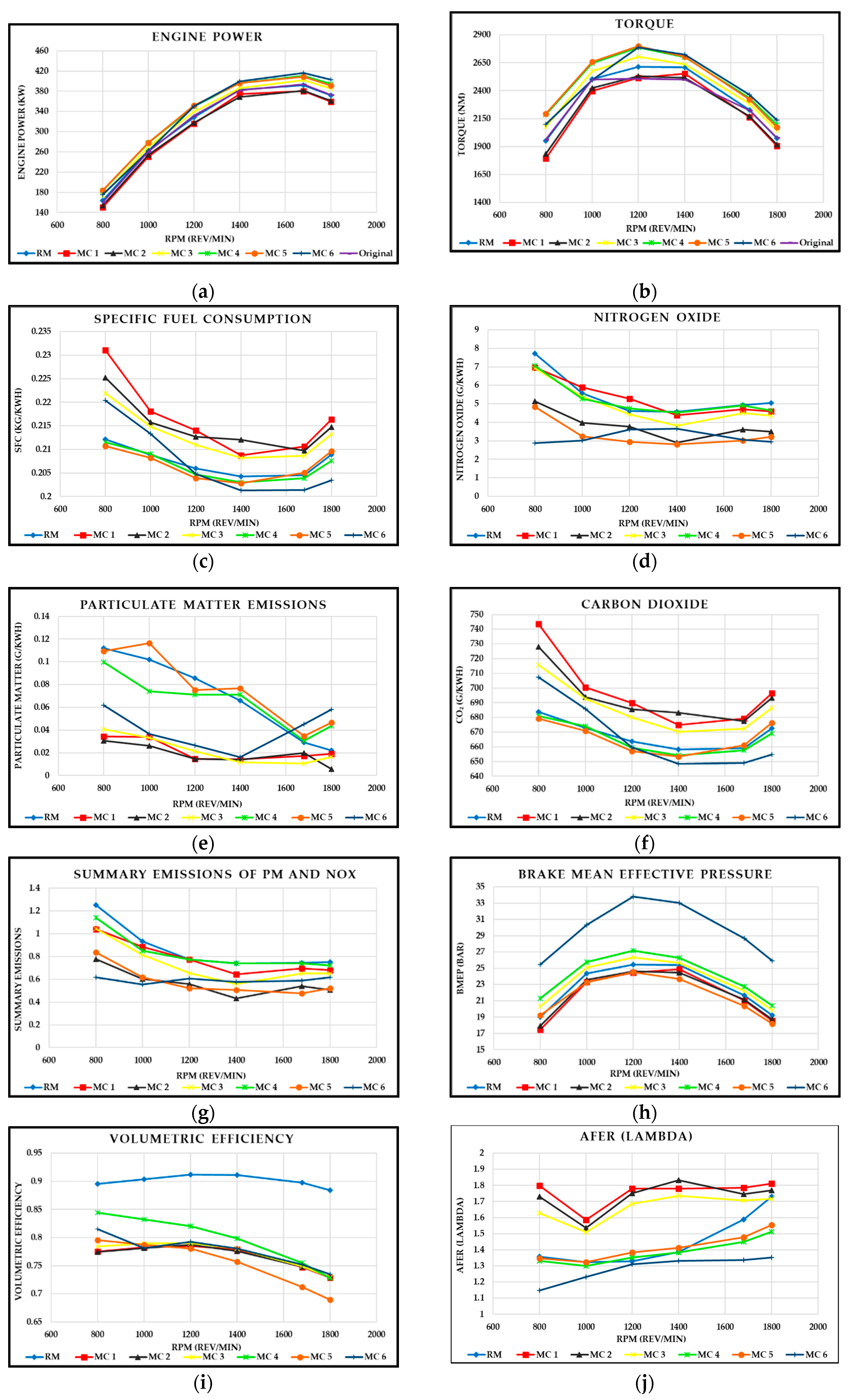
This study was conducted with the aim to achieve simultaneous improvement in heavy-duty engine performance and emission characteristics by applying Miller cycle to a conventional diesel engine with the use of conventional diesel fuel and biodiesel fuel blends. The analysis was based on the multi-parametric multi-stage optimization of engine design and operating parameters.

2. Materials and Methods

This section is split into two parts, the simulation of the CDE, accompanied by the creation of the reference model (RM) and the application of MC to the CDE accompanied by its optimization. These goals have been achieved through using the DIESEL-RK software. To achieve the best possible results, 1 model of CDE (RM) and 6 models of MC were created. Each model was made up of different parameters and engine design. The DIESEL-RK is a simulation software that represents full thermodynamic cycles. The software has the capability of simulating and optimizing the operation method of 2-stroke and 4-stroke internal combustion engines, including all the types of boosted engines. Another feature of the program is the simulation of the MC, as it can be applied to a CDE by changing some variables such as IVC degrees and PR_c [19,20,21]. The package also includes the following features which were used in this study:

• Analysis and optimization of combustion and emission.
• Analysis and optimization of EGR system.
• Matching and optimization of turbocharger and bypasses.
• Optimization of valve timing.
• Performance prediction of the engine power and torque curves.
• Prediction and optimization of fuel consumption.

2.1. Reference Model (RM) Setup

A research engine (390 kW) was the selected turbocharged HDDE with data available in our research group. We used the available experimental data of engine power and torque over rpm range, and also, the parameters of a real engine. The reference model was created to precisely match the power and torque of the real engine. All multiparametric analysis and improvements associated with Miller cycle were compared with the reference model. General parameters and specification for this engine are given in

Table 1. General parameters and specifications of the research diesel engine.

General Parameters and Specifications
Bore x Stroke	130 × 162 mm
Displacement	12.9 litres
Compression Ratio	18.5 to 1
Number of Cylinders	6 in-line
Number of Valves	4 valves per cylinder
Maximum Output	390 kW (530 hp) at 1680 RPM
Maximum Torque	2500 Nm at 1000–1425 RPM
Idling Mode	800 RPM
Fuel Type	Diesel, Biodiesel
Fuel Injection	Common rail with 2 high pressure pump units
Injection Pressure	Maximum 2500 bar
Turbocharger	Variable-Geometry Turbocharger
Emission Regulations	EURO-VI

.

2.1.1. Parameters Calculation

The following points refer to several parameters that were calculated for every regime. Notice that the fluctuations of cycle fuel mass values are expected in order to find the best combination.

2.1.2. Cycle Fuel Mass

$${\mathrm{m}}_{\mathrm{f}}=\frac{\mathrm{SFC}\ast \mathrm{Power}}{\mathrm{RPM}\ast \mathrm{icyl}\ast 30}$$

(1)

-

m_f = cycle fuel mass (grams);

-

SFC = specific fuel consumption, usually for HDDE ranges between 225–230 (g/kWh);

-

Power = engine power corresponding to the RPM;

-

icyl = number of cylinders (in this case, icyl = 6).

2.1.3. Start of Injection/Ignition Timing (SOI) (Degrees before TDC)

This parameter was calculated using the 1D scanning function for each regime separately. In this case, the SOI values for HDDE range between 3–14 degrees. Figure 1 shows the 1D scanning results. The selection criterion for every SOI is to match the minimum fuel consumption with the maximum performance, maximum pressure rise rate (dp/dTheta), values between 5–6 bar/deg, and maximum cylinder pressure, 180–200 bar. Regarding the maximum cylinder pressure, the values could be slightly higher according to the research reported in the literature [22].

2.1.4. Exhaust Gas Recirculation

EGR is 6% and corresponds to the research conventional heavy-duty engine, this is due to Euro-VI strict regulations for the emissions.

2.1.5. Turbocharger Efficiency (ηTC) and Compressor Adiabatic Efficiency (HP-stage) (ηC):

$$\eta \mathrm{C}=\sqrt{\eta \mathrm{TC}}$$

(2)

-

ηTC = approximately 0.49–0.51 for HDDE.

2.1.6. Inlet Pressure Losses (before Compressor) and Differential Pressure in Exhaust

At maximum engine power, the losses in the exhaust are about 0.04 bar while the inlet losses before the compressor are about 0.02 bar. At lower RPM, these values are slightly smaller.

2.1.7. Injection Pressure

The maximum injection pressure at the maximum engine power is 2300–2500 bar at maximum engine speed. Therefore, for the rest of the regimes, the injection pressure varied and was calculated by the following equation:

$${\mathrm{P}}_{\mathrm{inj}}={\mathrm{P}}_{\mathrm{inj}}\mathrm{p}\max \ast {\left(\frac{\mathrm{RPM}}{{\mathrm{RPM}}_{\mathrm{pmax}}}\right)}^{1.244}$$

(3)

-

P_{inj_pmax} = Maximum injection pressure at maximum power, 2300 bar;

-

RPM = Corresponding engine speed (800, 1000, 1200, 1400, 1680 and 1800);

-

RPM_pmax = 1680 RPM.

This equation was used to estimate the duration of the injection when the injection pressure of the fuel is registered. Additionally, this equation contributes to the prediction of the injection pressure for the rest of the regimes.

2.1.8. Compressor Pressure Ratio (PR_c)

The Compressor Pressure Ratio (PR_c) settings have been selected from the empirical correlation of PR_c against the break mean effective pressure (BMEP) that is imbedded in the DIESEL-RK program. This correlation and selection of PR_c that corresponds to BMEP 15–25 bar is shown in Figure 2.

2.2. Miller Cycle Diesel Engine Model Setup

For the application of the MC, the degree of IVC and the PR_c value needed a modification. Compared to the CDE that use 40 to 50 degrees after bottom dead center (ABDC), the MC have different values that range between 20 degrees and −20 degrees ABDC. That minus sign means that the intake valve closes 20 degrees before bottom dead center (BBDC). The function of 2D scanning was used to represent two arguments, the IVC on the y-axis, and the PR_c on the x-axis, while the isolines represent the AFER, NO, PM, and SFC results as functions of these two arguments. From this graph, it was feasible to observe which IVC degrees and PR_c would produce the most preferable values for AFER and the lowest values for NO, PM, and SFC. Figure 3 represents the IVC vs. PR_c at 1680 RPM, the point 0 is the BDC, the positive values correspond to the LIVC and the negative values to the EIVC. Therefore, the 10 degrees BBDC were selected for all the MC models, as the process of 2D scanning was conducted for all the engine speeds (800, 1000, 1200, 1400, 1680 and 1800 rpm) and showed the same trends. The reason behind the selection of 10 degrees BBDC is shown in Figure 3, emissions at reduced level occur at this point, whereas there is a compromise between the AFER and lower values of boost pressure. It was not desirable to have an AFER that would exceed 1.8 as it would result in the formation of very lean mixture which would lead to a possible reduction in engine efficiency. Additionally, SFC showed increasing trends as the IVC degrees were closer to the region of ABDC than when it was closer to the region of BBDC.

2.2.1. Optimization of Miller Cycle

It was observed that the outcome results needed optimization as the performance was poor compared to the RM. In this case, a multiparametric optimization was performed that considered all the variable factors and endeavors to match in order to find the best combination in relation to a goal function, independent variables and restrictions [21,23]:

2.2.2. Goal Function

Zj = Zj (Xk)

(4)

Through the goal function of the multiparametric optimization, several parameters of the efficiency can be included. Zj is the function of variables (i.e., SFC, Volumetric efficiency, BMEP and a complex of air pollutants (NOx + PM). Therefore, in this case, Zj = (NOx + PM), the goal function of this case is the minimization of the complex of air pollutants (NOx + PM) that is determined by the following equation:

$$\mathrm{SE}={\mathrm{c}}_{\mathrm{PM}}\frac{\mathrm{PM}}{{\mathrm{PM}}_0}+{\mathrm{C}}_{\mathrm{NO}}\frac{\mathrm{NOx}}{{\mathrm{NOx}}_0}$$

(5)

where:

-

C_PM = 0.5 and C_NO = 1.0. which are the values of emission weighting coefficients;

-

PM_o = 0.15 and NO_xo = 7 which are base values of pollutants;

-

PM and NOx - represent the values of emissions (g/kWh) at a specific engine speed.

The values of emission weighting coefficients C_PM, C_NO, PM_o, and NO_xo were defined through empirical correlations obtained by Diesel-RK developers by validating the program against the range of engine experiments.

2.2.3. Vector of Independent Variables

Xk_min < Xk < Xk_max

(6)

The vector of the independent variables Xk is defined by the design parameters of the engine. The independent variables are within the restricted solution area. The upper and lower limits can be set through the independent variable list.

• X₁ = Injection Timing deg. BTDC
• X₂ = HP stage PR_c
• X₃ = EGR

2.2.4. Restrictions

Y_i = Y_i (Xk)

(7)

The control of thermal and mechanical stresses and emission levels are crucial points during the search for optimum combination. These parameters can be set through the restriction table and contribute to the constraint of the limits in order to assist the software to find the optimal combination which can be seeking within a pool of data. A mathematical model combines the analytical relation among the goal function, restrictions, and the vector of independent variables. Consequently, the optimization of the engine constitutes a problem of non-linear programming where the function Zj is the optimum point that the software is looking for through the set limitations.

Therefore, the restrictions are defined by [19,24]:

Y_{i min} < Y_i < Y_{i max}

(8)

• Y₁ = AFER
• Y₂ = Engine Power
• Y₃ = SFC
• Y₄ = Volumetric Efficiency
• Y₅ = NOx emissions

The solution of optimization problems becomes more complicated due to the registration of specific restrictions; hence, the conditional optimization problem is reduced in relation to the non-conditional optimization problem with the result of the development of a better algorithm. In the optimization solution, the penalty method function accounts for the effective means of the restrictions. Essentially, this method contributes to the optimization process in the case where the restrictions are violated, and thus value is assigned to the minimum goal function. Therefore, the penalty value increases as the violated restrictions increase. The goal function F is derived by the sum of three members: C_zj, C_yi, C_xk

$$\mathrm{F}={\mathrm{C}}_{\mathrm{zj}}\ast {\overline{\mathrm{Z}}}_{\mathrm{j}}+{\displaystyle \sum }_{\mathrm{i}=1}^{\mathrm{n}}\left({\mathrm{C}}_{\mathrm{yi}}\ast \Delta {\overline{Y}}_i^2\right)+{\displaystyle \sum }_{\mathrm{k}=1}^{\mathrm{m}}\left({\mathrm{C}}_{\mathrm{xk}}\ast \Delta {\overline{X}}_k^2\right)$$

(9)

-

C_zj = (influence coefficient) of ICE relative parameter (SE);

$${\overline{\mathrm{Z}}}_{\mathrm{j}}=\frac{{\mathrm{Z}}_{\mathrm{j}}}{{\mathrm{Z}}_{\mathrm{jmean}}}$$

(10)

-

C_yi = penalty factor for values out of permitted area of Y_i;

-

Restrictions violation relative ($\Delta \overline{Y_i}$);

-

C_xk = penalty factor for values out of permitted Xk;

-

Independent variable k relative value of leaving the restricted area ($\Delta {\overline{X}}_k$).

$$\Delta {\overline{Y}}_i=\left\{\begin{array}{cc}\frac{Y_i-Y_{i \min } }{Y_{i mean}}& \hfill if\hspace{1em}\hspace{1em}\hspace{1em}\hspace{1em} Y_i<Y_{i \min }\\ 0& if\hspace{1em}\hspace{1em}{Y}_{i \min }\le Y_i\le Y_{i \max }\\ \frac{Y_i-Y_{i \text{max}} }{Y_{i mean}}& \hfill if\hspace{1em}\hspace{1em}\hspace{1em}\hspace{1em} Y_i>Y_{i \text{max}}\end{array}\right\}$$

(11)

$$\Delta {\overline{X}}_k=\left\{\begin{array}{cc}\frac{X_k-X_{k \min } }{X_{k mean}}& \hfill if\hspace{1em}\hspace{1em}\hspace{1em}\hspace{1em} X_k<X_{k \min }\\ 0& \hfill if\hspace{1em}\hspace{1em}{X}_{k \min }\le X_k\le X_{k \text{max}}\\ \frac{X_k-X_{k \text{max}} }{X_{k mean}}& \hfill if\hspace{1em}\hspace{1em}\hspace{1em}\hspace{1em} X_k>X_{k \text{max}}\end{array}\right\}$$

(12)

2.2.5. Protocol of Optimization

By completing the multiparametric optimization and running the analysis for every regime separately, a table with a protocol of optimization includes all the median and optimum results of the engine simulations. The optimization protocol specifies which independent variables should be changed in the operating mode in order to optimize the goal function taking into account specified restrictions. The suggested independent variable values generated through the multiparametric optimization replace the previous ones in the operating mode and therefore the analysis runs again to produce new improved results.

3. Results and Discussion

3.1. Engine Design and Operating Parameters

To achieve the objective of this study, some criteria were set to be met by the MC diesel engine. These criteria refer mainly to the enhanced performance of the engine, minimum exhaust emissions and the reduced SFC. Therefore, 6 models based on the operation of MC were created to produce data that can fulfil the criteria of the objective. Each model was made up of different engine operating and design parameters compared to the RM, while every change in those aspects were based on the multiparametric optimization.

Table 3. Engine design parameters for all models.

Design Parameters	RM	MC 1	MC 2	MC 3	MC 4	MC 5	MC 6
Compression Ratio	18.5	18.5	18.5	18.5	18.5	22	18.5
Bore (mm)	130	130	130	130	130	130	130
Stroke (mm)	162	162	162	162	162	180	130
Displacement (l)	12.9	12.9	12.9	12.9	12.9	14.3	10.3
Nº of Nozzle holes	7	7	7	7	8	8	10
Nozzles Bore (mm)	0.222	0.222	0.222	0.222	0.222	0.222	0.222
IVC (Degrees)	46 ABDC	10 BBDC	10 BBDC	10 BBDC	10 BBDC	10 BBDC	10 BBDC

and

Table 4. Engine operating parameters for all models.

	Parameters Per rpm	800	1000	1200	1400	1680	1800
RM	Cycle fuel mass (g)	0.241	0.304	0.313	0.31	0.265	0.24
	SOI [Degrees BTDC]	3.75	5	6	7.25	8.5	8.75
	PRc	2.5	3.15	3.25	3.4	3.5	3.55
	EGR	0.06	0.06	0.06	0.06	0.06	0.06
MC 1	Cycle fuel mass (g)	0.241	0.304	0.313	0.31	0.265	0.24
	SOI [Degrees BTDC]	3.75	5	6	7.25	8.5	8.75
	PRc	4	4.5	5.25	5.25	4.75	4.5
	EGR	0.06	0.06	0.06	0.06	0.06	0.06
MC 2	Cycle Mass fuel (g)	0.241	0.304	0.313	0.31	0.265	0.24
	SOI [Degrees BTDC]	2.5	3.5	4.5	5.75	7	7.25
	PRc	3.9	4.4	5.15	5.45	4.65	4.4
	EGR	0.076	0.076	0.064	0.064	0.064	0.064
MC 3	Cycle Mass fuel (g)	0.269	0.322	0.332	0.319	0.277	0.253
	SOI [Degrees BTDC]	3.75	5	6	7.25	8.5	8.75
	PRc	4	4.5	5.25	5.25	4.75	4.5
	EGR	0.06	0.06	0.06	0.06	0.06	0.06
MC 4	Cycle Mass fuel (g)	0.269	0.322	0.332	0.319	0.277	0.253
	SOI [Degrees BTDC]	2.5	3.5	4.5	5.75	8.5	9
	PRc	2.95	3.6	3.95	4	3.95	3.95
	EGR	0.06	0.06	0.06	0.06	0.065	0.07
MC 5	Cycle Mass fuel (g)	0.269	0.322	0.332	0.319	0.277	0.253
	SOI [Degrees BTDC]	3	3	4.5	5.75	7.25	8
	PRc	2.95	3.6	3.95	4	3.95	3.95
	EGR	0.1	0.1	0.1	0.1	0.1	0.1
MC 6	Cycle Mass fuel (g)	0.269	0.31	0.332	0.319	0.277	0.253
	SOI [Degrees BTDC]	1	2.5	3.75	5.5	6.5	7
	PRc	3.5	4.65	5.25	5.2	4.75	4.5
	EGR	0.12	0.12	0.12	0.12	0.12	0.12

show the design and operating parameters of the original engine that were used to create the RM and MC models.

3.1.1. Miller Cycle Model 1

The MC 1 was the first model created when the data was emerged from the 2D scanning function of the RM. The basic rationale on why this function was used is that the user can be informed when a certain value of IVC and compressor PR_c is selected for the engine at a certain engine speed; after running the software, the following outcomes NOx, PM, SFC, and AFER would produce the corresponding values that the 2D scanning graphs illustrate. Additionally, this function informs the user which values of IVC and PR_c would produce the least NOx, PM and SFC. As stated in Section 2.2, 10 degrees BBDC was the selected value for the IVC for all the engine speeds of MC models, as it was observed that this value could produce less emissions, whilst the PR_c values varied at each engine speed, as can be seen in Table 4. The Zeldovich mechanism was used to simulate the formation of NOx for all the models.

The findings of MC 1 simulation were compared to the RM in Section 3.2 and show that the performance of the engine was affected by the change in the IVC degrees and reduced by 4.1%. The reason behind these results is due to the fact that by changing the degrees of the IVC, the volumetric efficiency dropped to a great extent, as shown in Figure 4i. More specifically, the volumetric efficiency of the RM ranges between 88.3–91.1%, whilst for the MC 1 it ranges between 72.8–78.5%. For the MC 1, there is a drop that fluctuates between 9.8–18.3%. Even with the increased boost pressure, it could not help improving the performance of the engine. Furthermore, NOx, NO and PM decreased by 22%, 1.3% and 58.8%, respectively. This reduction in emissions is basically due to the decreased temperature within the chamber during the combustion, as shown in Figure 4m, and the better combustion of the mixture due to the increase in the AFER, as shown in Figure 4j. The greater AFER led to an increase in SFC by 4.3%, subsequently the same occurred for CO₂, as shown in Table 6a.

3.1.2. Miller Cycle Model 2

The MC 2 was reproduced from the MC 1, where MC 2 had the same results for PR_c and degrees of IVC as MC 1 from 2D scanning. However, the MC 2 was subjected to a multiparametric optimization with a goal on the further reduction of emissions. The operating parameters shown in Table 4 are the results that emerged from the multiparametric optimization. Below, there are variable factors set manually to run the multiparametric optimization.

Goal function (Equation (5)—Section 2.2):

-

$\mathrm{SE}={\mathrm{c}}_{\mathrm{PM}}\frac{\mathrm{PM}}{{\mathrm{PM}}_0}+{\mathrm{C}}_{\mathrm{NO}}\frac{\mathrm{NOx}}{{\mathrm{NOx}}_0}$

Independent variables:

-

Injection Timing: 2.5–12 degrees BTDC

-

HP stage PR_c: 2–7

-

EGR: 5–30%

Restrictions:

-

AFER: 1.3–2.2

-

Engine Power (Varied for every engine speed)

-

SFC: 0.18–0.3 kg/kWh

-

Volumetric Efficiency: 0.65–1

-

NOx emissions: 0–8.5 g/kWh

Table 3 and Table 4 represent the final design and operating parameters of the MC 2 emerged after the multiparametric optimization. The multiparametric optimization process produced many scenarios in which each one was unique and included suggested combinations of independent variable values that could help to achieve the goal function. The new values were registered manually in the operating mode. In relation to MC 1 findings, the MC 2 shows that it achieved better results compared to the RM, as shown in Table 6b.

Both engine power and torque decreased by 3.6%, whilst exhaust gas emissions NOx, NO, PM decreased by 42.7%, 29.1% and 69% respectively. The performance of the engine for this model appears to be better than MC 1 and closer to that of RM. Additionally, the emissions seem to have fallen even further compared to those of RM; however, SFC and CO₂ increased by 3.66% and 3.8%, respectively. These results may look better in relation to the MC 1 but comparing them to the RM they are not so good for economic and environmental implications. As it can be seen, the MC 2 has the same trends for performance, emissions, and SFC as those of MC 1. However, the results were still not satisfactory to meet the objectives of this study as they showed lower performance and increase in SFC in comparison to those of RM.

3.1.3. Miller Cycle Model 3

The MC 3 was developed based on the MC 1 like all the other models, but since models 1 and 2 appeared to have a reduced performance relative to that of RM, it was opted to increase manually the cycle fuel mass in order to compensate the lack of performance. Thus, the following equation was used:

Cycle Fuel Mass:

$${\mathrm{Required}\mathrm{m}}_{\mathrm{f}}={\mathrm{Current}\mathrm{m}}_{\mathrm{f}}\ast \frac{\mathrm{Required}\mathrm{Power}}{\mathrm{Current}\mathrm{Power}}$$

(13)

By taking each engine speed separately, it was feasible to manually change the cycle fuel mass and run at different engine speeds to observe the change in engine power. Hence, what had occurred was the increase in the cycle fuel mass at each engine speed, while this resulted in enhanced engine power by an average of 10% in comparison to that of RM. However, a simultaneous increase in exhaust emissions was observed; thus, the model had to undergo a multiparametric optimization in order to reduce these emissions and simultaneously maintain the engine power. Consequently, in the process of multiparametric optimization, the requirements had increased for efficiently searching for protocols of optimization that would provide a better performance, reduced exhaust gas emissions and lower SFC in relation to the RM. The values in Table 4 have not been subjected to a significant change in relation to the MC 1 and 2. However, by comparing them to the RM, it was observed that the PR_c had risen 1–2 at each engine speed. Table 6c represents the performance, emissions and SFC outcomes emerged from the simulation of MC 3 in comparison to the RM results. Moreover, as it is observed from the percentage results shown in Table 6c, both the engine power and torque of MC 3 increased by 3.3% compared to those of RM. This improvement was due to the balanced combustion temperature and AFER; meanwhile, emissions of NOx, NO and PM decreased by 23.7%, 9.3% and 62.9%, respectively. The changes in the engine operating and design parameters might have had a good impact on the performance and emissions but in contrast it had a negative impact on the SFC and CO₂, which increased by 2.67% and 2.7%, respectively. Although the SFC of the MC 3 was observed to be lower than that of RM prior to multiparametric optimization, the optimization still could not make any improvement.

3.1.4. Miller Cycle Model 4

Reflecting onto the MC 3 results regarding some significant impacts on both SFC and CO₂, it was considered that these two outcomes were needed more optimization; thus, the MC 4 was prepared based on the MC 3 in order to develop a better model. It was decided to follow a different strategy, which included the increased number of nozzle holes from 7 to 8. However, this implementation had a direct impact on the injection pressure and duration as it was reduced to a very large extent, and therefore, both of these parameters had to be readjusted to the previous values using Equation (3). Following the multiparametric optimization process with the same limitations of goal function, independent variables, and restrictions such as those for MC 2, the process suggested some input values that were later applied to the MC 4. Table 3 shows the change in the number of nozzle holes in comparison with other models subjected to the multiparametric optimization. The protocol of optimization suggested a reduction in the PR_c that varied between 1.05 to 1.20 at some individual engine speeds, as can be seen in Table 4 compared to the other models. At the same time, SOI and some EGR values had to be changed and replaced with values that could deliver better results. The cycle fuel mass remained the same as that for MC 3, but, in comparison with the RM, there was a slight change in these values.

For the first time in this study, the SFC and CO₂ outcomes appeared to be lower than those of RM, as a matter of fact, both of them were reduced by 0.39% and 0.40% respectively, as shown in Table 6d. Additionally, the performance of both the engine power and torque increased to 6.5%, and this amount corresponded to the highest increase in performance in this study. It is worth mentioning that while increasing the number of nozzle holes and decreasing the PR_c, the volumetric efficiency was also improved in relation to that of other MC models. The volumetric efficiency of the MC 4 ranged between 72.8% and 84.4%. These values represent a reduction of 3.9%-13.8% in comparison to that of RM. Even though the performance, SFC and CO₂ looked promising, unfortunately NOx and PM were proven to decrease the quality of this model, as both of them were increased by 0.4% and 3.5%, respectively, compared to those of RM.

3.1.5. Miller Cycle Model 5

Including the different changes in operating and engine design parameters so far, no results have been found that could be promising to fulfil the objective of this study. During the simulations with other models, it was observed that increased SFC resulted in reduced exhaust emissions and that CO₂ always follows the SFC trend. The displacement of MC 5 was increased intentionally compared to that of MC 4 in order to increase fuel consumption as it was lower than that for RM, anticipating that the emissions will be reduced, and, finally, all the results will come to a balance as the objective of this study. Thus, for the MC 5 (Table 3), it was decided to increase both the piston’s stroke from 162 to 180 mm and CR from 18.5 to 22, with an expectation that these two new adjustments would improve the overall performance of the MC diesel engine. The original bore/stroke ratio of the RM was 0.80, described as an undersquare (long stroke), while the redesigned bore/stroke ratio changed to 0.72 for the MC 5. Furthermore, for the more efficient reduction of the emissions, the increase in EGR was deemed necessary and therefore the value had risen to 10%, whilst the PR_c value remained the same as that of MC 4. Another change that was made in MC 4 was the SOI degrees because, after some model simulations, various problems related to the maximum rate of pressure rise and SFC appeared. The 1D scanning function was used in this case to correct the SOI degrees in order to develop a better outcome for MC 5.

The results of the simulation for MC 5 did not have a major impact on the performance in relation to MC 4, as engine power and torque decreased only by 0.1% and maintained an increment of 6.4% compared to the RM, as shown in Table 6e. However, NOx and NO emissions were reduced by 35.6% and 38.1%, respectively. SFC and CO₂ remained 0.34% and 0.30% lower than those of RM. The only issue with this model was the PM emissions, which increased to 24.7% compared to those of RM.

3.1.6. Miller Cycle Model 6

The target for this model was to reduce the piston stroke from 162 to 130 mm to create a squared bore/stroke ratio, so both bore and stroke had dimensions of 130 mm. The reason for changing the stroke dimensions was due to the fact that, by reducing the displacement of the engine, the SFC is reduced and the emissions will be reduced. MC 6 has an increased number of nozzle holes from 8 to 10 for the purpose of achieving the complete combustion of the mixture in the cylinder. The ratio of the EGR was increased manually to reduce the emissions but expecting that this would have a negative impact on the engine performance. The multiparametric optimization function was used, but this time it had a goal to further optimize the SFC. Another useful function that was applied to MC 6 was the 1D scanning to readjust the SOI to improve the performance. Table 3 and Table 4 show the engine final design and operating parameters for MC 6. The values for PR_c ranged between 3.5 and 5.25. As shown in Table 6f, engine power and torque represent the performance of the engine that was improved by 5.5% compared to that of RM. NOx, NO, PM and CO₂ emission were reduced by 30.2%, 38.2%, 5.5% and 0.1%, respectively, and both SFC and CO₂ showed negligible change. These results show that MC 6 was turned to be the best model in respect to exhaust gas emissions. Overall, MC 6 can be considered to be the most promising model among all the MC models for this study and it is the only model that meets all the criteria of the set objectives, which is to achieve the better engine performance, lower emissions and reduced fuel consumption.

3.2. Summary Results for All the Models

The following figures refer to the performance of RM and all six MC models. They show the comparison of all the models for the engine performance, exhaust gas emissions and fuel consumption.

Table 5. Important outcomes of RM per engine speed.

RM-Outcome	Engine Speed—RPM (rev/min)
	800	1000	1200	1400	1680	1800
Engine Power (kW)	163.57	262.09	328.34	382.52	391.76	372.25
Torque (Nm)	1952.6	2502.9	2613	2609.3	2226.9	1975
SFC (kg/kWh)	0.21217	0.20879	0.20591	0.20423	0.20456	0.20889
NOx (ppm)	1730.5	1301.6	1087.5	1041.4	982.86	906.22
NO (g/kWh)	7.7256	5.5837	4.6163	4.5633	4.9259	5.047
PM (g/kWh)	0.11214	0.10179	0.085621	0.065817	0.029258	0.021912
CO₂ (g/kWh)	683.75	672.99	663.59	658.22	659.02	672.7

refers to the outcomes of the RM at different engine speeds, whereas all models will be compared to, in contrast to all the other results that emerged from the simulation of six MC models.

Table 6. Engine performance operating on Miller Cycle in comparison to RM.

(a)
Outcome	MC 1 RPM						Average Increase/Decrease
	800	1000	1200	1400	1680	1800
Power (kW)	−8%	−4%	−4%	−2%	−3%	−3%	−4.1%
Torque (Nm)	−8%	−4%	−4%	−2%	−3%	−3%	−4.1%
SFC (kg/kWh)	9%	4%	4%	2%	3%	4%	4.3%
NOx (ppm)	−38%	−17%	−15%	−27%	−18%	−16%	−22.0%
NO (g/kWh)	−10%	5%	14%	−4%	−5%	−9%	−1.3%
PM (g/kWh)	−69%	−67%	−83%	−78%	−41%	−14%	−58.8%
CO₂ (g/kWh)	9%	4%	4%	3%	3%	4%	4.3%
(b)
Outcome	MC 2 RPM						Average Increase/Decrease
	800	1000	1200	1400	1680	1800
Power (kW)	−6%	−3%	−3%	−4%	−3%	−3%	−3.6%
Torque (Nm)	−6%	−3%	−3%	−4%	−3%	−3%	−3.6%
SFC (kg/kWh)	6%	3%	3%	4%	3%	3%	3.66%
NOx (ppm)	−51%	−41%	−40%	−54%	−36%	−35%	−42.7%
NO (g/kWh)	−33%	−29%	−18%	−36%	−27%	−31%	−29.1%
PM (g/kWh)	−73%	−74%	−83%	−79%	−32%	−73%	−69.0%
CO₂ (g/kWh)	6%	3%	3%	4%	3%	3%	3.8%
(c)
Outcome	MC 3 RPM						Average Increase/Decrease
	800	1000	1200	1400	1680	1800
Power (kW)	6%	3%	3%	1%	3%	3%	3.3%
Torque (Nm)	6%	3%	3%	1%	3%	3%	3.3%
SFC (kg/kWh)	5%	3%	2%	2%	2%	2%	2.67%
NOx (ppm)	−30%	−19%	−27%	−35%	−18%	−14%	−23.7%
NO (g/kWh)	−10%	−3%	−4%	−16%	−8%	−13%	−9.3%
PM (g/kWh)	−64%	−67%	−75%	−82%	−64%	−25%	−62.9%
CO₂ (g/kWh)	5%	3%	3%	2%	2%	2%	2.7%
(d)
Outcome	MC 4 RPM						Average Increase/Decrease
	800	1000	1200	1400	1680	1800
Power (kW)	12%	6%	7%	4%	5%	6%	6.5%
Torque (Nm)	12%	6%	7%	4%	5%	6%	6.5%
SFC (kg/kWh)	0%	0%	−1%	−1%	0%	−1%	−0.39%
NOx (ppm)	−7%	−5%	2%	−1%	9%	4%	0.4%
NO (g/kWh)	−9%	−6%	3%	−1%	0%	−8%	−3.5%
PM (g/kWh)	−11%	−27%	−17%	8%	5%	98%	9.4%
CO₂ (g/kWh)	0%	0%	−1%	−1%	0%	−1%	−0.4%
(e)
Outcome	MC 5 RPM						Average Increase/Decrease
	800	1000	1200	1400	1680	1800
Power (kW)	12%	6%	7%	4%	4%	5%	6.4%
Torque (Nm)	12%	6%	7%	4%	4%	5%	6.4%
SFC (kg/kWh)	−1%	0%	−1%	−1%	0%	0%	−0.34%
NOx (ppm)	−36%	−41%	−37%	−38%	−34%	−29%	−35.6%
NO (g/kWh)	−37%	−42%	−36%	−38%	−39%	−36%	−38.1%
PM (g/kWh)	−2%	14%	−12%	17%	19%	113%	24.7%
CO₂ (g/kWh)	−1%	0%	−1%	−1%	0%	1%	−0.3%
(f)
Outcome	MC 6 RPM						Average Increase/Decrease
	800	1000	1200	1400	1680	1800
Power (kW)	7%	0%	7%	4%	6%	8%	5.5%
Torque (Nm)	7%	0%	7%	4%	6%	8%	5.5%
SFC (kg/kWh)	4%	2%	−1%	−1%	−2%	−3%	Negligible change over rpm range
NOx (ppm)	−59%	−40%	−21%	−14%	−25%	−23%	−30.2%
NO (g/kWh)	−63%	−46%	−22%	−20%	−38%	−41%	−38.2%
PM (g/kWh)	−45%	−64%	−69%	−76%	55%	166%	−5.5%
CO₂ (g/kWh)	3%	2%	−1%	−1%	−2%	−3%	-Negligible change over rpm range

a–f includes a percentage of an increased/decreased outcomes per engine speed compared to RM. Additionally, the last column of each table represents an average value (either increased or decreased) that was calculated based on the related final outcomes. As can be seen in Table 6a, for the engine speeds 800, 1400, 1680 and 1800 RPM, there is a reduction in NO emissions despite the increase in these emissions at 1000 and 1200 RPM, where the average result proves that an overall reduction in NO emissions can be achieved in comparison to the RM. It is worth mentioning that each model is a gradual optimization of the previous model, i.e., MC 6 model is built based on MC 5 model, MC 5 is based on MC 4, etc. Therefore, the best model was developed after a careful analysis and judgement of all six models, with a main factor on the outcome being the column of an average increase/decrease. The green colour represents the achievement of the goal, and the red colour represents the non-achievement of the goal. The model MC 6 with all green values is the best model for this study.

3.3. Comparison of Engine Performance, SFC and Emissions

Figure 5a below represents the difference between engine power and SFC of RM and MC 6 at different RPMs. The engine power for RM, which is illustrated by a light blue colour, varies within 163–392 kW, with its peak power of 392 kW occurring at 1680 RPM. Engine power for MC 6 model is represented by a yellow colour and ranges between 175–416 kW with the peak power occurring at 1680 RPM. SFC of RM is shown by a red colour and fluctuates between 0.2042–0.2121 kg/kWh, with the least fuel being consumed at 1400 RPM. The SFC of MC 6 is shown by a black colour and ranges between 0.2013 and 0.2203 kg/kWh but this time the least fuel is consumed at 1680 RPM. For the RM and MC 6, the gap between the engine power and SFC is illustrated by orange and green colours, respectively. What has been achieved through the MC 6 simulation and optimization is an extended mapping between the engine power and SFC at the range of working RPMs that heavy-duty engines usually operate. That means the MC 6 consumes 0.2013 kg/kWh fuel and produces 416 kW, which is the maximum engine power that occurs at 1680 RPM, unlike the RM that consumes 0.2045 kg/kWh fuel and produces 392 kW at the same engine speed. At 1400 RPM, the RM and MC 6 consume 0.2042 kg/kWh and 0.2013 kg/kWh fuel and produce 382 and 399 kW, respectively. Therefore, MC 6 consumes less fuel for more power compared to the RM, which needs more fuel for less power.

Figure 5b shows the same conditions as those in Figure 5a, but, in this case, it compares the torque with SFC instead of engine power. The torque of the MC 6 seems to be improved equally at two different engine speeds compared to the RM. More specifically, the torque of the MC 6 is 2787 Nm and 2724 Nm at 1200 RPM and 1400 RPM and consumes 0.2047 kg/kWh and 0.2013 kg/kWh of fuel, respectively. The torque of the RM is 2613 Nm at 1400 RPM and consumes 0.2042 kg/kWh of fuel. Therefore, MC 6 consumes less fuel for more torque compared to RM, whilst the RM needs more fuel to consume in order to produce maximum torque and even in this case, it cannot reach the torque levels of the MC 6.

Trucks tend to operate at engine speeds ranging between 1200 and 1800 RPM and, for this reason, it is important that, at these engine speeds, the fuel consumption is at the lowest possible point. Trucks circulate mainly in highways across the country and not in city centers that are full of traffic lights and congestion making them stop and start all the time. Engine speeds at 600–800 RPM are mainly needed to accelerate the truck from a zero speed to a certain level of driving speed; therefore, such speeds are less important in relation to the amount of fuel they burn. Unlike engine power that is more useful on straight highways, torque is more useful for uphill driving and especially when the truck is loaded. Figure 5 shows that the greater engine power occurs at speeds of 1400–1800 RPM, whilst torque is greater at lower engine speeds, such as 1000–1400 RPM.

The MC 6 was the only model that achieved a reduction in all emissions gases such as NOx, NO, PM, and CO₂ compared to those of RM. The summary of emissions (SE) of NOx and PM, as shown in Figure 6a, was calculated using the Equation (5) mentioned in Section 2.2. This equation was used in the optimization goal function. It is worth mentioning that CO₂ emissions had the same trend as that of SFC in all models.

By observing Figure 6a, it can be noticed that a mapped gap had been established between the summary of emissions of RM and MC 6 at engine speeds ranging between 800 and 1200 RPM. This is a great reduction benefit considering that these engine speeds are mostly used in city roads that can cause congestion and long queues of traffic. The AFER of the MC 6 ranges from 1.14 to 1.35, while RM’s ratio ranges at 1.35–1.75, as shown in Figure 6b. The air–fuel mixture of the MC 6 is richer than that of RM because MC 6 has a twice higher EGR rate, and due to higher EGR rate, combustion temperature is reduced that helps the reduction of NOx emissions, as shown in Figure 4d. Therefore, cumulative Summary of Emissions decreases for MC6 model.

3.4. Mechanical and Indicated Efficiency

The mechanical efficiency depends on the indicated efficiency of the engine. Indicated thermal efficiency is defined as the ratio of the work produced per cycle to the amount of fuel energy supplied per cycle that can be released in the combustion process. Mechanical efficiency is defined as a parameter that shows how the useful work produced through combustion is transferred into the engine output; it is the ratio of the brake thermal efficiency over an indicated thermal efficiency. With the increase in engine rpm, friction power increases. Friction power is defined as the power required to overcome the flow friction, friction of the bearings, pistons, and other mechanical components of the engine, and to drive the engine accessories. Therefore, although with the increase in engine speed the indicator efficiency has tendency to increase, the mechanical efficiency decreases as a result of losing the energy due to friction. The relation between mechanical and indicated thermal efficiency is shown in the equations below.

Indicated thermal efficiency:

$${\eta }_{it}=\frac{P_i}{\dot{m_f} · fuel calorific value \left[\frac{kJ}{kg}\right]}$$

(14)

Break thermal efficiency:

$${\eta }_{bt}=\frac{P_b}{\dot{m_{f }}· fuel calorific value \left[\frac{kJ}{kg}\right]}$$

(15)

Mechanical efficiency:

$${\eta }_m=\frac{{\eta }_{bt}}{{\eta }_{it}}$$

(16)

where P_i is indicated power, P_b is break power, and $\dot{m_{f }}\mathrm{is}\mathrm{the}\mathrm{fuel}\mathrm{mass}\mathrm{flow}\mathrm{rate} \left(\frac{kg}{sec}\right)$

By comparing Figure 7, it was observed that a lower indicated efficiency led to a greater mechanical efficiency, while, on the other hand, a lower mechanical efficiency led to a greater indicated efficiency, and this applies for all the models without exception. Regarding all the MC models, the MC 6 has the greater mechanical efficiency that ranges between 90.53–92.57% for all engine speeds, and that gives an average of 91.68% efficiency. However, at the same time, this model has the lowest indicated efficiency that ranges between 41.61% and 46.65% with an average of 44.94%. On the other hand, the RM’s indicated efficiency and mechanical efficiency average values are 47.08% and 90.42%, respectively. This concludes that the MC 6 model can offer a greater mechanical efficiency, but lower indicated efficiency compared to the RM. One of the main features of the MC that succeeds when applied to a diesel engine is the improved thermal efficiency as mentioned in the introduction section. Through this study, it was possible to prove this fact, and, more specifically, the models MC 1–5 had better thermal efficiency than that of RM, but at the same time these models had reduced mechanical efficiency.

3.5. Current Limitations and Challenges

High Pressure and Temperature within the Cylinder

Figure 4 m, n shows that the MC 6 has the higher in-cylinder temperature and pressure compared to those of all other MC models and RM model. This is due to the reduced displacement of the cylinder compared to that of other models. The displacement of the RM was 12.9 L, whilst for MC 6, the new displacement was 10.3 L, which means a 2.6-L downsizing of the engine. During the compression stroke, the air–fuel mixture within the chamber was at higher pressure due to the higher compression ratio in relation to the other models. This fact led to the greater combustion temperature and, as a result, the greater expansion stroke compared to the RM. Despite the reduced displacement, the MC 6 improved the performance of the engine and achieved lower emissions and SFC. The main issue is whether the cylinder block could endure this high boost pressure. The limitation imposed on the maximum pressure is due to the material that the cylinder block and head are made of. Usually, these two components are made of cast iron or aluminum alloys according to Myagkov L.L et al. [25]. According to Eilts P. et al. [22], the maximum in-cylinder pressure ranges between 180–200 bar, and in some cases, these numbers might be slightly higher. Figure 8 shows the cylinder maximum pressure for the MC 6 that ranges between 230–313 bar as these high-pressure values emerged from the high PR_c values shown in

Table 7. Boost pressure required from the turbocharger to produce the PR_c that the MC 6 diesel engine requires to deliver the outcomes stated in this study.

RPM	PRc	Ambient Pressure (bar)	Inlet Pressure Losses (bar)	Boost Pressure (bar)
800	3.5	1	0.005	3.48
1000	4.65	1	0.005	4.63
1200	5.25	1	0.005	5.22
1400	5.2	1	0.005	5.18
1680	4.75	1	0.02	4.65
1800	4.5	1	0.02	4.41

. These values are almost 115 bar higher than the maximum feasible pressure that a cylinder can withstand. Therefore, this is one factor that must be taken into consideration while manufacturing this new MC diesel engine. To endure high in-cylinder pressure levels for MC 6 new carbon-reinforced composites and alloys should be used. Another issue emerging during the simulation of the MC models is whether a type of turbocharger does exist which can produce up to 5.22 bar boost pressure, as shown in Table 7 and if it could be fit on an HDDE.

$$Boost Pressure Before Intercooler=\mathrm{PRc}\times \left(\mathrm{Ambient}\mathrm{Pressure}-\mathrm{Inlet}\mathrm{Pressure}\mathrm{Losses}\right)$$

(17)

As many studies suggest, the temperature drops with the application of the Miller cycle in a diesel engine. The same trend was observed in this study for models MC 1–5. Nevertheless, for MC 6, there was an increase in temperature compared to the RM. This increase in temperature is accompanied by the increased in-cylinder pressure; this is the link between the thermal and mechanical efficiency. The in-cylinder temperature for MC 6 ranges between 2052 and 2136 K and it is 66–204 K higher than that of RM. Another question that arises from this data is whether the materials that the engine is made of can withstand these high temperatures.

3.6. Analysis of Miller Cycle Model 6 with Biodiesel Fuel

Another component of this study was the application and simulation of engine performance and emissions with the use of biodiesel fuel. In this case, three types of biodiesel blends were applied to the MC 6 model with an aim of creating data that could be compared to the RM. These three types of blends consist of Soybean Methyl Ester (SME) B100%, B40%, and B20%. Figure 9 shows the outcomes of the engine performance for RM and MC 6 with three types of biodiesel blend.

Our results show the consistent trend for NOx emissions when in general NOx emission increases as biodiesel concentration in the blend increases. If we compare the results in

Table 8. Outcomes of the engine operating on three different types of biodiesel blends applied to MC model 6.

(a)
SME B-100% Outcome	Engine Speed—RPM (rev/min)						Average Increase/Decrease
	800	1000	1200	1400	1680	1800
Power (kW)	−10%	−18%	−13%	−14%	−13%	−12%	−13%
Torque (Nm)	−10%	−18%	−13%	−14%	−13%	−12%	−13%
SFC (kg/kWh)	24%	25%	21%	20%	20%	19%	21%
NO (g/kWh)	−21%	−8%	7%	10%	−9%	−19%	−7%
PM (g/kWh)	−76%	−85%	−90%	−89%	−55%	−19%	−69%
CO₂ (g/kWh)	10%	11%	8%	6%	6%	6%	8%
(b)
SME B−40% Outcome	Engine Speed—RPM (rev/min)						Average Increase/Decrease
	800	1000	1200	1400	1680	1800
Power (kW)	1%	−8%	−1%	−3%	−1%	1%	−2%
Torque (Nm)	1%	−8%	−1%	−3%	−1%	1%	−2%
SFC (kg/kWh)	10%	10%	7%	6%	6%	5%	7%
NO (g/kWh)	−35%	−23%	10%	13%	−7%	−19%	−10%
PM (g/kWh)	−59%	−69%	−76%	−89%	1%	102%	−32%
CO2 (g/kWh)	5%	4%	2%	1%	1%	0%	2%
(c)
SME B-20% Outcome	Engine Speed—RPM (rev/min)						Average Increase/Decrease
	800	1000	1200	1400	1680	1800
Power (kW)	5%	−4%	3%	1%	3%	4%	2%
Torque (Nm)	5%	−4%	3%	1%	3%	4%	2%
SFC (kg/kWh)	7%	7%	3%	2%	2%	1%	3%
NO (g/kWh)	−46%	−35%	−3%	−1%	−19%	−26%	−22%
PM (g/kWh)	−53%	−65%	−73%	−83%	26%	135%	−19%
CO2 (g/kWh)	4%	4%	1%	0%	−1%	−1%	1%

, it is seen that the lower the SME concentration in the blend, the higher NOx reduction, which is consistent with the trends obtained by many researchers. However, we must emphasize that this decrease is the average over the range of engine rpms as NOx formation varies at different engine operating regimes. As shown in Table 8, in fact, for most of the regimes at 1200 rpm (Max Torque) NOx increases compared to that of RM model and only for SME 20% we can see the NOx decrease at Max Torque regime.

Comparing the results in Table 8a–c, the best outcomes were produced with SME B20%. The results have shown some promising data as the performance (power and torque) of the engine increased by 2%, NO emissions reduced by 22%. Moreover, the higher content of oxygen in biodiesel compared to that of diesel fuel has contributed to the reduction of PM by 19%. On the other hand, the SFC and CO₂ have increased by 3% and 1%, respectively.

Despite the lower level of engine performance and increased SFC, compared to those of the MC 6 diesel model, the models with all three types of biodiesel blends (SME B100%, B40% and B20%) have shown that they have common positive outcomes, as for all three of them NO and PM emissions were reduced. More specifically, the model with SME B100% has proven a reduction of NO and PM by 7% and 69%, respectively, whilst the model with SME B40% has reduced NO and PM emissions by 10% and 32%, respectively. All three models with biodiesel blends have higher maximum in-cylinder pressure than that of RM, as shown in Figure 9j, while models with SME B40% and SME B20% have a higher maximum in-cylinder temperature. However, none of the three models with biodiesel blends have shown an improved indicated efficiency than that of RM, but those with SME B40% and SME B20% have achieved a better mechanical efficiency compared to that of RM.

4. Conclusions

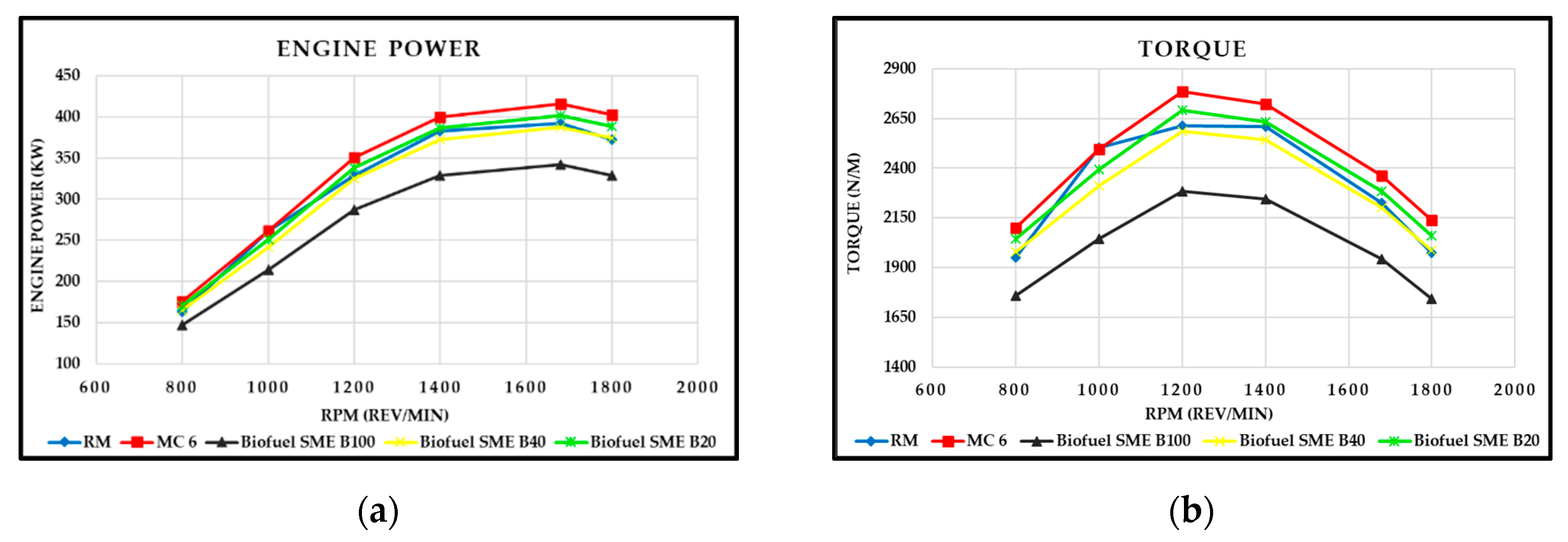
Reflecting on the extensive study of the application of the Miller cycle to a diesel engine, it has been found that at certain provided conditions the exhaust gas emissions can be substantially reduced. It was found that only a change in the degrees of IVC and an increase in PR_c were not sufficient to meet the criteria of the simultaneous improvement in engine performance and reduction in exhaust gas emissions. For example, in some models, the performance of the engine was decreased, and at the same time the fuel consumption was increased. However, as it turned out, through the process of multi-parametric optimization, the MC 6 finally met the required objectives. The purpose of this work was to demonstrate that, even for the multi-parametric optimisation approach, it would still require several gradual stages with specific optimisation goals that may actually change from one stage to another. Our study demonstrates that the MC model 6 was actually achieved in 6 stages until the engine performance and emission objectives were all simultaneously met. By applying the multi-parametric optimisation algorithm, for the MC 6 model, the displacement was reduced from 12.9 L to 10.3 L, due to the reduction in stroke from 162 to 130 mm (130 × 130 mm bore/stroke). The number of nozzle holes increased from 8 to 10 with readjusted injection pressure. The closure of the intake valve changed from 46 degrees ABDC to 10 degrees BBDC to satisfy the Miller’s cycle principles. The PR_c of the MC 6 varied within the range of 3.5–5.25, whilst the PR_c of the RM varied within the range of 2.5–3.55. With the use of SME B20%, B40% and B100%, the results show that NOx emissions were higher in relation to that of normal diesel. For the MC 6 model with SME B20% fuel, multi-parametric optimization showed that a 50% reduction in NOx can be achieved.

This type of multiparametric optimisation can help engine developers to perform extensive validation of an engine design and operating parameters in order to enhance engine performance with minimum resources and time. Specifically, it will be very useful to evaluate the contribution of individual parameters. For example, this study can help to understand which parameter, as simultaneously applied boosted intake manifold pressure or EGR, could have a greater effect on the improvement of the engine performance and emission characteristics. Applying boosting of the intake manifold pressure increases the air/fuel equivalence ratio but applying EGR decreases it. So, when these parameters are used simultaneously, to identify which one has a greater effect would not be a trivial task. Therefore, the approach we have presented in this study can help to identify the contribution of individual engine design and operating parameters through the robust and quick optimisation.

References

1. Reşitoğlu, İ.A.; Altinişik, K.; Keskin, A. The pollutant emissions from diesel-engine vehicles and exhaust aftertreatment systems. Springer Link 2015, 1, 15–27. [Google Scholar] [CrossRef] [Green Version]
2. GOV.UK. Government launches Road to Zero Strategy to lead the world in zero emission vehicle technology. 2018. Available online: https://www.gov.uk/government/news/government-launches-road-to-zero-strategy-to-lead-the-world-in-zero-emission-vehicle-technology (accessed on 20 May 2020).
3. CONCAWE Expectations for Actual Euro 6 Vehicle Emissions. 2018. Available online: https://www.concawe.eu/wp-content/uploads/2018/04/RD18-000697-2-CONCAWE_Expectations_for_Actual_Euro_6_Vehicle_Emissions.pdf (accessed on 21 May 2020).
4. European Commission. Proposal for a Regulation of the European Parliament and of the Council setting emission performance standards for new passenger cars and for new light commercial vehicles as part of the Union’s integrated approach to reduce CO2 emissions from light-duty vehicles and amending Regulation. 2017. Available online: https://eur-lex.europa.eu/legal-content/ET/TXT/?uri=CELEX:52017SC0650 (accessed on 23 June 2020).
5. Shahsavan, M.; Morovatiyan, M.; Mack, J.H. A numerical investigation of hydrogen injection into noble gas working fluids. Int. J. Hydrog. Energy 2018, 43, 13575–13582. [Google Scholar] [CrossRef]
6. Sezer, I. Thermodynamic, performance and emission investigation of a diesel engine running on dimethyl ether and diethyl ether. Int. J. Therm. Sci. 2011, 50, 1594–1603. [Google Scholar] [CrossRef]
7. Leick, M.; Feng, X.; Lee, C.; Hansen, A. Reducing NOx Emissions from a Common-Rail Engine Fueled with Soybean Biodiesel; SAE Technical Paper 2011-01-1195; SAE: Warrendale, PA, USA, 2011. [Google Scholar]
8. Jaaskelainen, H. Miller Cycle Engines. 2019. Available online: https://dieselnet.com/tech/engine_miller-cycle.php (accessed on 22 May 2020).
9. Niculae, M.; Clenci, A.; Iorga-Simăn, V.; Niculescu, R. An overview on the Miller-Atkinson over-expansion thermodynamic cycle. Iop Conf. Ser. Mater. Sci. Eng. 2019, 564, 2–8. [Google Scholar] [CrossRef]
10. Zammit, J.P.; McGhee, M.J.; Shayler, P.J.; Law, T.; Pegg, I. The effects of early inlet valve closing and cylinder disablement on fuel economy and emissions of a direct injection diesel engine. Energy 2015, 79, 100–110. [Google Scholar] [CrossRef] [Green Version]
11. Gonca, G.; Sahin, B.; Parlak, A.; Ust, Y.; Ayhan, V.; Cesur, I.; Boru, B. Theoretical and experimental investigation of the Miller cycle diesel engine in terms of performance and emission parameters. Appl. Energy 2015, 138, 11–20. [Google Scholar] [CrossRef]
12. Rinaldini, C.A.; Mattarelli, E.; Golovitchev, V.I. Potential of the Miller cycle on a HSDI diesel automotive engine. Appl. Energy 2013, 112, 102–119. [Google Scholar] [CrossRef]
13. Gonca, G.; Sahin, B.; Parlak, A.; Ayhan, V.; Cesur, I.; Koksal, S. Application of the Miller cycle and turbo charging into a diesel engine to improve performance and decrease NO emissions. Energy 2015, 93, 795–800. [Google Scholar] [CrossRef]
14. Murata, Y.; Kusaka, J.; Daisho, Y.; Kawano, D.; Suzuki, H.; Ishii, H.; Goto, Y. Miller-PCCI combustion in an HSDI diesel engine with VVT. Sae Int. J. Engines 2009, 1, 444–456. [Google Scholar] [CrossRef]
15. Benajes, J.; Molina, S.; Matrin, J.; Novella, R. Effect of advancing the closing angle of the intake valves on diffusion-controlled combustion in a HD diesel engine. Appl. Therm. Eng. 2009, 29, 1947–1954. [Google Scholar] [CrossRef] [Green Version]
16. Wang, Y.; Zeng, S.; Huan, J.; He, Y.; Huang, X.; Li, L.; Li, S. Experimental investigation of applying miller cycle to reduce NOx emission from diesel engine. Proc. Inst. Mech. Eng. Part A J. Power Energy 2005, 219, 631–638. [Google Scholar] [CrossRef]
17. Kamo, R.; Mavinahally, N.; Kamo, L.; Bryzi, W.; Reid, M. Emissions Comparisons of an Insulated Turbocharged Multi-Cylinder Miller Cycle Diesel Engine; SAE Technical Paper 980888; SAE: Warrendale, PA, USA, 1998. [Google Scholar] [CrossRef]
18. Yang, S.; Yang, X.; Liu, H.; Feng, Z.; Li, X. Simulation Analysis of Early and Late Miller Cycle Strategies Influence on Diesel Engine Combustion and Emissions; SAE Technical Paper 2020-01-0662; SAE: Warrendale, PA, USA, 2020. [Google Scholar] [CrossRef]
19. Kuleshov, A. DIESEL-RK is an Engine Simulation Tool. 2020. Available online: https://diesel-rk.bmstu.ru/Eng/index.php?page=Contacts (accessed on 23 May 2020).
20. Grekhov, L.; Mahkamov, K.; Kuleshov, A. Optimization of Mixture Formation and Combustion in Two-Stroke OP Engine Using Innovative Diesel Spray Combustion Model and Fuel System Simulation Software; SAE Technical Paper 2015-01-1859; SAE: Warrendale, PA, USA, 2015. [Google Scholar] [CrossRef]
21. Kuleshov, A.; Mahkamov, K.; Kozlov, A.; Fadeev, Y. Simulation of Dual-Fuel Diesel Combustion with Multi-Zone Fuel Spray Combustion Model. In Proceedings of the ASME 2014 Internal Combustion Engine Division Fall Technical Conference, Instrumentation, Controls, and Hybrids; Numerical Simulation; Engine Design and Mechanical Development; Keynote Papers. Columbus, IN, USA, 19–22 October 2014; Volume 2, p. V002T06A020. [Google Scholar] [CrossRef] [Green Version]
22. Eilts, P.; Stoeber-Schmidt, C.; Wolf, R. Investigation of Extreme Mean Effective and Maximum Cylinder Pressures in a Passenger Car Diesel Engine; SAE Technical Paper 2013-01-1622; SAE: Warrendale, PA, USA, 2013. [Google Scholar] [CrossRef]
23. Kuleshov, A. Use of Multi-Zone DI Diesel Spray Combustion Model for Simulation and Optimization of Performance and Emissions of Engines with Multiple Injection; SAE Technical Paper 2006-01-1385; SAE: Warrendale, PA, USA, 2006. [Google Scholar]
24. Kuleshov, A.; Grekhov, L. Multidimensional Optimization of DI Diesel Engine Process Using Multi-Zone Fuel Spray Combustion Model and Detailed Chemistry NOx Formation Model; SAE Technical Paper 2013-01-0882; SAE: Warrendale, PA, USA, 2013. [Google Scholar] [CrossRef]
25. Myagkov, L.L.; Mahkamov, K.; Chainov, N.D.; Makhkamova, I. Advanced and conventional internal combustion engine materials. Altern. Fuels Adv. Veh. Technol. Improv. Environ. Perform. 2014, 1, 370–392. [Google Scholar]
Figure 1. Graph (a) represents the SFC and graph (b) represents the engine power of the RM. Both graphs consist of the results from the 1D scanning function at 1680 rpm. Based on these graphs, the start of injection (SOI) degrees were selected and registered in the operating mode in Table 2.
Energies 13 03724 g001
Figure 2. Break Mean Effective Pressure (BMEP) and compressor pressure ratio correlation [19].
Energies 13 03724 g002
Figure 3. Two-dimensional scanning graph of intake valve closing (IVC) vs. pressure ratio of compressor (PRc) at 1680 revolutions per minute (RPM) of the reference model (RM).
Energies 13 03724 g003
Figure 4. Results of engine performance simulation for RM and all MC models. (a) Engine Power (kW), (b) torque (Nm), (c) specific fuel consumption (kg/kWh), (d) nitrogen oxide (g/kWh), (e) particulate matter emissions (g/kWh), (f) carbon dioxide (g/kWh), (g) summary emissions of PM and NOx, (h) brake mean effective pressure (bar), (i) volumetric efficiency, (j) AFER (λ or Lambda), (k) indicated efficiency, (l) mechanical efficiency of piston engine, (m) cylinder maximum temperature (K) and (n) cylinder maximum pressure (bar).
Energies 13 03724 g004aEnergies 13 03724 g004b
Figure 5. Difference between the performance of the engine and the SFC (kg/kWh) for RM and MC 6. (a) Engine power (kW) vs. specific fuel consumption (kg/kWh) and (b) torque (Nm) vs. specific fuel consumption (kg/kWh).
Energies 13 03724 g005
Figure 6. Relation of CO₂, summary of emissions and air-fuel equivalence ratio (AFER) for RM and MC 6. (a) CO2 (g/kWh) vs. summary of emissions (PM and NOx) and (b) relation of CO2 (g/kWh) and AFER.
Energies 13 03724 g006
Figure 7. Indicated vs. mechanical efficiency for RM and MC 6.
Energies 13 03724 g007
Figure 8. In-Cylinder Maximum Temperature and Pressure, comparison between RM and MC 6.
Energies 13 03724 g008
Figure 9. Performance and emissions of the RM and MC 6 models with diesel fuel and MC 6 model with SME biodiesel blends. (a) Engine power (kW), (b) torque (Nm), (c) specific fuel consumption (kg/kWh), (d) nitrogen oxide (g/kWh), (e) particulate matter emissions (g/kWh), (f) carbon dioxide (g/kWh), (g) summary emissions (NOx and PM), (h) indicated efficiency, (i) cylinder maximum temperature (K) and (j) cylinder maximum pressure (bar).
Energies 13 03724 g009aEnergies 13 03724 g009b