Technical Note

Testing the Positioning Accuracy of GNSS Solutions during the Tramway Track Mobile Satellite Measurements in Diverse Urban Signal Reception Conditions

1
Department of Transport and Logistics, Gdynia Maritime University, Morska 81-87, 81-225 Gdynia, Poland
2
Department of Geodesy and Oceanography, Gdynia Maritime University, Morska 81-87, 81-225 Gdynia, Poland
3
Department of Electrified Transportation, Gdańsk University of Technology, Gabriela Narutowicza 11-12, 80-233 Gdańsk, Poland
4
Department of Rail Transportation and Bridges, Gdańsk University of Technology, Gabriela Narutowicza 11-12, 80-233 Gdańsk, Poland
*
Author to whom correspondence should be addressed.
Energies 2020, 13(14), 3646; https://doi.org/10.3390/en13143646
Submission received: 13 May 2020 / Revised: 30 June 2020 / Accepted: 13 July 2020 / Published: 15 July 2020

Abstract

:
Mobile Global Navigation Satellite System (GNSS) measurements carried out on the railway consist of using satellite navigation systems to determine the track geometry of a moving railway vehicle on a given route. Their purposes include diagnostics, stocktaking, and design work in railways. The greatest advantage of this method is the ability to perform measurements in a unified and coherent spatial reference system, which effectively enables the combining of design and construction works, as well as their implementation by engineering teams of diverse specialties. In the article, we attempted to assess the impact of using three types of work mode for a GNSS geodetic network [Global Positioning System (GPS), GPS/Global Navigation Satellite System (GLONASS) and GPS/GLONASS/Galileo] on positioning availability at three accuracy levels: 1 cm, 3 cm and 10 cm. This paper presents a mathematical model that enables the calculation of positioning availability at these levels. This model was also applied to the results of the measurement campaign performed by five GNSS geodetic receivers, made by a leading company in the field. Measurements with simultaneous position recording and accuracy assessment were taken separately on the same route for three types of receiver settings: GPS, GPS/GLONASS and GPS/GLONASS/Galileo in an urban area typical of a medium-sized city. The study has shown that applying a two-system solution (GPS/GLONASS) considerably increases the availability of high-precision coordinates compared to a single-system solution (GPS), whereas the measurements with three systems (GPS/GLONASS/Galileo) negligibly increase the availability compared to a two-system solution (GPS/GLONASS).

Graphical Abstract

1. Introduction

Global Navigation Satellite Systems (GNSS), such as Global Positioning System (GPS), Global Navigation Satellite System (GLONASS), BeiDou Navigation Satellite System (BDS) and Galileo [1,2,3,4], and their augmentation systems [Differential Global Positioning System (DGPS), European Geostationary Navigation Overlay Service (EGNOS) and Wide Area Augmentation System (WAAS) [5,6,7,8]] are widely used in various branches of transport, including maritime, air and land, as well as rail transport [9,10,11,12]. There are three major areas in rail transport, in which satellite systems can be applied: passenger information, rail traffic management and rail traffic control [13,14,15]. However, it must be noted that, depending on the needs, a navigation system must meet the accuracy-related requirements related to train positioning.
The idea of using mobile GNSS satellite measurements in railway engineering was proposed by Cezary Specht and Władysław Koc in 2009 [16], who made an experimental attempt at stocktaking the rail track between Kościerzyna and Kartuzy in the same year [17]. Four GNSS receivers and the newly created Polish GNSS geodetic network—Active Geodetic Network EUPOS (ASG-EUPOS)—were used [18]. The results confirmed the method’s high applicability [accuracy of 5 cm (p = 0.95)], and highlighted restrictions on the signal availability in built-up areas. Increasing the accuracy of the GPS and GLONASS systems [19], the construction of the next systems (BDS/Galileo) and the creating of new multi-constellation GNSS geodetic networks [20] contributed to the rapid development of the method. Studies were conducted in 2009–2017 in two main directions: geodetic—associated with increasing the measurement accuracy and availability [10,21,22], and device construction—aimed at developing new design and operation methods [14,23,24,25].
Similar studies were conducted by others. One of the measurements consisted of the integration of tachymetric measurements and GNSS in order to determine the rail track axis geometry. The test results show that a directional uncertainty of less than 0.01° in tangent sections, and deviations between the actual and computed track radii of less than 1% in curved sections, are achievable [26]. Other research was aimed at measuring the railway track irregularity of the high speed line with the use of the GNSS/Inertial Navigation System (INS) integrated technique. The results show that the angular measurements error is less than 0.01° (1σ). Moreover, the railway track measurement can achieve a relative accuracy of 1 mm in the kinematic survey based on the proposed GNSS/INS method. This means that this method can meet the accuracy requirement of the irregularity measurement of the high speed line [27,28]. In subsequent studies, multi sensors were used, including GNSS, inclinometer, the Inertial Measurement Unit (IMU), laser scanner and odometer, for determining railway irregularity [29,30,31,32,33]. Research has shown that GNSS measurements, which are supported by other sensors, allow one to determine track irregularity with an accuracy of less than 1 mm, and thus they meet all technical requirements in this regard. In order to verify the results obtained during the mobile GNSS measurements carried out on the railway, alternative solutions can be used, such as IMU/odometer and total station [34,35]. Experiment results show that the accuracy of the new filtering and smoothing algorithm for railway track surveying can reach 1 mm (1σ). The proposed approach can satisfy, at the same time, the demands of high accuracy and work efficiency in railway track surveying. However, the use of only GNSS Real Time Kinematic (RTK) receivers allows one to determine the track axis geometry with accuracies of 2.8–3.1 mm (1σ) and 6.0–8.5 mm (1σ), in the horizontal and vertical planes, respectively [29].
Studies conducted worldwide indicate that increasing the number of measurement systems, and their diversity with respect to the methods employed, leads to an increase in the precision of determination of the geometric course of a rail track and its modelling. Each of the applied measurement methods contains a number of aspects, the in-depth analysis of which helps in increasing its effectiveness, which then contributes to the additional synergistic effect of applying all of these methods in combination. Increasing the accuracy and availability of GNSS measurements is one of the major study areas. The GNSS measurements of the rail track conducted in 2009–2015 focused on availability assessment at three accuracy levels, which are each required for carrying out the individual construction and geodetic-related tasks in railway engineering. These include [15]:
  • Deformation accuracy (dd)—enabling one to identify the place and extent of rail track deformations, for which the maximum horizontal position error was adopted as not exceeding 1 cm;
  • Stocktaking accuracy (di)—applied in rapid stocktaking of existing rail tracks, for which the maximum horizontal position error was adopted as not exceeding 3 cm;
  • Design accuracy (dp)—applied in design and construction work, for which the maximum horizontal position error was adopted as not exceeding 10 cm.
For the purposes of this publication, the impact of using three types of work mode for a GNSS geodetic network (GPS, GPS/GLONASS and GPS/GLONASS/Galileo) on positioning availability at three accuracy levels [deformation (1 cm), stocktaking (3 cm) and design (10 cm)] has been assessed. The study used a measurement system consisting of five GNSS geodetic receivers operating in parallel during real-time measurements. The experiments were conducted in a medium-sized city (population of 500,000), along a route which was covered multiple times during the time of six hours.
This paper is organized as follows. Section 2 shows how the mobile satellite measurements were carried out. In addition, this chapter describes the mathematical model that was used to compare the positioning availabilities obtained by the GNSS receivers. In Section 3, the GNSS data processing and measurement results for three positioning solutions, GPS, GPS/GLONASS and GPS/GLONASS/Galileo, are presented. Section 4 specifies the impact on the measurement accuracy of the following parameters: the Number of Satellites (NoS) used in positioning and the Position Dilution of Precision (PDOP) value. Finally, general conclusions are discussed in Section 5.

2. Materials and Methods

2.1. Mobile Satellite Measurements

Two Mobile Measurement Platforms (MMP) were constructed for the study (Figure 1a) and fitted out with measuring equipment—GNSS geodetic receivers (Figure 1b). The devices were supplied by two companies in the measurement technology branch. The mobile platforms were separated from the driving vehicle (tram) with one service platform, which minimised the signal-obscuring effect of the back part of the pulling vehicle.
Each platform had five receivers, deployed on a platform at the vertices and at the centre of a square. The diagram of the MMP is shown in Figure 2.
The receivers were deployed in such a way that four were situated at the vertices of a square, and the fifth was situated at the intersection of its diagonals. The construction of the MMP enabled the designing of a geometric measurement structure in the form of a square with sides of 155 cm to 170 cm. The GNSS receivers were located precisely on the track axis and above the rail with the use of an electronic total station and a reflector placed on a dedicated tripod, with an accuracy of ca. 1 mm Root Mean Square (RMS). The below drawing shows a set of two measurement platforms (Figure 3a), the mounting frames constructed for the study, which enables the precision determination of the place where a receiver is to be installed (Figure 3b), and receivers L and T mounted on the platform (Figure 3c,d) [36].
Two highly technologically advanced GNSS receivers were chosen for the study. The major technical details, significant for the measurements, are listed in Table 1. They show that top-class equipment was selected for the study, with very similar technical parameters. Other devices (accelerometer, compass and inclinometer) were also used in the measurements. The results obtained using them have been (see [37]) or will be described for the purposes of other articles.
The measurement campaign was conducted at night on 28/29 November 2018 between 11.00 p.m. and 4.00 a.m., which helped to prevent issues arising from the movements of other trams. The research was performed on a 3-km route (loop) in Gdańsk. Based on the field inspection conducted, the test loop was divided into six sections, differing in terms of the rail condition, the degree of occurrence and type of terrain obstacles (Figure 4a). Studies involved covering the route with the measuring set which included a Bombardier tram. The measurement sections’ layout was planned to enable multiple rounds of the selected area in order to verify the measurements’ repeatability.
There are few objects that obscure the satellite signal (electric tram lines, trees near the track, etc.) in sections A and B, and the rail is in a very good condition. These are reference sections, which enable an analysis of the rail condition and its surroundings in relation to the measurement accuracy. There are a medium number of objects in sections C and F (groups of trees and buildings along the track) which obscure the satellite signal, and the rail condition is very bad (the rails are twisted and uneven in both planes). This section was chosen as an experimental section for testing the effect of the rail condition on the measurement accuracy. There are large numbers of objects (trees with crowns located above the track and tall buildings adjacent to the track along the entire section) and the rail condition is good. This section was chosen as an experimental section for testing the effect of objects obscuring the satellite signal on the measurement accuracy. The assumed speed of the measuring set at which the measurements were performed was 10 km/h. The test speed has been set in such a way as to reduce as much as possible the transverse vibrations of the MMP, which affects the accuracy of the position determination by GNSS receivers. The position data were recorded in real time with a 1 Hz frequency during the measurement campaign for three different configurations of the L and T receivers:
  • Positioning with the use of RTK GPS correction data;
  • Positioning with the use of RTK GPS/GLONASS correction data;
  • Positioning with the use of RTK GPS/GLONASS/Galileo correction data.
The GNSS receivers received corrections via the Internet using a General Packet Radio Service (GPRS) network. The Polish GNSS geodetic network called VRSNet.pl [20,38] was used. The corrections came from a single Continuously Operating Reference Station (CORS) located about 10 km from the measurement place. An elevation mask of 10° was used in the receiver configuration. The filtration of the satellites used resulted only from the elevation mask. The receivers determine their position in real time using Trimble Access software [39].
Since this is a large-scale study, several problems occurred. One of them is an availability analysis of highly accurate position coordinates in an urban area, with the use of real-time GNSS geodetic network services GPS, GPS/GLONASS and GPS/GLONASS/Galileo, which is the object of this study. The analyses use the measurement results from five receivers of the same type which, at the same time, recorded GNSS data during six rounds of the test loop. The first two rounds were made with RTK GPS corrections; in the next two, RTK corrections from GPS/GLONASS satellites were used, and RTK corrections from GPS/GLONASS/Galileo satellites were used in the fifth and sixth journey.

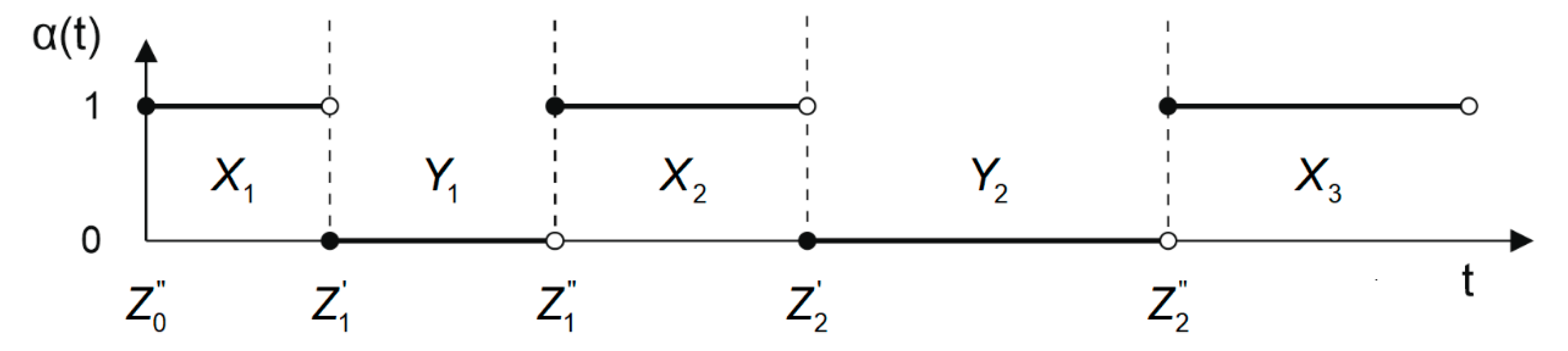
2.2. Mathematical Model

In order to solve the deformation diagnostic problems, stocktaking and planning engineering work on the railways (with the use of RTK GNSS measurements), it is necessary to ensure the accuracy of the GNSS receiver’s positioning. Apart from the accuracy, it is equally important to ensure the availability of a position which meets the requirements for maximally permissible position errors. It was assumed that an availability exceeding 95% of the measurement time is necessary to perform such tasks in practice.
In order to determine, by experimental measurements, the actual availability of GNSS systems as a function of the network type (GPS, GPS/GLONASS and GPS/GLONASS/Galileo), it is necessary to develop a mathematical model that enables determination of the availability for three levels of position errors. Let us assume that the maximum acceptable position errors in the RTK application are 1 cm (p = 0.95) for the rail deformation diagnostics, 3 cm (p = 0.95) for the stocktaking work and 10 cm (p = 0.95) for the design work, which will be designated with the variable U as:
U = { 1   cm   ( p = 0.95 )   for   deformation 3   cm   ( p = 0.95 )   for   stocktaking 10   cm   ( p = 0.95 )   for   design
Assuming that the error of position coordinate determination by the GNSS geodetic receiver is variable in time, according to the general reliability theory, it can be assigned two statuses as a function of time: life, i.e., a status in which the position error is smaller than the arbitrarily established values of three operation types (deformation, stocktaking and design), which is to be expressed as δ n U for the subsequent determinations of n = 1 ,   2 ,   , and the failure time in which an opposite relationship, δ n > U , occurs. Let us also assume that the values X 1 ,   X 2 ,   correspond to the durations of life times (a position error below the allowable value according to the operation types), and Y 1 ,   Y 2 ,   correspond to their failure times (a position error above the allowable value according to the operation types). In this way, a consequence of the change in the position error is a change in the operational status of a system, represented by variable α ( t ) (Figure 5). Let us also introduce additional designations, so that the moments of time Z n = X 1 + Y 1 + X 2 + Y 2 + + Y n 1 + X n become moments of failure, while moments Z n = Z n + Y n are moments of renewal. Let us additionally assume that the random variables X i ,   Y i for i =   1 ,   2 ,   are independent, and that the life and failure times have identical distributions [40,41].
Based on these assumptions, we can describe the failure process for a (system) navigation structure as [40,41]:
U = { 1   for   Z n t < Z n + 1 0   for   Z n + 1 t < Z n + 1   for   n = 0 , 1 ,
The status α ( t ) = 1 denotes that at the moment t , the single measurement error was smaller than or equal to the value of the allowable position error U , determined according to Equation (1). Otherwise, for δ n > U , let us assume that the system has a failure status [40,41].
According to [40], the final form of availability is defined as the relationship:
A ( t ) = 1 F ( t ) + 0 t [ 1 F ( t x ) ] d H Φ ( x )
where:
H Φ ( x ) = n = 1 Φ n ( x )
is a function of the renewal stream, constituted by the renewal moments of the navigation system complying with a specific operation type, while Φ n ( t ) is a distribution function of the random variable Z n .
In navigation applications, it is most frequently assumed that the distributions of life and failure times are exponential, hence their probability density functions can be expressed using commonly known formulas [42], such as:
f ( t ) = { λ e λ t   for   t > 0 0   for   t 0
g ( t ) = { μ e μ t   for   t > 0 0   for   t 0
with the following respective distribution functions:
F ( t ) = { 1 e λ t   for   t > 0 0   for   t 0
G ( t ) = { 1 e μ t   for   t > 0 0   for   t 0
where:
  • f ( t ) —life time probability density function;
  • g ( t ) —failure time probability density function;
  • λ —failure rate;
  • μ —renewal rate.
When these assumptions are adopted, the final form of the availability can be noted as [40]:
A exp ( t ) = 1 F ( t ) + 0 t [ 1 F ( t x ) ] d H Φ ( x ) = e λ t + 0 t [ 1 ( 1 e λ ( t x ) ) ] d H Φ ( x )
and for the limit value:
A exp ( t ) = μ λ + μ + λ λ + μ e ( λ + μ ) t
The transition from Equations (9) and (10) was omitted due to the computational complexity. It was presented in detail on pages 35–37 of the publication [40].
The proposed model will be further used for working out the measurement data recorded in real time by five GNSS geodetic receivers during the measurement journeys along the same route. The measurements were divided into three parts, in which RTK corrections from GPS satellites were used initially, then from GPS/GLONASS satellites, and finally from GPS/GLONASS/Galileo satellites.

3. Results

Data sets were obtained, over six journeys, from five receivers of the same type. They recorded the measurement results [point number, measurement time and two-dimensional Cartesian coordinates in the PL-2000 (national coordinate system used in Poland) [43], normal height of a point in the Kronstadt vertical coordinate system (PL-KRON86-NH) [43], DOP (Dilution of Precision), NoS and mean error of the horizontal and vertical coordinates], saving them as text files. Each receiver recorded three measurement files, which refer to measurements made with RTK corrections in the following variants: GPS, GPS/GLONASS and GPS/GLONASS/Galileo.
In the next stage of measurement data preparation, measurements from five receivers of the same type were brought into common time intervals (all receivers had to register position data within a set period of time). Table 2 presents the times of starting and finishing measurements by receivers T1–T5 at three settings (GPS, GPS/GLONASS and GPS/GLONASS/Galileo). Each measurement included two full rounds of the test loop.
The following part of the paper presents an analysis of the receivers of the T producer. Subsequently, the measurement results were worked out statistically. This was done to determine the mean values of three parameters, the mean value of the NoS used, and the mean and minimum PDOP value. The aim was to compare those values for three GNSS solutions (GPS, GPS/GLONASS and GPS/GLONASS/Galileo). The results are presented in Table 3 and Table 4.
The results presented in Table 3 compare the selected parameters from two measurement series, taken, with RTK corrections, in the following variants: GPS and GPS/GLONASS. They show clearly that the use of the GNSS geodetic network, which sends corrections from two systems (GPS/GLONASS) rather than from one (GPS), improves greatly the satellite signal availability. The NoS increased by five, on average, which accounts for 76.82% of the constellation. As an obvious consequence of the situation, the mean PDOP coefficient decreased by 8.83%.
Another comparison of the selected parameters (PDOP and mean NoS) was used for the measurements where the GPS/GLONASS and GPS/GLONASS/Galileo solutions were employed (Table 4).
The statistical results presented here increased the mean number of the available satellites by two, which corresponds to an increase of 15.99%. However, analyses of the mean value of the PDOP are apparently surprising, because an increase in the NoS used in the measurements should result in a decrease in the mean PDOP [44]. In the conducted studies, the reverse tendency occurred such that, despite the increase in the NoS (from 11.38 to 13.2), the mean PDOP increased (from 2.38 to 2.87), which resulted in the deterioration of the positioning accuracy of the two-system solution (GPS/GLONASS) compared to the three systems (GPS/GLONASS/Galileo). The process of seeking the cause of this involved sorting the PDOP values for the GPS/GLONASS and GPS/GLONASS/Galileo solutions (Figure 6).
The tables show that use of three systems created such geometric conditions, with regards to the signal reception, that many more measurements of large PDOP values appeared, which had a decisive impact on the mean PDOP, determined in Table 4.
The main aim of this study is to determine the positioning availability at three levels of accuracy, 1 cm (deformation) 3 cm (stocktaking) and 10 cm (design), for three operation modes of the GNSS system, GPS, GPS/GLONASS and GPS/GLONASS/Galileo. The mathematical model developed earlier was used in the analyses. Table 5 shows the examination results for the vertical error in a 1D space.
The following conclusions can be drawn from Table 5 regarding 1D positioning:
  • GPS—No availability for the 1-cm threshold. Low availability for the 3-cm level (38.72%) and high availability for the 10-cm level (94.24%);
  • GPS/GLONASS—No availability for the 1-cm threshold. Medium availability for the 3-cm level (79.04%) and high availability for the 10-cm level (98.52%);
  • GPS/GLONASS/Galileo—No availability for the 1-cm threshold. Medium availability for the 3 cm level (78.89%) and high availability for the 10-cm level (97.43%);
  • A considerable increase in availability when two- (GPS/GLONASS) and three-system (GPS/GLONASS/Galileo) solutions are applied, compared to the GPS solution for the 3-cm level;
  • Absence of a significant increase in availability when two- (GPS/GLONASS) or three-system (GPS/GLONASS/Galileo) solutions are applied.
Studies concerning 2D position errors are presented in Table 6.
The following conclusions can be drawn from Table 6 regarding 2D positioning:
  • GPS—No availability for the 1-cm threshold. Medium availability for the 3-cm level (80.27%) and high availability for the 10-cm level (95.91%);
  • GPS/GLONASS—Low availability for the 1-cm threshold. High availability for the 3-cm level (89.03%) and the 10-cm level (99.19%);
  • GPS/GLONASS/Galileo—Low availability for the 1-cm threshold. High availability for the 3-cm level (91.52%) and the 10-cm level (98.63%);
  • A considerable increase in availability when two- (GPS/GLONASS) and three-system (GPS/GLONASS/Galileo) solutions are applied compared to the GPS solution for the 1-cm level;
  • Absence of a significant increase in availability when two- (GPS/GLONASS) or three-system (GPS/GLONASS/Galileo) solutions are applied.
Studies concerning 3D position errors are presented in Table 7.
The following conclusions can be drawn from Table 7 regarding 3D positioning:
  • GPS—No availability for the 1-cm threshold. Low availability for the 3-cm level (17.55%) and high availability for the 10-cm level (92.83%);
  • GPS/GLONASS—No availability for the 1-cm threshold. Medium availability for the 3-cm level (64.65%) and high availability for the 10-cm level (98.12%);
  • GPS/GLONASS/Galileo—No availability for the 1-cm threshold. Medium availability for the 3-cm level (70.69%) and high availability for the 10-cm level (96.48%);
  • A considerable increase in availability when two- (GPS/GLONASS) and three-system (GPS/GLONASS/Galileo) solutions are applied compared to the GPS solution for the 3-cm level;
  • Absence of a significant increase in availability when two- (GPS/GLONASS) or three-system (GPS/GLONASS/Galileo) solutions are applied.

4. Discussion

First, let us consider those parameters which have a considerable impact on the measurement accuracy: the NoS used in positioning and the PDOP values of the measurements. Table 8 shows the graphs presenting these variables as a function of time for five receivers of the T producer (table rows), which were compared with three GNSS solutions, GPS, GPS/GLONASS and GPS/GLONASS/Galileo (table columns).
The results show that the PDOP values for the GPS operation mode, and their variability, are much higher than in the other two cases. Moreover, the NoS used for positioning ranges between five and eight. The PDOP exceeds two most of the time, and a change of the satellites followed (even by one) has a significant impact on the PDOP. It is clear for the GPS/GLONASS and GPS/GLONASS/Galileo solutions that the variability of the NoS followed increases; it is 5–16 for the GPS/GLONASS solution, and as many as 6–20 for the GPS/GLONASS/Galileo solution. Therefore, a fundamental question arises—does adding a third system (Galileo) result in a significant improvement of the measurement accuracy? To this end, 3D, 2D and 1D position errors are analysed as a function of time. Table 9 shows the graphs presenting these variables as a function of time for five receivers of the T producer (table rows), which were compared with the three GNSS solutions, GPS, GPS/GLONASS and GPS/GLONASS/Galileo (table columns).
It is noticeable that 3D, 2D and 1D error positions in the GPS operation mode deviate considerably from the other results for the GPS/GLONASS and GPS/GLONASS/Galileo modes. On the other hand, two- and three-system solutions ensure lower values and variability. A comparison of results from the GPS/GLONASS and GPS/GLONASS/Galileo solutions shows that they are very similar. Insignificant differences (to the advantage of the GPS/GLONASS/Galileo solution) can be noted in the measurements from 800 s to 1300 s, where the three-system solution gives slightly smaller errors in a moderately urbanised area.
Based on the analyses and research carried out, the following conclusions can be drawn:
  • 3D analysis—application of a two- or three-system GNSS solution considerably increases the positioning availability for the 3-cm threshold compared to the GPS solution, by 47.1% for GPS/GLONASS and 53.14% for GPS/GLONASS/Galileo;
  • 2D analysis—two- or three-system GNSS solutions considerably increase the positioning availability for the 1-cm threshold, by 19.61% for GPS/GLONASS and 35.56% for GPS/GLONASS/Galileo. Moreover, the application of the GPS/GLONASS/Galileo solution considerably increases (by 15.95%) the positioning availability for the 1-cm threshold, compared to the GPS/GLONASS solution;
  • 1D analysis—it is worth using multi-GNSS receivers in height measurements, because the positioning availability for the 3-cm threshold considerably increased compared to the GPS solution. A two- and three-system GNSS solution considerably increases the positioning accuracy, compared to the GPS solution, by approximately 40%;
  • Absence of a significant increase in availability when two- (GPS/GLONASS) or three-system (GPS/GLONASS/Galileo) solutions are applied for 3D, 2D and 1D positioning.

5. Conclusions

This study has shown that the rapid development of GNSS techniques, manifesting itself in recent years in the construction of new positioning systems and the modernisation of existing ones, as well as the implementation of new technical solutions for satellite positioning, makes them usable for increasingly precise position determination, also in the kinematic mode.
The study has confirmed that using additional positioning systems is justified. According to a well-known rule, each new satellite increases the measurement availability and the solution reliability. This effect is also clearly noticeable in the current study, in the transition from one-system GPS solution to the two-system GPS/GLONASS one. However, it is much less noticeable in the transition from a two-system to a three-system GPS/GLONASS/Galileo solution. This stems from the fact that these are independent systems, with systematic differences between them. Moreover, Galileo is a new system compared to the other two, it is still under construction, and as such it is not yet fully operational.
To sum up, the most important benefits of using a multi-GNSS system over a single-GNSS solution are:
  • It improves the solution availability in signal-obstructed areas, such as urban canyons, or when a GNSS receiver is not ideally located on the object being positioning, e.g., inside a car [44,45,46];
  • It reduces DOP values, which results in more accurate position estimates [47]. For example, doubling the NoS can decrease the DOP value by 29% [44];
  • Using more satellites will enhance the statistical reliability of the system. This means that the multi-GNSS solution is more likely (in terms of probability) to identify a measurement blunder of a certain magnitude than is a single-GNSS solution [44];
  • It improves the Time to First Fix (TTFF), a measure of the time needed for a GNSS receiver to determine its location [46].

Author Contributions

Conceptualization, M.S. and C.S.; Data curation, L.S., K.C. and J.S. (Jacek Skibicki); Formal analysis, L.S. and K.C.; Investigation, P.C., J.S. (Jacek Szmagliński) and S.G.; Methodology, A.W., W.K. and J.S. (Jacek Skibicki); Software, K.K. and S.J.; Supervision, A.W. and W.K.; Validation, P.C. and J.S. (Jacek Szmagliński); Visualization, P.S.D. and S.G.; Writing—original draft, M.S., C.S. and P.S.D.; Writing—review and editing, K.K. and S.J. All authors have read and agreed to the published version of the manuscript.

Funding

This research was funded by the National Centre for Research and Development in Poland and the PKP Intercity, grant number POIR.04.01.01-00-0017/17.

Conflicts of Interest

The authors declare no conflict of interest.

References

  1. ACIL Allen Consulting. Precise Positioning Services in the Rail Sector. Available online: http://www.ignss.org/LinkClick.aspx?fileticket=rpl6BIao%2F54%3D&tabid=56 (accessed on 30 June 2020).
  2. Barbu, G.; Marais, J. The SATLOC Project. In Proceedings of the Transport Research Arena 2014 (TRA2014), Paris, France, 14–17 April 2014. [Google Scholar]
  3. Junting, L.; Jianwu, D.; Yongzhi, M. NGCTCS: Next-generation Chinese Train Control System. J. Eng. Sci. Technol. Rev. 2016, 9, 122–130. [Google Scholar] [CrossRef]
  4. Ning, B.; Tang, T.; Qiu, K.; Gao, C.; Wang, Q. CTCS—Chinese Train Control System. Adv. Train Control Syst. 2010, 46. [Google Scholar] [CrossRef]
  5. Albanese, A.; Marradi, L.; Campa, L.; Orsola, B. The RUNE Project: Navigation Performance of GNSS-based Railway User Navigation Equipment. In Proceedings of the 2nd ESA Workshop on Satellite Navigation User Equipment Technologies (NAVITEC 2004), Noordwijk, The Netherlands, 8–10 December 2004. [Google Scholar]
  6. Betts, K.M.; Mitchell, T.J.; Reed, D.L.; Sloat, S.; Stranghoener, D.P.; Wetherbee, J.D. Development and Operational Testing of a Sub-meter Positive Train Location System. In Proceedings of the 2014 IEEE/ION Position, Location and Navigation Symposium (PLANS 2014), Monterey, CA, USA, 5–8 May 2014. [Google Scholar]
  7. Marais, J.; Beugin, J.; Berbineau, M. A Survey of GNSS-based Research and Developments for the European Railway Signaling. IEEE Trans. Intell. Transp. Syst. 2017, 18, 2602–2618. [Google Scholar] [CrossRef] [Green Version]
  8. Specht, C.; Smolarek, L.; Pawelski, J.; Specht, M.; Dąbrowski, P. Polish DGPS System: 1995–2017—Study of Positioning Accuracy. Pol. Marit. Res. 2019, 26, 15–21. [Google Scholar] [CrossRef] [Green Version]
  9. Krasuski, K.; Ćwiklak, J.; Jafernik, H. Aircraft Positioning Using PPP Method in GLONASS System. Aircr. Eng. Aerosp. Technol. 2018, 90, 1413–1420. [Google Scholar] [CrossRef]
  10. Specht, C.; Koc, W.; Chrostowski, P.; Szmagliński, J. Accuracy Assessment of Mobile Satellite Measurements in Relation to the Geometrical Layout of Rail Tracks. Metrol. Meas. Syst. 2019, 26, 309–321. [Google Scholar] [CrossRef]
  11. Specht, M.; Specht, C.; Lasota, H.; Cywiński, P. Assessment of the Steering Precision of a Hydrographic Unmanned Surface Vessel (USV) along Sounding Profiles Using a Low-cost Multi-Global Navigation Satellite System (GNSS) Receiver Supported Autopilot. Sensors 2019, 19, 3939. [Google Scholar] [CrossRef] [Green Version]
  12. Szot, T.; Specht, C.; Specht, M.; Dabrowski, P.S. Comparative Analysis of Positioning Accuracy of Samsung Galaxy Smartphones in Stationary Measurements. PLoS ONE 2019, 14, e0215562. [Google Scholar] [CrossRef]
  13. Chrzan, M.; Jackowski, S. Modern Navigation Systems in Rail Transport; Kazimierz Pułaski University of Technology and Humanities in Radom Publishing House: Radom, Poland, 2016. (In Polish) [Google Scholar]
  14. Koc, W.; Specht, C.; Chrostowski, P.; Szmagliński, J. Analysis of the Possibilities in Railways Shape Assessing Using GNSS Mobile Measurements. MATEC Web Conf. 2019, 262, 11004. [Google Scholar] [CrossRef]
  15. Specht, C.; Koc, W. Mobile Satellite Measurements in Designing and Exploitation of Rail Roads. Transp. Res. Procedia 2016, 14, 625–634. [Google Scholar] [CrossRef] [Green Version]
  16. Koc, W.; Specht, C. Results of Satellite Measurements of Railway Track. TTS Rail Transp. Tech. 2009, 7, 58–64. (In Polish) [Google Scholar]
  17. Koc, W.; Specht, C.; Jurkowska, A.; Chrostowski, P.; Nowak, A.; Lewiński, L.; Bornowski, M. Determining the Course of the Railway Route by Means of Satellite Measurements. In Proceedings of the 2nd Scientific-Technical Conference, Design, Construction and Maintenance of Infrastructure in Rail Transport (INFRASZYN 2009), Zakopane, Poland, 22–24 April 2009. (In Polish). [Google Scholar]
  18. Baran, L.W.; Oszczak, S.; Śledziński, J.; Specht, C. Multifunctional Precise Satellite Positioning System ASG-EUPOS. Available online: http://www.asgeupos.pl/webpg/graph/dwnld/ASG-EUPOS_broszura_200806.pdf (accessed on 30 June 2020). (In Polish).
  19. Specht, C.; Mania, M.; Skóra, M.; Specht, M. Accuracy of the GPS Positioning System in the Context of Increasing the Number of Satellites in the Constellation. Pol. Marit. Res. 2015, 22, 9–14. [Google Scholar] [CrossRef] [Green Version]
  20. Specht, C.; Specht, M.; Dąbrowski, P. Comparative Analysis of Active Geodetic Networks in Poland. In Proceedings of the 17th International Multidisciplinary Scientific GeoConference (SGEM 2017), Albena, Bulgaria, 27 June–6 July 2017. [Google Scholar] [CrossRef]
  21. Specht, C.; Koc, W.; Chrostowski, P. Computer-aided Evaluation of the Railway Track Geometry on the Basis of Satellite Measurements. Open Eng. 2016, 6, 125–134. [Google Scholar] [CrossRef] [Green Version]
  22. Specht, C.; Koc, W.; Smolarek, L.; Grządziela, A.; Szmagliński, J.; Specht, M. Diagnostics of the Tram Track Shape with the Use of the Global Positioning Satellite Systems (GPS/GLONASS) Measurements with a 20 Hz Frequency Sampling. J. Vibroeng. 2014, 16, 3076–3085. [Google Scholar]
  23. Koc, W. Design of Rail-track Geometric Systems by Satellite Measurement. J. Transp. Eng. 2012, 138, 114–122. [Google Scholar] [CrossRef]
  24. Koc, W. The Analytical Design Method of Railway Route’s Main Directions Intersection Area. Open Eng. 2016, 6, 1–9. [Google Scholar] [CrossRef]
  25. Koc, W.; Chrostowski, P. Computer-aided Design of Railroad Horizontal Arc Areas in Adapting to Satellite Measurements. J. Transp. Eng. 2014, 140. [Google Scholar] [CrossRef]
  26. Gikas, V.; Daskalakis, S. Determining Rail Track Axis Geometry Using Satellite and Terrestrial Geodetic Data. Surv. Rev. 2008, 40, 392–405. [Google Scholar] [CrossRef]
  27. Chen, Q.; Niu, X.; Zhang, Q.; Cheng, Y. Railway Track Irregularity Measuring by GNSS/INS Integration. Annu. Navig. 2015, 62, 83–93. [Google Scholar] [CrossRef]
  28. Chen, Q.; Niu, X.; Zuo, L.; Zhang, T.; Xiao, F.; Liu, Y.; Liu, J. A Railway Track Geometry Measuring Trolley System Based on Aided INS. Sensors 2018, 18, 538. [Google Scholar] [CrossRef] [Green Version]
  29. Akpinar, B.; Gulal, E. Multisensor Railway Track Geometry Surveying System. IEEE Trans. Instrum. Meas. 2012, 61, 190–197. [Google Scholar] [CrossRef]
  30. Gao, Z.; Ge, M.; Li, Y.; Shen, W.; Zhang, H.; Schuh, H. Railway Irregularity Measuring Using Rauch–Tung–Striebel Smoothed Multi-sensors Fusion System: Quad-GNSS PPP, IMU, Odometer, and Track Gauge. GPS Solut. 2018, 22, 1–14. [Google Scholar] [CrossRef]
  31. Kurhan, M.B.; Kurhan, D.M.; Baidak, S.Y.; Khmelevska, N.P. Research of Railway Track Parameters in the Plan Based on the Different Methods of Survey. Nauka Prog. Transp. 2018, 2, 77–86. [Google Scholar] [CrossRef] [Green Version]
  32. Li, Q.; Chen, Z.; Hu, Q.; Zhang, L. Laser-aided INS and Odometer Navigation System for Subway Track Irregularity Measurement. J. Surv. Eng. 2017, 143, 04017014. [Google Scholar] [CrossRef]
  33. Zhou, Y.; Chen, Q.; Niu, Q. Kinematic Measurement of the Railway Track Centerline Position by GNSS/INS/Odometer Integration. IEEE Access 2019, 7, 157241–157253. [Google Scholar] [CrossRef]
  34. Jiang, Q.; Wu, W.; Jiang, M.; Li, Y. A New Filtering and Smoothing Algorithm for Railway Track Surveying Based on Landmark and IMU/Odometer. Sensors 2017, 17, 1438. [Google Scholar] [CrossRef] [PubMed]
  35. Jiang, Q.; Wu, W.; Li, Y.; Jiang, M. Millimeter Scale Track Irregularity Surveying Based on ZUPT-aided INS with Sub-decimeter Scale Landmarks. Sensors 2017, 17, 2083. [Google Scholar] [CrossRef] [PubMed] [Green Version]
  36. Dąbrowski, P.S.; Specht, C.; Koc, W.; Wilk, A.; Czaplewski, K.; Karwowski, K.; Specht, M.; Chrostowski, P.; Szmagliński, J.; Grulkowski, S. Installation of GNSS Receivers on a Mobile Railway Platform—Methodology and Measurement Aspects. Sci. J. Marit. Univ. Szczec. 2019, 60, 18–26. [Google Scholar] [CrossRef]
  37. Dąbrowski, P.S.; Specht, C.; Felski, A.; Koc, W.; Wilk, A.; Czaplewski, K.; Karwowski, K.; Jaskólski, K.; Specht, M.; Chrostowski, P.; et al. The Accuracy of a Marine Satellite Compass under Terrestrial Urban Conditions. J. Mar. Sci. Eng. 2020, 8, 18. [Google Scholar] [CrossRef] [Green Version]
  38. VRSNet.pl. VRSNet.pl—Reference Station Network. Available online: http://vrsnet.pl/ (accessed on 30 June 2020). (In Polish).
  39. Trimble. Trimble Access Field Software. Available online: https://www.trimble.com/survey/trimble-access-is-monitoring.aspx (accessed on 30 June 2020).
  40. Specht, C. Availability, Reliability and Continuity Model of Differential GPS Transmission. Annu. Navig. 2003, 5, 1–85. [Google Scholar]
  41. Specht, M. Method of Evaluating the Positioning System Capability for Complying with the Minimum Accuracy Requirements for the International Hydrographic Organization Orders. Sensors 2019, 19, 3860. [Google Scholar] [CrossRef] [Green Version]
  42. Barlow, R.E.; Proschan, F. Statistical Theory of Reliability and Life Testing: Probability Models; Holt, Rinehart and Winston: New York, NY, USA, 1974. [Google Scholar]
  43. Council of Ministers of the Republic of Poland. Ordinance of the Council of Ministers of 15 October 2012 on the National Spatial Reference System; Council of Ministers of the Republic of Poland: Warsaw, Poland, 2012. (In Polish) [Google Scholar]
  44. Petovello, M. Would You Prefer to Have More Signals or More Satellites. Inside GNSS 2017, 2017, 45–47. [Google Scholar]
  45. Reuper, B.; Becker, M.; Leinen, S. Benefits of Multi-constellation/Multi-frequency GNSS in a Tightly Coupled GNSS/IMU/Odometry Integration Algorithm. Sensors 2018, 18, 3052. [Google Scholar] [CrossRef] [Green Version]
  46. Telit. The Business Advantages of a Multi GNSS Set-up. Available online: https://www.telit.com/blog/multi-gnss-business-advantages/ (accessed on 30 June 2020).
  47. Elmasry, O.; Tamazin, M.; Elghamarawy, H.; Karaim, M.; Noureldin, A.; Khedr, M. Examining the Benefits of Multi-GNSS Constellation for the Positioning of High Dynamics Air Platforms under Jamming Conditions. In Proceedings of the 2018 11th International Symposium on Mechatronics and its Applications (ISMA), Sharjah, UAE, 4–6 March 2018. [Google Scholar]
Figure 1. Mobile Measurement Platform (MMP) (a) with the layout of the measuring devices (b).
Energies 13 03646 g001aEnergies 13 03646 g001b
Figure 2. The diagram of the MMP: 1—rails, 2—points of forced centring of a Global Navigation Satellite System (GNSS) receiver, 3—platform wheels, di—distances between the GNSS centring points.
Energies 13 03646 g002
Figure 3. The MMP (a), mounting frames of GNSS receivers (b), L manufacturer’s receiver (c) and T manufacturer’s receiver (d).
Energies 13 03646 g003
Figure 4. The layout of the test loop (a) divided into different measurement sections: sections A and B—open area (b), sections C and F—typical urban development (c) and densely built-up sections D and E (d).
Energies 13 03646 g004
Figure 5. The operational statuses: life (a system’s ability to satisfy the positioning requirements for operation types) and failure (an opposite event). Own study based on: [40].
Energies 13 03646 g005
Figure 6. Sorted values of PDOP (the largest values at the table bottom) for the GPS/GLONASS (a) and GPS/GLONASS/Galileo measurements (b).
Energies 13 03646 g006
Table 1. The technical details of the GNSS receivers used in the study.
ParameterL ReceiverT Receiver
Signal trackingGPS: L1, L2, L2C, L5
GLONASS: L1, L2, L2C, L3
BDS: B1, B2, B3
Galileo: E1, E5A, E5B, AltBOC, E6
SBAS: EGNOS, GAGAN, MSAS, QZSS, WAAS
GPS: L1C/A, L1C, L2C, L2E, L5
GLONASS: L1C/A, L1P, L2C/A, L2P, L3
BDS: B1, B2, B3
Galileo: E1, E5A, E5B, E5 AltBOC
SBAS: EGNOS, GAGAN, MSAS, QZSS, WAAS
Real Time Kinematic (RTK) accuracySingle baseline: Hz 8 mm + 1 ppm/V 15 mm + 1 ppm
Network RTK: Hz 8 mm + 0.5 ppm/V 15 mm + 0.5 ppm
Single baseline < 30 km: Hz 8 mm + 1 ppm Root Mean Square (RMS)/V 15 mm + 1 ppm RMS
Network RTK: Hz 8 mm + 0.5 ppm RMS/V 15 mm + 0.5 ppm RMS
Post-processing accuracyStatic with long observations: Hz 3 mm + 0.1 ppm/V 3.5 mm + 0.4 ppm
Static and rapid static: Hz 3 mm + 0.5 ppm/V 5 mm + 0.5 ppm
Static GNSS surveying, high-precision: Hz 3 mm + 0.1 ppm RMS/V 3.5 mm + 0.4 ppm RMS
Static and fast static: Hz 3 mm + 0.5 ppm RMS/V 5 mm + 0.5 ppm RMS
Table 2. Time of starting and finishing measurements by the GNSS receivers (T1–T5), based on which the common time interval, was determined.
Measurement TimeNumber of GNSS Receiver of Manufacturer TCommon Measurement Time for T1–T5
T1T2T3T4T5
GPS
Beginning01:11:0501:10:5201:11:1101:11:1401:11:1801:11:18
End01:50:5901:51:0201:51:0601:51:3701:51:5001:51:50
GPS/GLONASS
Beginning02:42:2802:42:1302:42:3202:42:3602:42:3502:42:36
End03:23:0703:23:0503:23:1203:23:1803:23:1303:23:18
GPS/GLONASS/Galileo
Beginning02:01:2502:01:0602:01:1902:01:1702:01:1402:01:25
End02:31:5102:31:3602:31:5502:31:5802:31:5902:31:59
Table 3. The mean and minimum Position Dilution of Precision (PDOP) and the Number of Satellites (NoS) used by the five GNSS geodetic receivers (T1–T5) in measurements during the journeys, with the use of RTK corrections from Global Positioning System (GPS) and GPS/Global Navigation Satellite System (GLONASS) satellites.
GPSGPS/GLONASS
ParameterT1T2T3T4T5MeanT1T2T3T4T5Mean
Mean PDOP2.412.53.372.392.362.612.512.22.72.212.26 Energies 13 03646 i001 2.38 (−8.83%)
Min. PDOP1.91.91.91.91.91.91.21.21.21.21.2 Energies 13 03646 i001 1.2 (−36.84%)
Mean NoS6.616.55.836.596.656.4411.311.511.011.611.5 Energies 13 03646 i002 11.38 (+76.82%)
Table 4. The mean and minimum PDOP and the NoS used by the five GNSS geodetic receivers (T1–T5) in measurements during the journeys, with the use of RTK corrections, from GPS/GLONASS and GPS/GLONASS/Galileo satellites.
GPS/GLONASSGPS/GLONASS/Galileo
ParameterT1T2T3T4T5MeanT1T2T3T4T5Mean
Mean PDOP2.512.22.72.212.262.382.622.842.682.73.5 Energies 13 03646 i002 2.87 (+20.71%)
Min. PDOP1.21.21.21.21.21.21.21.21.21.21.4 Energies 13 03646 i002 1.24 (+3.33%)
Mean NoS11.311.511.011.611.511.381414131411 Energies 13 03646 i002 13.2 (+15.99%)
Table 5. Availability of 1D positions with errors not exceeding 1 cm, 3 cm and 10 cm for the three positioning solutions, GPS, GPS/GLONASS and GPS/GLONASS/Galileo.
GNSS SolutionMax ErrorAvailability of a 1D Position [%]Relative Availability [+/− %]
T1T2T3T4T5MeanGPS vs. GPS/GLOGPS vs. GPS/GLO/GalGPS/GLO vs. GPS/GLO/Gal
GPS1 cm000000
3 cm56.4940.352.3721.1323.3338.72
10 cm95.6493.988.4895.4897.7194.24
GPS/GLONASS1 cm0000000
3 cm82.7974.7676.5481.679.579.04 Energies 13 03646 i002 40.32
10 cm98.5698.5698.3398.8598.2898.52 Energies 13 03646 i002 4.28
GPS/GLONASS/Galileo1 cm000000 00
3 cm90.9473.5273.5379.5276.9578.89 Energies 13 03646 i002 40.17 Energies 13 03646 i001 −0.15
10 cm99.6597.9197.1898.9293.4797.43 Energies 13 03646 i002 3.19 Energies 13 03646 i001 −1.09
Table 6. Availability of 2D positions with errors not exceeding 1 cm, 3 cm and 10 cm for the three positioning solutions, GPS, GPS/GLONASS and GPS/GLONASS/Galileo.
GNSS SolutionMax ErrorAvailability of a 2D Position [%]Relative Availability [+/− %]
T1T2T3T4T5MeanGPS vs. GPS/GLOGPS vs. GPS/GLO/GalGPS/GLO vs. GPS/GLO/Gal
GPS1 cm000000
3 cm85.7280.3784.1273.7177.4480.27
10 cm97.7794.2290.7798.1998.6295.91
GPS/GLONASS1 cm26.119.6821.3714.5116.3819.61 Energies 13 03646 i002 19.61
3 cm87.9384.1288.0895.8289.2189.03 Energies 13 03646 i002 8.76
10 cm98.8199.5698.9399.499.2799.19 Energies 13 03646 i002 3.28
GPS/GLONASS/Galileo1 cm51.0629.333.0643.6920.6735.56 Energies 13 03646 i002 35.56 Energies 13 03646 i002 15.95
3 cm97.7988.2688.2392.2591.0991.52 Energies 13 03646 i002 11.25 Energies 13 03646 i002 2.49
10 cm99.8899.399.0899.7195.1898.63 Energies 13 03646 i002 2.72 Energies 13 03646 i001 −0.56
Table 7. Availability of 3D positions with errors not exceeding 1 cm, 3 cm and 10 cm for the three positioning solutions, GPS, GPS/GLONASS and GPS/GLONASS/Galileo.
GNSS SolutionMax ErrorAvailability of a 3D Position [%]Relative Availability [+/− %]
T1T2T3T4T5MeanGPS vs. GPS/GLOGPS vs. GPS/GLO/GalGPS/GLO vs. GPS/GLO/Gal
GPS1 cm000000
3 cm27.9521.0823.097.77.9317.55
10 cm94.7490.7387.6794.2696.7492.83
GPS/GLONASS1 cm0000000
3 cm71.2365.6160.8365.0960.5064.65 Energies 13 03646 i002 47.1
10 cm98.0597.9698.0898.897.7398.12 Energies 13 03646 i002 5.29
GPS/GLONASS/Galileo1 cm000000 00
3 cm74.2666.3567.574.3271.0370.69 Energies 13 03646 i002 53.14 Energies 13 03646 i002 6.04
10 cm99.2596.2496.7298.4191.7696.48 Energies 13 03646 i002 3.65 Energies 13 03646 i001 −1.64
Table 8. The NoS used and PDOP values recorded by five receivers of the T producer for the three GNSS solutions, GPS, GPS/GLONASS and GPS/GLONASS/Galileo.
TGPSGPS/GLONASSGPS/GLONASS/Galileo
1 Energies 13 03646 i003 Energies 13 03646 i004 Energies 13 03646 i005
2 Energies 13 03646 i006 Energies 13 03646 i007 Energies 13 03646 i008
3 Energies 13 03646 i009 Energies 13 03646 i010 Energies 13 03646 i011
4 Energies 13 03646 i012 Energies 13 03646 i013 Energies 13 03646 i014
5 Energies 13 03646 i015 Energies 13 03646 i016 Energies 13 03646 i017
Table 9. 3D, 2D and 1D position errors recorded by five receivers of the T producer for the three GNSS solutions, GPS, GPS/GLONASS and GPS/GLONASS/Galileo.
TGPSGPS/GLONASSGPS/GLONASS/Galileo
1 Energies 13 03646 i018 Energies 13 03646 i019 Energies 13 03646 i020
2 Energies 13 03646 i021 Energies 13 03646 i022 Energies 13 03646 i023
3 Energies 13 03646 i024 Energies 13 03646 i025 Energies 13 03646 i026
4 Energies 13 03646 i027 Energies 13 03646 i028 Energies 13 03646 i029
5 Energies 13 03646 i030 Energies 13 03646 i031 Energies 13 03646 i032

