Rapid Fault Diagnosis of PEM Fuel Cells through Optimal Electrochemical Impedance Spectroscopy Tests

Abstract

The present paper is focused on proposing and implementing a methodology for robust and rapid diagnosis of PEM fuel cells’ faults using Electrochemical Impedance Spectroscopy (EIS). Accordingly, EIS tests have been first conducted on four identical fresh PEM fuel cells along with an aged PEMFC at different current density levels and operating conditions. A label, which represents the presence of a type of fault (flooding or dehydration) or the regular operation, is then assigned to each test based on the expert knowledge employing the cell’s spectrum on the Nyquist plot. Since the time required to generate the spectrum should be minimized and considering the notable difference in the time needed for carrying out EIS tests at different frequency ranges, the frequencies have been categorized into four clusters (based on the corresponding order of magnitude: >1 kHz, >100 Hz, >10 Hz, >1 Hz). Next, for each frequency cluster and each specific current density, while utilizing a classification algorithm, a feature selection procedure is implemented in order to find the combination of EIS frequencies utilizing which results in the highest fault diagnosis accuracy and requires the lowest EIS testing time. For the case of fresh cells, employing the cluster of frequencies with $f>10$ Hz, an accuracy of $98.5\%$ is obtained, whereas once the EIS tests from degraded cells are added to the dataset, the achieved accuracy is reduced to $89.2\%$. It is also demonstrated that, while utilizing the selected pipelines, the required time for conducting the EIS test is less than one second, an advantage that facilitates real-time in-operando diagnosis of water management issues.

1. Introduction

In recent years, scientists and engineers have been making notable efforts to mitigate air pollution and global warming by substituting fossil fuel based power generation systems with renewable and environment-friendly units [1,2]. The transportation and automotive sectors are shifting the production from gasoline to Electric Vehicles (EVs). However, these solutions depend on lithium-ion batteries, which guarantee a low autonomy. Furthermore, the time needed to completely charge the device is too long, if compared to the current refueling time of a generic car [3]. An alternative solution to the latter problem is the adoption of hydrogen as fuel and feeding it into a Polymer Electrolyte Membrane Fuel Cell (PEMFC), an electrochemical device that is able to convert the chemical energy of hydrogen into electrical energy [1]. Unfortunately, these devices are still too expensive (owing to the cost of the employed materials) and their durability does not meet today’s need [4,5,6,7,8,9]. In addition, the device is complex and its operation is strongly dependent on the operating conditions, which need to be maintained in an optimized range as much as possible, in order to guarantee stable and reliable generation [10,11,12,13,14,15]. Working at operation points that are far from the optimal one results in various issues, specifically problems corresponding to water content of the membrane, which should be well-hydrated during the operation. Accordingly, non-optimal water content results in dehydration or flooding faults within the cell [5,10,16,17,18]. Thus, the PEMFC’s health management and diagnostics is an indispensable task to ensure a desirable operation [7,11,19,20].

In this context, Electrochemical Impedance Spectroscopy (EIS) has been determined to be a promising diagnostic tool for recognizing faults and in particular water management related ones [21]. EIS is used to diagnose the cell following mainly two approaches: model-based or data-driven methods [22]. Model-based techniques require a deep knowledge of the system and the inter-relations between the corresponding physical phenomena [23]. Data-driven (non-model-based) methods, are instead based on the data collected in the context of an experimental campaign, which is subsequently analyzed and is then employed in the training procedure [24,25,26,27]. Some recent studies have been dedicated to diagnosing water management faults through EIS. Kurz et al. [28] developed a control strategy based on simultaneous EIS measurements on single cells (6-cell PEMFC stack), to distinguish between flooding and drying conditions. They demonstrated that only two points from the spectrum are necessary to detect the kind of fault that is present: HFR (High Frequency Resistance, 1 kHz) and FIV (Flooding Indication Value, 0.5 Hz). The adopted control strategy was able to prevent any voltage drop half an hour prior to the time required to observe the same phenomenon in the polarization curve [29]. Zheng et al. [30] used EIS and a double-fuzzy method (fuzzy clustering and logic) as an unsupervised machine learning approach to mine diagnostic rules automatically. Wasterlain et al. [31] studied a 20-cells PEMFC stack and investigated flooding/drying phenomena. In this study, six different degrees of flooding and drying were considered (from light drying to moderate flooding) and a Naive Bayes classifier was used to automatically recognize the faults. It was shown that the latter supervised machine learning based approach ensures an accuracy of 91.2%. Fouquet et al. [32] used a model-based diagnosis method, coupled with EIS, to detect the water content of a six-cells PEMFC stack. Furthermore, in the latter study, the equivalent circuit’s parameters were fitted to the data. Petrone et al. [33] carried out several tests on an $H_2$/$O_2$ PEMFC to generate faulty conditions and utilized EIS measurements to determine the main features for diagnosis purposes. Jeppesen et al. [34] proposed a data-driven impedance-based diagnosis methodology for high temperature PEMFC, in which the EIS measurements were labeled based on types of faults (five different labels related to high/low air cathode stoichiometry, CO poisoning, high/low methanol anode stoichiometry). In the latter study, EIS measurements were first pre-processed and some features were then selected to reduce the dimensionality of the problem. Lastly, an Artificial Neural Network (ANN) [35] was employed as the machine learning algorithm and the accuracy of 94.6% (100% for the CO poisoning case and cathode stoichiometry) was obtained.

Recent studies have demonstrated that the EIS testing procedure can be conducted on automotive PEM fuel cells in operation through limited modifications to the converter [36,37]. Such feasibility provides the notable benefit of possible utilization of EIS based methodology as a real-time in-operando diagnostic tool. Nevertheless, in most of the previous studies, the entire EIS spectrum has been utilized as the input, performing the procedure of which requires a notable time that limits the applicability of this method for real-time application.

Motivated by the latter research gap, in the present work, a methodology for real-time fault diagnosis of PEM fuel cells is proposed and implemented, in which results of EIS tests conducted at a reduced number of frequencies (rather than the whole spectrum) can be provided as input features. Accordingly, EIS tests have been first carried out at different current density levels and operating conditions. The presence of flooding or drying phenomena at each test has then been determined employing the cell’s spectrum on the Nyquist plot. Each test and the corresponding spectrum is thus assigned with a label, which represents the presence of a type of fault or regular operation. Considering the fact that the time required to generate the spectrum should be minimized and taking into account the notable difference in the time needed for carrying out the EIS tests at different frequency ranges, the frequencies have been categorized into four clusters (based on the corresponding order of magnitude: >1 kHz, >100 Hz, >10 Hz, >1 Hz). Next, for each frequency cluster and for each specific current density, while employing a machine learning algorithm [38,39,40], a recursive feature elimination procedure is implemented and the set of EIS frequencies employed that result in the highest accuracy and require the lowest EIS testing time are determined. The procedure has firstly been implemented on fresh cells, and then on both fresh and degraded (aged) cells, in order to verify the dependence of the chosen frequencies along with the obtained accuracy on the cell’s age.

It is worth noting that the key contribution of the present paper is selecting frequencies at which the EIS should be performed and determining the resulting accuracy. The obtained results facilitate reducing the required EIS testing time, which in turn permits the application of this methodology in real-time (in-operando) applications.

2. Electrochemical Impedance Spectroscopy

Electrochemical Impedance Spectroscopy (EIS) is a diagnostic tool based on system dynamics: a harmonic voltage (or current) perturbation is superimposed to steady state potential (or current), so that the resulting impedance of the system can be measured in a wide range of frequencies. Solving the problem in a frequency-domain allows to separate different physical phenomena that are occurring in the system [29,41,42]. As such, the fastest phenomena can be shown only if the applied disturbance is fast enough [29,41,43]. Considering a voltage perturbation (Potentiostatic mode) being applied to the system:

$$\Delta V=\Delta V_0+|\Delta V_1|cos\left(\omega t\right)=\Delta V_0+\Re \Delta V_1{e}^{j\omega t}$$

(1)

As shown in (1), the voltage variation is the sum of a steady-state value ($\Delta V_0$) and a sinusoidal oscillation. As a result, the current will adapt to this perturbation, according to (2), with a certain phase-shift $\varphi$:

$$I=I_0+\left|I_1\right|cos(\omega t+\varphi )$$

(2)

Under the hypothesis of linearity of the system, the impedance can be defined as the ratio between the oscillation of voltage and the one of current.

$$Z\left(\omega \right)=\frac{\Delta V_1}{I_1}=Z_{\Re }+j{Z}_{\Im }$$

(3)

From (3), which is a complex number, some information about the modulus and the phase shift can be easily obtained, as follows:

$$\left\{\begin{array}{c}\left|Z\right|=\frac{|\Delta V_1|}{|I_1|}\hfill \\ tan\varphi =\frac{Z_{\Im }}{Z_{\Re }}\hfill \end{array}\right.$$

(4)

After repeating the same calculations for a wide range of frequencies, the result can be plotted in both Bode or Nyquist form. Bode is a ($\left|Z\right|-f$) and ($\varphi -f$) plot, whereas in a Nyquist plot the imaginary part of the impedance is plotted against the real one. The latter is the one used in the following analysis.

2.1. Nyquist Plot

From the analysis of an impedance spectrum in the Nyquist plot, possible PEM fuel cell’s issues can be recognized [29]. Starting from the highest frequencies (left part of the graph, as demonstrated in Figure 1), the intercept of the impedance arc on real axis is called HFR (High Frequency Resistance) and it is the sum of the ionic resistance of the membrane and electric resistances of GDL, MPL, and the bipolar plates. A high frequency arc, related to the hydrogen oxidation reaction (HOR) is present, but it can be hardly seen since the fast kinetics at the anode results in a much smaller capacity element compared to ORR (cathode) reaction. A ${45}^{\circ }$ linear branch is often present in the left part of the Nyquist plot, and it figures out some limitations in the proton-transfer through the CL [31]. Moreover, two capacity loops can be detected: the former is due to kinetics of ORR, the latter is present when there are significant mass transport issues. When the current density increases, size of the first loop becomes smaller and the mass transport capacitive element grows up significantly.

2.2. Water Flooding Issues in Nyquist Plot

The EIS technique can be used to detect flooding or drying issues into PEM fuel cells. When the system suffers from dehydration, the membrane’s ionic conductivity is reduced, the HFR increases and the impedance spectra progressively shifts towards higher real values [10,32]. The ionic conductivity of a PEM rises when the degree of humidification of the membrane is high. In the opposite case, when there is too much water in the cell, the conductivity of the membrane rises (well hydrated membrane, augmented ion transport), but the high content of water blocks the cathode GDL’s pores, hindering mass transport, and reduces the active sites of the CCL. These two effects can be seen in the Nyquist plot: as the water content increases, the real part of the impedance becomes lower, and at the same time the spectrum’s amplitude becomes wider (this last effect can be easily detected looking at both real values and imaginary ones at lower frequencies). The impedance spectra represented in Figure 2 have been obtained by changing cathodic relative humidity ($R{H}_c$), a parameter that can be easily linked to the water content of a PEMFC. At very low current densities ($j=0.2$ A/cm${}^2$), lowering the $R{H}_c$ the fuel cell starts suffering from minor to severe dehydration. At high current densities ($j=1.2$ A/cm${}^2$) instead, the cell becomes more and more flooded when the degree of humidification rises.

2.3. Impedance Spectra of Aged Cells

In addition to the dataset made of EIS spectra obtained from fresh cells, data from an aged cell has also been used. This cell suffers from electrocatalyst degradation, induced through an Accelerated Stress Test (AST), which was performed according to the protocol reported by the US Department of Energy for electrocatalyst degradation. For an ideal electrode, the oxygen reduction kinetics is described by the Tafel law, which is defined as:

$$J=K_r{a}_{O_2}^{\gamma }exp(-\frac{\Delta \mathsf{\Phi }}{b_{ORR}})$$

(5)

where the $K_r$ is the kinetic constant, $a_{o_2}$ is the activity of oxygen, $\gamma$ is the reaction order, $\Delta \mathsf{\Phi }$ is the electrode potential, and $b_{ORR}$ is the Tafel slope. Theoretically, when electrocatalyst degradation occurs, the result is a reduction in the kinetic constant $K_r$, related to a decrease in the Electrochemical Surface Area of the PEMFC. Under the hypothesis of Tafel kinetics for the Oxygen Reduction Reaction, the term $b_{ORR}$ (Tafel-slope) does not change. The Tafel equation is valid when j is far from 0, otherwise a more complex equation (like Butler–Volmer) must be used. The Tafel-slope term is defined as:

$$b_{ORR}=\frac{RT}{\beta F}$$

(6)

In (6), R is the Ideal Gas Constant, T is the absolute temperature, $\beta$ is the symmetry factor (a kinetic parameter) and F is the Faraday constant. Thus, under the hypothesis of fixed current density j, as the Tafel slope is constant, the spectrum remains the same. In fact, the charge transfer resistance $R_{CT}$, for an electrode with ideal oxygen and ion transport, is defined as:

$$R_{CT}=\frac{b}{j}$$

(7)

The resistance is related to the size of the spectrum, and it depends on the ratio of two constant values, therefore the spectrum does not change. It is possible to demonstrate that the latter is valid also when a non-ideal electrode is considered [44]. Theoretically, the fault diagnosis procedure is not affected by this kind of degradation phenomenon, as the spectra should be the same. However, in practice there is a marginal variation between the fresh cell’s spectrum and the aged cell’s one (Figure 3). As already discussed in the literature [45], the latter is associated with the non-uniform degradation of the cathode catalyst layer. This will affect the precision of the implemented pipeline, decreasing the overall classification accuracy.

3. Experiment Description

3.1. System Architecture

Four identical MEAs (Membrane Electrode Assembly) have been tested. The MEA is made up of GDL (Gas Diffusion Layer—SGL29BC), ACL and CCL (Anode and Cathode Catalyst Layers) and the membrane (PEM: Nafion${}^{\circledR }$ XL). Two gaskets with a thickness of 175 $\mathsf{\mu }$m each have been placed between the CCM (Catalyst Coated Membrane, i.e., membrane with catalyst layers) and the graphite plate. The gasket, manually designed by MRT Fuel Cell Lab’s researchers, guarantees a perfect coincidence with MEA’s borders. The assembly ends with the graphite flow-field, current collectors and end-plates connection. The whole structure is kept fixed by six bolts with 12 Nm torque [45]. The system is then connected to the experimental station, which is shown in Figure 4.

The system includes three digital flow meters, used to control gas flow rates (air is fed fully dried, gas purity is estimated to be $99.999\%$ for nitrogen and hydrogen and $99.995\%$ for the oxygen). It also contains three bubblers that are utilized to saturate the inlet gases flow, which set the relative humidity of the flows by controlling the dew point temperature. Furthermore, the set-up comprises pressure transducers—placed at the inlet and at the outlet of the PEMFC (two for the cathode side, and two for the anode one), thermo-couples inserted in specific seats of the tightening plates and connected to an acquisition system. Other employed components include a potentiostat, back-pressure valve (to manage the operating pressure of the system), and the electric load to perform characterization tests (EIS measurements).

Electrochemical Impedance Spectroscopy (EIS) is an electrochemical technique and it has been conducted during the polarization test for each current density. The impedance spectra are characterized by 29 points, each of which is obtained at a specific frequency in the range of 1 Hz to 20 kHz. These measurements did not allow to obtain a complete spectrum in the Nyquist plot (lowe frequencies should be considered). However, using only a part of the spectrum can help reducing the EIS testing time (i.e., time needed to perform the EIS measurements) significantly [44].

3.2. Experimental Procedure

The PEMFC has been firstly initialized following the potentiostatic activation protocol reported in [46]. The cell has then been activated under galvanostatic ($j=0.5$ A/cm${}^2$) reference conditions. The reference conditions are characterized by:

• $T=80$${}^{\circ }$C
• $p=2$$ba{r}_A$
• $R{H}_{anode/cathode}=50\%/30\%$
• Stoichiometry ${\lambda }_{anode/cathode}=2/4$

After twenty minutes of conditioning under steady state operation, the polarization is started (voltage measurement is steady state after ten minutes) and the reference curve is obtained. Once the first test is concluded, the operating parameter that has to be tested can be changed, and after another twenty minutes of conditioning (under steady state operation), the new polarization curve is ready to be obtained. The operating parameters have been changed one by one and in combinations in order to perform a sensitivity analysis aiming at finding out the optimal conditions for the PEMFC (i.e., the one with the highest voltage output, which corresponds to the smallest spectrum in the Nyquist plot). All of the conducted experiments are listed in

Table 1. Experiments carried out with Galvanostatic measurements (for seven different current densities: $j=0.1,0.2,0.5,0.7,1,1.2,1.5$ A/cm${}^2$) and related operating conditions.

Name	Sample	Cell	${\mathit{\lambda }}_{\mathit{a}}$	${\mathit{\lambda }}_{\mathit{c}}$	${\mathbf{RH}}_{\mathit{a}}\%$	${\mathbf{RH}}_{\mathit{c}}\%$	T [${}^{\circ }$C]	p [bar]
EWII B1 REF	1	B1	2	4	50	30	80	2
EWII B1 AN3	2	B1	3	4	50	30	80	2
EWII B1 CA5	3	B1	2	5	50	30	80	2
EWII B1 RHa80	4	B1	2	4	80	30	80	2
EWII B1 RHa100	5	B1	2	4	100	30	80	2
EWII B1 RHc50	6	B1	2	4	50	50	80	2
EWII B1 RHc80	7	B1	2	4	50	80	80	2
EWII B1 RHc100	8	B1	2	4	50	100	80	2
EWII B1 T60	9	B1	2	4	50	30	60	2
EWII B1 HRH P25	10	B1	2	4	80	50	80	2.5
EWII B1 HRH HL P25	11	B1	3	5	80	50	80	2.5
EWII B1 OPT	12	B1	4	8	80	50	80	2.5
EWII B2 REF	13	B2	2	4	50	30	80	2
EWII B2 RHc50	14	B2	2	4	50	50	80	2
EWII B2 RHc80	15	B2	2	4	50	80	80	2
EWII B2 RHc100	16	B2	2	4	50	100	80	2
EWII B3 REF	17	B3	2	4	50	30	80	2
EWII B3 RHc50	18	B3	2	4	50	50	80	2
EWII B3 RHc80	19	B3	2	4	50	80	80	2
EWII B3 RHc100	20	B3	2	4	50	100	80	2
EWII B4 REF	21	B4	2	4	50	50	80	2
EWII B4 RHc50	22	B4	2	4	50	50	80	2
EWII B4 RHc80	23	B4	2	4	50	80	80	2
EWII B4 RHc100	24	B4	2	4	50	100	80	2
EWII B2 REF aged	25	B2	2	4	50	30	80	2
EWII B2 RHc50 aged	26	B2	2	4	50	50	80	2
EWII B2 RHc80 aged	27	B2	2	4	50	80	80	2
EWII B2 RHc100 aged	28	B2	2	4	50	100	80	2

. The experiments have been then repeated in galvanostatic mode for most of the following current densities:

$$\overrightarrow{j}=[0.1,0.2,0.5,0.7,1,1.2,1.5]$$

(8)

As the EIS tests on the above-mentioned cases have not been conducted at all of the mentioned current densities, number of available EIS tests for each current density is different.

Table 2. Number of available fresh and aged cell tests for each current density.

Current Density j [A/cm${}^2$]	Number of Fresh Cell Tests	Number of Aged Cell Tests
0.1	22	1
0.2	22	3
0.5	22	3
0.7	23	3
1.0	22	3
1.2	24	1
1.5	16	1

represents number of the available fresh cell and aged cell tests for each of the considered current densities.

3.3. EIS Testing Time

The required time for conducting the EIS measurements, which is utilized in the implemented feature and algorithm selection procedure, is a limiting factor. The time needed for conducting a measurement at a certain frequency is the inverse of that frequency. Therefore, the total required time is the sum of the inverse values of all of the required frequencies. The obtained value is then multiplied by a constant r, which is an integer number corresponding to the performed repetitions of the sinusoidal oscillation. According to the experience of the co-authors (MRT Fuel Cell Lab), $r=3$ is a reasonable value. The overall required time can thus be estimated as:

$$t=r\sum _{i=1}^{n_{feature}}\frac{1}{f_i}$$

(9)

4. Overall Methodology

As was previously explained, the EIS tests have been conducted in different operating conditions (presented in Table 1) and current densities (reported in Table 2). Since the resulting spectrum for each test includes $m=29$ frequencies and considering the fact that two values ($(Z_{\Re }\left(f_k\right)$ and $Z_{\Im }\left(f_k\right))$) are derived for each frequency $f_k$, the corresponding total number of available features (real and imaginary values) is equal to $2m=58$. 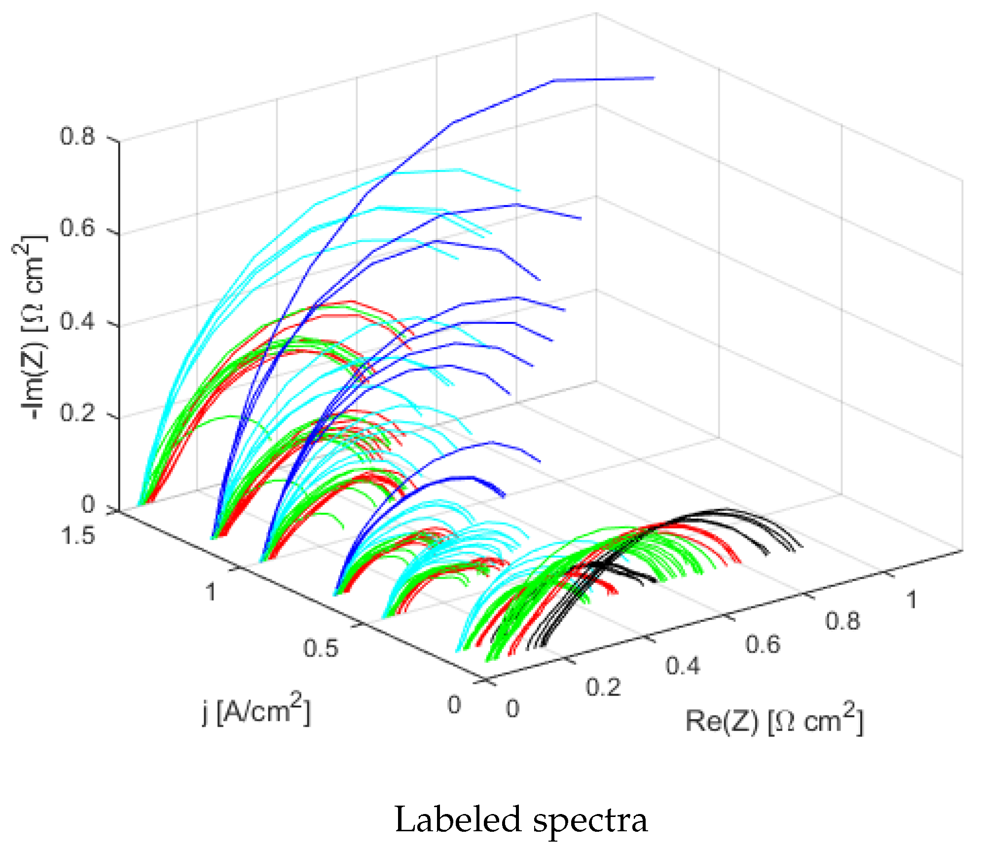A label (which represents the type of fault or regular operation) is assigned to each spectrum based on the corresponding expert knowledge (the experience of laboratory’s research staff gained through experimental activities) employing the cell’s spectrum on the Nyquist plot. The labels which are given to the spectra, as demonstrated in Figure 5, are as follows:

• Regular: the system is working under optimized conditions (or very closed to them).
• Dried: there is evidence of ion conductivity loss, since the spectrum in the Nyquist plot is shifted to the right compared to the regular one.
• Flooded: the spectrum’s amplitude has increased. Positive effect: lower HFR. In fact, while the cathodic GDL’s pores are blocked by water, the membrane conductivity increases due to the high hydration.
• Severely Flooded: same effects of the “Flooded” case, but much more emphasized. This effect can be easily seen at high current densities.
• Severely Dried: very strong dehydration can be detected when current density is very low ($0.1–0.2$ A/cm${}^2$).

As the key aim of the present work is recognizing the potential water management issues (represented by the above-mentioned labels) in PEMFCs employing the EIS spectra, a classification algorithm is provided with the real and imaginary values extracted for each frequency as inputs and is trained to estimate the assigned label (targets). Thus, as the algorithm will only require a spectrum to diagnose the faults, the validity of this procedure can be generalized to any spectrum, independently of the corresponding operating conditions. Linear Discriminant Analysis [47,48,49] is utilized as the classifier in all of the developed pipelines and the corresponding function, provided in the Scikit-learn free software package [50,51], is accordingly employed. As the procedure is implemented for each current density independently, the corresponding number of available EIS spectra (number of tests for each current density that are provided in Table 2) represents the number of rows in the corresponding utilized matrix, while the columns are the imaginary and real values that are obtained at the chosen frequencies (the corresponding selection procedure is explained below). Utilizing the EIS data extracted at a reduced number of frequencies (that would require a lower EIS testing time) facilitates employing the proposed fault diagnosis methodology in a real-time (in-operando) manner. Therefore, a procedure is implemented in order to select set frequencies for each current density, while giving a higher priority to the frequencies with inferior required EIS testing time. Accordingly, considering the notable difference in the time needed for carrying out the EIS tests at different frequency ranges (as explained in Section 3.3), the frequencies are first categorized into four clusters:

• $f>1$ kHz (8 frequencies)
• $f>100$ Hz (15 frequencies)
• $f>10$ Hz (22 frequencies)
• $f>1$ Hz (29 frequencies)

Figure 6 shows the spectra of labeled samples considering the above-mentioned frequency clusters (the axis ranges are kept constant in the sub-figures dedicated to different clusters aiming at demonstrating the relative differences in the corresponding ranges of real and imaginary values).

The overall procedure that is performed for each of the considered frequency clusters is represented in Figure 7. In this procedure, recursive feature elimination is implemented and the accuracy achieved utilizing different combinations of frequencies (using EIS data obtained at these frequencies), is determined. For each set of frequencies, employing the formulation provided in Section 3.3, the corresponding required EIS testing time is then calculated. Next, for each current density, the set of frequencies utilizing which leads to the highest accuracy is determined. In case the highest accuracy can be achieved using multiple pipelines, the one which requires the lowest EIS testing time and the lowest number of frequencies is selected.

The latter procedure is first carried out using a dataset that only includes impedance spectra obtained from PEMFCs in Beginning of Life (BoL) conditions (fresh cells) and then utilizing the data of the EIS tests conducted on both fresh and aged cells.

5. Results and Discussion

5.1. Obtained Results Employing the Data Obtained from Tests Conducted on Fresh Cells

The chosen set of frequencies for each current density along with the resulting accuracy and the determined required EIS testing time, while only employing the cluster of frequencies with $f>1$ kHz, are provided in

Table 3. $f>1$ kHz.

j [A/cm${}^2$]	Accuracy	Required EIS Testing Time [s]	Frequencies [kHz]
0.1	1.0	<${10}^{-3}$	10.1
0.2	1.0	0.0022	1.3
0.5	0.909	0.0039	1.8, 1.3
0.7	0.739	0.0048	14.2, 10.1, 7.2, 1.8, 1.3
1	0.545	<${10}^{-3}$	10.1
1.2	0.583	0.003	3.6, 1.3
1.5	0.688	<${10}^{-3}$	3.6

. As can be observed in this table, for the current densities of $j=0.1$ A/cm${}^2$ and $j=0.2$ A/cm${}^2$, all the labels can be estimated with $100\%$ accuracy. The latter demonstrates that for these current densities, the HFR (High Frequency Resistance) is sufficient to detect the dehydration status of the membrane. Furthermore, as a single elevated frequency is only employed in these selected pipelines, the corresponding required EIS testing time is negligible (<${10}^{-3}$ s). On the other hand, the measurements conducted at kHz frequencies ($f>1$ kHz) do not provide enough information to accurately estimate the labels for higher current densities. For these current densities, an average accuracy of $69\%$ is reached, requiring an average EIS testing time of $0.0025$ s, while six frequencies are required overall.

Considering all of the frequencies higher than 100 Hz, as demonstrated in

Table 4. $f>100$ Hz.

j [A/cm${}^2$]	Accuracy	Required EIS Testing Time [s]	Frequencies [kHz]
0.1	1.0	<${10}^{-3}$	10.1
0.2	1.0	0.0022	1.3
0.5	0.955	0.0197	0.15
0.7	0.739	0.0048	14.2, 10.1, 7.2, 1.8, 1.3
1	0.636	0.0265	10.1, 1.8, 0.12
1.2	0.708	0.0677	14.2, 2.6, 0.30, 0.24, 0.15, 0.12
1.5	0.813	0.0256	14.2, 3.6, 0.12

, the overall achieved accuracy increases (average accuracy: $83.6\%$). For the low current densities ($j=0.1$ A/cm${}^2$ and $j=0.2$ A/cm${}^2$), the accuracy of 100% was already achieved in the previous cluster; thus the selected frequencies for these current densities are identical to the ones of the previous cluster. Similarly, for $j=0.7$ A/cm${}^2$, as a higher accuracy could not be achieved by adding more frequencies, the same frequencies as those of the previous cluster are selected. The accuracy increases for all of the remaining frequencies, nevertheless, several frequencies are required for $j=1.2$ A/cm${}^2$, while an accuracy of only $75\%$ is achieved in this case.

As shown in

Table 5. $f>10$ Hz.

j [A/cm${}^2$]	Accuracy	Required EIS Testing Time [s]	Frequencies [kHz]
0.1	1.0	<${10}^{-3}$	10.1
0.2	1.0	0.0022	1.3
0.5	1.0	0.5263	7.2, 0.15, 0.087, 0.015, 0.011
0.7	0.957	0.4722	7.2, 0.015, 0.011
1	1.0	0.7990	10.1, 0.61, 0.24, 0.12, 0.061, 0.031, 0.022, 0.015, 0.011
1.2	1.0	0.4718	0.015, 0.011
1.5	0.934	0.6305	5.1, 3.7, 0.15, 0.022, 0.015, 0.011

, employing the frequencies higher than 10 Hz is the most promising choice as an accuracy of $100\%$ can be reached for current densities of $j=0.1,$$0.2,$$0.5,$ 1, and $1.2$ A/cm${}^2$, while elevated accuracies can be achieved for the remaining ones ($95.7\%$ for $j=0.7$ A/cm${}^2$ and $93.4\%$ for $j=1.5$ A/cm${}^2$). Using the frequencies that are selected in this cluster, the required EIS testing time for all of the considered current densities is less than one second. These results demonstrate that not all the frequencies need to be considered in order to have an accurate diagnosis and a smaller portion of the spectrum is sufficient.

As demonstrated in

Table 6. $f>1$ Hz.

j [A/cm${}^2$]	Accuracy	Required EIS Testing Time [s]	Frequencies [kHz]
0.1	1.0	$<{10}^{-3}$	10.1
0.2	1.0	0.0022	1.3
0.5	1.0	0.5263	7.2, 0.15, 0.087, 0.015, 0.011
0.7	1.0	0.9532	0.15, 0.0077, 0.0055
1	1.0	0.7990	10.1, 0.61, 0.24, 0.12, 0.031, 0.022, 0.015, 0.011
1.2	1.0	0.4718	0.015, 0.011
1.5	0.934	0.6305	5.1, 3.7, 0.15, 0.022, 0.015, 0.011

, utilizing the selected frequencies, while being provided the whole spectrum, only improves the accuracy at the current density of $j=0.7$ A/cm${}^2$ (from $95.7\%$ to $100\%$). Though, the latter marginal improvement is obtained with the price of increasing the required EIS testing time from $0.47$ s to $0.95$ s. The selected frequencies for the other current densities are identical to the ones obtained for the previous cluster (frequencies higher than 10 Hz). Therefore, it can be concluded at conducting tests at the frequencies between 1 to 10 Hz (which require a notable EIS testing time), does not provide a significant benefit for improving the diagnosis of water management faults.

Table 7. Results of the testing procedure for fresh Electrochemical Impedance Spectroscopy (EIS) data.

Case	Average Accuracy	Average Required EIS Testing Time [s]	Required Frequencies
$f>1$ kHz	0.781	0.0022	6
$f>100$ Hz	0.836	0.0210	11
$f>10$ Hz	0.985	0.4146	15
$f>1$ Hz	0.991	0.4833	16

summarizes the latter discussion by comparing the average accuracy, the average required EIS testing time, and the number of required frequencies corresponding to the selected sets of frequencies of the considered frequency clusters.

Most Influential Frequencies

Figure 8 shows the number of times that the data obtained at a certain frequency is utilized (considering all of the current densities) for each frequency cluster. Thus, it illustrates the most influential frequencies in the selected frequency sets. For the case of $f>10$ Hz, it can be observed that some frequencies ($f=43.6,$$305.18,$$488.28,$$976.56,$$1831,$$2563.5,$ 14160 Hz) are not useful as they are never employed. On the other hand, some of the elevated frequencies including $10132,$$7202,$$3662.1$ and $1342.8$ Hz are selected in all of the considered cases.

5.2. Fresh and Aged Cells

The same procedure, which was previously applied to fresh cells, is then repeated for a dataset including both fresh and aged cells. The latter is conducted in order to assess the dependence of the achieved accuracy and the selected frequencies on cell’s aging.

Table 8. Results of the testing procedure for fresh/aged EIS data.

Case	j [A/cm${}^2$]	Accuracy	Required EIS Testing Time [s]	Frequencies [kHz]
	0.1	1.0	<${10}^{-3}$	10.1
	0.2	0.8	0.0029	14.2, 7.2, 1.3
	0.5	0.8	0.0046	7.2, 5.1, 3.7, 2.6, 1.8
$f>1$ kHz	0.7	0.58	<${10}^{-3}$	7.2
	1	0.44	0.0016	1.8
	1.2	0.4	0.0022	1.3
	1.5	0.76	0.0033	14.2, 5.1, 3.7, 1.8
	0.1	1.0	<${10}^{-3}$	10.1
	0.2	0.88	0.025	14.2, 0.12
	0.5	0.8	0.021	5.1, 2.6, 0.15
$f>100$ Hz	0.7	0.62	0.020	0.15
	1	0.56	0.016	0.15, 0.12
	1.2	0.64	0.022	0.15, 0.12
	1.5	0.88	0.069	14.2, 10.1–5.1, 1.8, 0.98, 0.49, 0.24–0.12
	0.1	1.0	<${10}^{-3}$	10.1
	0.2	0.88	0.025	14.2, 0.12
	0.5	0.88	0.288	5.1, 0.24, 0.011
$f>10$ Hz	0.7	0.88	0.570	0.031, 0.015, 0.011
	1	0.84	0.777	10.1, 5.1, 2.6, 1.8, 0.98–0.061, 0.021, 0.015, 0.011
	1.2	0.88	0.549	0.98, 0.61, 0.15, 0.061, 0.015, 0.011
	1.5	0.88	0.609	0.021, 0.015, 0.011
	0.1	1.0	<${10}^{-3}$	10.1
	0.2	0.88	0.025	14.2, 0.12
	0.5	0.92	0.558	5.1, 0.24, 0.0055
$f>1$ Hz	0.7	0.88	0.570	0.031, 0.015, 0.011
	1	0.88	3.918	0.011, 0.002, 0.0014
	1.2	0.88	0.549	0.98, 0.61, 0.15, 0.061, 0.015, 0.011
	1.5	0.88	0.609	0.021, 0.015, 0.011

summarizes the obtained results for the considered frequency clusters. Considering $f>1$ kHz cluster, the accuracy is lower than the previous case ($68.3\%$ average accuracy vs. $78.1\%$) due to the fact that in the current density range between $0.7$ A/cm${}^2$ to $1.2$ A/cm${}^2$, the accuracy is around $50\%$. However, similar to the previous case, $100\%$ accuracy can be reached for $j=0.1$ A/cm${}^2$, using only one frequency. The classification accuracy increases while more frequencies are considered ($f>100$ Hz), reaching $76.8\%$. To increase the classification accuracy, lower frequencies need to be employed. As such, using $f>10$ Hz results in an average accuracy of $89.2\%$, while requiring an average EIS testing time of less than 0.5 s. The frequencies that are selected while providing the whole spectrum only marginally increase the accuracy to $90.4\%$, while resulting in a higher average EIS testing time ($0.89$ s). Therefore, similar to the previous case, using the cluster of frequencies between 1 to 10 Hz does not provide any significant benefit. For each of the considered frequency clusters, the average accuracy, the average required EIS testing time, and the number of required frequencies corresponding to the selected sets of frequencies are reported in

Table 9. Results of the testing procedure for fresh/aged EIS data.

Case	Average Accuracy	Average EIS Testing Time [s]	Frequencies Required
$f>1$ kHz	0.683	0.00222	8
$f>100$ Hz	0.768	0.032	10
$f>10$ Hz	0.892	0.403	19
$f>1$ Hz	0.904	0.890	17

. Figure 9 shows the number of times that a certain frequency is utilized by the algorithms, for each frequency cluster, demonstrating the most influential frequencies that are selected for the considered current densities.

5.3. Discussion

It was demonstrated using the frequencies that are selected while providing the $f>10$ Hz frequency cluster, an elevated accuracy for the case of fresh cells ($98.5\%$) and an acceptable one ($89.2\%$) for the case of fresh/aged cells can be achieved, while requiring an average EIS testing time of less than 0.5 s in both cases. Therefore, the EIS testing can be conducted at the selected frequencies, while the cell is in operation, and the implemented procedure can be utilized as a real-time approach for diagnosing drying or flooding faults with an acceptable accuracy. It should be pointed out that, although the procedure is conducted at the cell level, the implemented methodology and the determined most influential frequencies can provide helpful insights and guidelines for conducting real-time diagnosis at the stack level.

6. Conclusions

In the present work, a methodology for rapid and robust fault diagnosis of PEM fuel cells utilizing the EIS spectrum was proposed and implemented. In order to reduce the required EIS testing time (which can facilitate utilization of the proposed method in real-time (in-operando) manner), a feature selection procedure was implemented. In this context, considering the notable difference between the required time for conducting EIS tests at different frequencies, the available frequencies were first categorized into four clusters based on the corresponding orders of magnitude. For each frequency cluster and for each specific current density, the achieved accuracy and required EIS testing time of different sets of frequencies were then determined. The frequency set resulting in the highest accuracy and requiring the lowest EIS testing time was then selected for each case. In order to take into account the effect of degradation, the investigation was also carried out using a dataset including both fresh and aged cells.

It was demonstrated that for the fresh cells, through employing the selected frequencies, the faults can be diagnosed with an accuracy of $98.5\%$ while for the fresh/aged cells an accuracy of $89.2\%$ can be achieved. The required EIS testing time in both cases in less than 0.5 s. Therefore, the EIS testing can be conducted at the selected frequencies, while the cell is in operation, and the implemented procedure can be utilized as a real-time strategy for diagnosing drying or flooding faults with an acceptable accuracy. It is worth noting that, although the proposed procedures in the present work are implemented at the cell level, the developed methodology and the determined most influential frequencies can provide helpful insights and guidelines for conducting real-time diagnosis at the stack level. Moreover, since an EIS test conducted at selected frequencies is the only required input in the implemented methodology, the proposed procedure facilitates an accurate diagnosis of water management issues independently of the operating conditions that have caused them.

References

1. Wang, Y.; Chen, K.S.; Mishler, J.; Cho, S.C.; Adroher, X.C. A review of polymer electrolyte membrane fuel cells: Technology, applications, and needs on fundamental research. Appl. Energy 2011, 88, 981–1007. [Google Scholar] [CrossRef] [Green Version]
2. Sharaf, O.Z.; Orhan, M.F. An overview of fuel cell technology: Fundamentals and applications. Renew. Sustain. Energy Rev. 2014, 32, 810–853. [Google Scholar] [CrossRef]
3. Wishart, J. The Vehicle Refueling Wars: A Comparison of Gasoline, Electric, and Fuel Cell Vehicles; FleetCarma Technical Reports; FleetCarma: Waterloo, ON, Canada, 2017. [Google Scholar]
4. Benmouna, A.; Becherif, M.; Depernet, D.; Gustin, F.; Ramadan, H.; Fukuhara, S. Fault diagnosis methods for Proton Exchange Membrane Fuel Cell system. Int. J. Hydrog. Energy 2017, 42, 1534–1543. [Google Scholar] [CrossRef]
5. Zheng, Z.; Petrone, R.; Péra, M.; Hissel, D.; Becherif, M.; Pianese, C.; Steiner, N.Y.; Sorrentino, M. A review on non-model based diagnosis methodologies for PEM fuel cell stacks and systems. Int. J. Hydrog. Energy 2013, 38, 8914–8926. [Google Scholar] [CrossRef]
6. Mohammadi, A.; Djerdir, A.; Steiner, N.Y.; Bouquain, D.; Khaburi, D. Diagnosis of PEMFC for Automotive Application. In Proceedings of the 2015 5th International Youth Conference on Energy (IYCE), Pisa, Italy, 27–30 May 2015; pp. 1–6. [Google Scholar]
7. Sutharssan, T.; Montalvao, D.; Chen, Y.K.; Wang, W.C.; Pisac, C. A review on prognostics and health monitoring of proton exchange membrane fuel cell. Renew. Sustain. Energy Rev. 2017, 75, 440–450. [Google Scholar] [CrossRef] [Green Version]
8. Wu, J.; Yuan, X.Z.; Martin, J.J.; Wang, H.; Zhang, J.; Shen, J.; Wu, S.; Merida, W. A review of PEM fuel cell durability: Degradation mechanisms and mitigation strategies. J. Power Sources 2008, 184, 104–119. [Google Scholar] [CrossRef]
9. Haghighat Mamaghani, A.; Najafi, B.; Casalegno, A.; Rinaldi, F. Long-term economic analysis and optimization of an HT-PEM fuel cell based micro combined heat and power plant. Appl. Therm. Eng. 2016, 99, 1201–1211. [Google Scholar] [CrossRef]
10. Li, H.; Tang, Y.; Wang, Z.; Shi, Z.; Wu, S.; Song, D.; Zhang, J.; Fatih, K.; Zhang, J.; Wang, H.; et al. A review of water flooding issues in the proton exchange membrane fuel cell. J. Power Sources 2008, 178, 103–117. [Google Scholar] [CrossRef]
11. Pahon, E.; Yousfi Steiner, N.; Jemei, S.; Hissel, D.; Moçoteguy, P. A signal-based method for fast PEMFC diagnosis. Appl. Energy 2016, 165, 748–758. [Google Scholar] [CrossRef]
12. Najafi, B.; Haghighat Mamaghani, A.; Rinaldi, F.; Casalegno, A. Long-term performance analysis of an HT-PEM fuel cell based micro-CHP system: Operational strategies. Appl. Energy 2015, 147, 582–592. [Google Scholar] [CrossRef]
13. Haghighat Mamaghani, A.; Najafi, B.; Casalegno, A.; Rinaldi, F. Predictive modelling and adaptive long-term performance optimization of an HT-PEM fuel cell based micro combined heat and power (CHP) plant. Appl. Energy 2017, 192, 519–529. [Google Scholar] [CrossRef]
14. Najafi, B.; Mamaghani, A.; Rinaldi, F.; Casalegno, A. Fuel partialization and power/heat shifting strategies applied to a 30 kWel high temperature PEM fuel cell based residential micro cogeneration plant. Int. J. Hydrog. Energy 2015, 40, 14224–14234. [Google Scholar] [CrossRef]
15. Mamaghani, A.H.; Najafi, B.; Casalegno, A.; Rinaldi, F. Optimization of an HT-PEM fuel cell based residential micro combined heat and power system: A multi-objective approach. J. Clean. Prod. 2018, 180, 126–138. [Google Scholar] [CrossRef]
16. Pei, P.; Li, Y.; Xu, H.; Wu, Z. A review on water fault diagnosis of PEMFC associated with the pressure drop. Appl. Energy 2016, 173, 366–385. [Google Scholar] [CrossRef]
17. Ren, P.; Pei, P.; Li, Y.; Wu, Z.; Chen, D.; Huang, S.; Jia, X. Diagnosis of water failures in proton exchange membrane fuel cell with zero-phase ohmic resistance and fixed-low-frequency impedance. Appl. Energy 2019, 239, 785–792. [Google Scholar] [CrossRef]
18. Najafi, B.; De Antonellis, S.; Intini, M.; Zago, M.; Rinaldi, F.; Casalegno, A. A tri-generation system based on polymer electrolyte fuel cell and desiccant wheel - Part A: Fuel cell system modelling and partial load analysis. Energy Convers. Manag. 2015, 106, 1450–1459. [Google Scholar] [CrossRef]
19. Li, Z.; Outbib, R.; Giurgea, S.; Hissel, D.; Li, Y. Fault detection and isolation for Polymer Electrolyte Membrane Fuel Cell systems by analyzing cell voltage generated space. Appl. Energy 2015, 148, 260–272. [Google Scholar] [CrossRef]
20. Li, Z.; Outbib, R.; Giurgea, S.; Hissel, D.; Jemei, S.; Giraud, A.; Rosini, S. Online implementation of SVM based fault diagnosis strategy for PEMFC systems. Appl. Energy 2016, 164, 284–293. [Google Scholar] [CrossRef]
21. Orazem, M.E.; Tribollet, B. Electrochemical Impedance Spectroscopy; John Wiley & Sons, Inc.: Hoboken, NJ, USA, 2017. [Google Scholar]
22. Chakraborty, U.K. A New Model for Constant Fuel Utilization and Constant Fuel Flow in Fuel Cells. Appl. Sci. 2019, 9, 1066. [Google Scholar] [CrossRef] [Green Version]
23. Polverino, P.; Sorrentino, M.; Pianese, C. A model-based diagnostic technique to enhance faults isolability in Solid Oxide Fuel Cell systems. Appl. Energy 2017, 204, 1198–1214. [Google Scholar] [CrossRef]
24. Wu, X.L.; Xu, Y.W.; Xue, T.; Zhao, D.Q.; Jiang, J.; Deng, Z.; Fu, X.; Li, X. Health state prediction and analysis of SOFC system based on the data-driven entire stage experiment. Appl. Energy 2019, 248, 126–140. [Google Scholar] [CrossRef]
25. Zhang, Z.; Li, S.; Xiao, Y.; Yang, Y. Intelligent simultaneous fault diagnosis for solid oxide fuel cell system based on deep learning. Appl. Energy 2019, 233, 930–942. [Google Scholar] [CrossRef]
26. Chakraborty, U.K. Proton Exchange Membrane Fuel Cell Stack Design Optimization Using an Improved Jaya Algorithm. Energies 2019, 12, 3176. [Google Scholar] [CrossRef] [Green Version]
27. Morán-Durán, A.; Martínez-Sibaja, A.; Rodríguez-Jarquin, J.P.; Posada-Gómez, R.; González, O.S. PEM Fuel Cell Voltage Neural Control Based on Hydrogen Pressure Regulation. Processes 2019, 7, 434. [Google Scholar] [CrossRef] [Green Version]
28. Kurz, T.; Hakenjos, A.; Krämer, J.; Zedda, M.; Agert, C. An impedance-based predictive control strategy for the state-of-health of PEM fuel cell stacks. J. Power Sources 2008, 180, 742–747. [Google Scholar] [CrossRef]
29. Niya, S.M.R.; Hoorfar, M. Study of proton exchange membrane fuel cells using electrochemical impedance spectroscopy technique - A review. J. Power Sources 2013, 240, 281–293. [Google Scholar] [CrossRef]
30. Zheng, Z.; Péra, M.C.; Hissel, D.; Becherif, M.; Agbli, K.S.; Li, Y. A double-fuzzy diagnostic methodology dedicated to online fault diagnosis of proton exchange membrane fuel cell stacks. J. Power Sources 2014, 271, 570–581. [Google Scholar] [CrossRef]
31. Wasterlain, S.; Candusso, D.; Harel, F.; François, X.; Hissel, D. Diagnosis of a Fuel Cell Stack Using Electrochemical Impedance Spectroscopy and Bayesian Networks. In Proceedings of the 2010 IEEE Vehicle Power and Propulsion Conference, Lille, France, 1–3 September 2010; pp. 1–6. [Google Scholar]
32. Fouquet, N.; Doulet, C.; Nouillant, C.; Dauphin-Tanguy, G.; Ould-Bouamama, B. Model based PEM fuel cell state-of-health monitoring via ac impedance measurements. J. Power Sources 2006, 159, 905–913. [Google Scholar] [CrossRef]
33. Petrone, R.; Vitagliano, C.; Péra, M.C.; Chamagne, D. Characterization of an H2/O2 PEMFC Short-Stack Performance Aimed to Health-State Monitoring and Diagnosis. Fuel Cells 2018, 18, 279–286. [Google Scholar] [CrossRef]
34. Jeppesen, C.; Araya, S.S.; Sahlin, S.L.; Thomas, S.; Andreasen, S.J.; Kaer, S.K. Fault detection and isolation of high temperature proton exchange membrane fuel cell stack under the influence of degradation. J. Power Sources 2017, 359, 37–47. [Google Scholar] [CrossRef] [Green Version]
35. Schmidhuber, J. Deep learning in neural networks: An overview. Neural Netw. 2015, 61, 434. [Google Scholar] [CrossRef] [PubMed] [Green Version]
36. Hong, P.; Xu, L.; Jiang, H.; Li, J.; Ouyang, M. A new approach to online AC impedance measurement at high frequency of PEM fuel cell stack. Int. J. Hydrog. Energy 2017, 42, 19156–19169. [Google Scholar] [CrossRef]
37. Kitamura, N.; Manabe, K.; Nonobe, Y.; Kizaki, M. Development of Water Content Control System for Fuel Cell Hybrid Vehicles Based on AC Impedance. Trans. Soc. Autom. Eng. Jpn. 2010, 41, 49–53. [Google Scholar]
38. Hastie, T.; Tibshirani, R.; Friedman, J. The Elements of Statistical Learning; Springer Series in Statistics; Springer: New York, NY, USA, 2001. [Google Scholar]
39. Manivannan, M.; Najafi, B.; Rinaldi, F. Machine learning-based short-term prediction of air-conditioning load through smart meter analytics. Energies 2017, 10, 1905. [Google Scholar] [CrossRef] [Green Version]
40. Najafi, B.; Moaveninejad, S.; Rinaldi, F. Data Analytics for Energy Disaggregation: Methods and Applications. In Big Data Application in Power Systems; Elsevier: Amsterdam, The Netherlands, 2017; pp. 377–408. [Google Scholar]
41. Wu, J.; Yuan, X.Z.; Wang, H.; Blanco, M.; Martin, J.J.; Zhang, J. Diagnostic tools in PEM fuel cell research: Part I Electrochemical techniques. Int. J. Hydrog. Energy 2008, 33, 1735–1746. [Google Scholar] [CrossRef]
42. Brunetto, C.; Moschetto, A.; Tina, G. PEM fuel cell testing by electrochemical impedance spectroscopy. Electr. Power Syst. Res. 2009, 79, 17–26. [Google Scholar] [CrossRef]
43. Yuan, X.Z.; Song, C.; Wang, H.; Zhang, J. Electrochemical Impedance Spectroscopy in PEM Fuel Cells; Springer: Berlin/Heidelberg, Germany, 2010. [Google Scholar]
44. Baricci, A.; Zago, M.; Casalegno, A. Modelling analysis of heterogeneity of ageing in high temperature polymer electrolyte fuel cells: Insight into the evolution of electrochemical impedance spectra. Electrochim. Acta 2016, 222, 596–607. [Google Scholar] [CrossRef]
45. Baricci, A.; Bonanomi, M.; Yu, H.; Guetaz, L.; Maric, R.; Casalegno, A. Modelling analysis of low platinum polymer fuel cell degradation under voltage cycling: Gradient catalyst layers with improved durability. J. Power Sources 2018, 405, 89–100. [Google Scholar] [CrossRef]
46. Yu, H.; Baricci, A.; Casalegno, A.; Guetaz, L.; Bonville, L.; Maric, R. Strategies to mitigate Pt dissolution in low Pt loading proton exchange membrane fuel cell: II. A gradient Pt loading design. Electrochim. Acta 2017, 247, 1169–1179. [Google Scholar] [CrossRef]
47. Tharwat, A.; Gaber, T.; Ibrahim, A.; Hassanien, A.E. Linear discriminant analysis: A detailed tutorial. Ai Communications 2017, 30, 1–22. [Google Scholar] [CrossRef] [Green Version]
48. Brownlee, J. Master Machine Learning Algorithms (Discover How They Work and Implement Them From Scratch). Machine Learning Mastery: Vermont, Australia, 2016. [Google Scholar]
49. Balakrishnama, S.; Ganapathiraju, A. Linear discriminant analysis-a brief tutorial. Inst. Signal Inf. Process. 1998, 18, 1–8. [Google Scholar]
50. Müller, A.C.; Guido, S. Introduction to Machine Learning with Python; O’Reilly Media, Inc.: Sebastopol, CA, USA, 2016. [Google Scholar]
51. Pedregosa, F.; Varoquaux, G.; Gramfort, A.; Michel, V.; Thirion, B.; Grisel, O.; Blondel, M.; Prettenhofer, P.; Weiss, R.; Dubourg, V.; et al. Scikit-learn: Machine Learning in Python. J. Mach. Learn. Res. 2011, 12, 2825–2830. [Google Scholar]
Figure 1. Nyquist plot of a polymer Electrolyte Membrane (PEM) Fuel Cell.
Energies 13 03643 g001
Figure 2. Impedance spectra of dried and flooded PEM fuel cells, at j = 0.2 A/cm 2 and j = 1.2 A/cm 2 respectively.
Energies 13 03643 g002
Figure 3. Comparison between the spectrum of a fresh PEMFC at j = 0.5 A/cm 2 and the spectrum belonging to the same cell with electrocatalyst degradation.
Energies 13 03643 g003
Figure 4. System architecture.
Energies 13 03643 g004
Figure 5. Labeled spectra in a 3D plot. Two of the three axes are the Nyquist plot’s ones (i.e., real and imaginary) and the third is the current density j [A/cm2].
Energies 13 03643 g005
Figure 6. Labeled samples in the Nyquist plot, considering different subsets of frequencies.
Energies 13 03643 g006
Figure 7. Overall methodology explained through a flowchart.
Energies 13 03643 g007
Figure 8. Bar chart showing the most promising features, for each of the four studied frequency clusters. The y-axis represents the absolute frequency for each feature (i.e., number of times that a certain feature appears).
Energies 13 03643 g008
Figure 9. Bar chart showing the most promising features for the fresh/aged case (for all of the considered frequency clusters). The y-axis represents the absolute frequency for each feature (i.e., number of times that a certain feature appears).
Energies 13 03643 g009