Abstract
In this study, a model equation is derived that uses a statistical analysis based on empirical models to predict the airtightness of reinforced concrete apartment buildings popular in Asian regions. Airtightness data from 486 units personally measured by the authors in the past eight years are used. As major variables used in the prediction model, two groups of variables are configured for the geometric components of the envelope, which is a major path of airflow in a building and is where air infiltration and leakage occur. The two groups of variables represent (1) the areas of the individual components forming the envelope and (2) the connection lengths between different components of the envelope. For the effective prediction of airtightness, correlation analysis and multiple regression analysis were applied step by step in this study. The results of the correlation analysis indicated that the areas of the slab and the window are the area variables that present the greatest impact, whereas the perimeter length of the window is the connection length variable that presents the greatest impact. Using a multiple linear regression analysis method, airtightness prediction model equations can be derived, and it is found that the model with variables for area is able to predict airtightness more accurately compared to the two models derived from variables for connection length and all variables for area and connection length. Although the statistical approach in this study shows a limitation in that the prediction results may vary depending on the attributes and type of data collected by countries, the methodology and procedure in this study contribute to similar studies for making prediction models and finding the influence of variables in the future with high applicability and feasibility.
1. Introduction
The airtightness of a building has a significant impact both on the level of indoor air quality and on the durability of the building envelope. In addition, there is growing awareness of the importance of airtightness in a building envelope for reducing the increase in cooling and heating energy costs caused by air infiltration and leakage. As a practical means of ensuring satisfactory levels of airtightness, various building certification schemes entail setting a target airtightness level and conducting direct measurements during the construction stage to check whether or not the target is met [1,2]. Many studies related to the effects of thermal insulation and ventilation on net-zero-energy buildings (NZEBs) have been conducted [3,4]. Moreover, the airtightness performance has been studied as one of the fundamental passive factors in the implementation of NZEBs since it reduces the heating and cooling load of buildings [5]. Data on the airtightness of the envelope, which corresponds to the boundary of the overall building, is inputted beforehand into simulations for evaluating energy performance during the design stages of the building. The input data used for the simulations employ target values, i.e., values that would be desirable for the envelope to reach, or default values, i.e., values that the envelope is expected to reach, rather than measurement values, which can only be obtained after the construction of the building is complete. Thus, it can be said that the determining of airtightness values is of the utmost importance, especially in view of their key role in evaluating environmental and energy performance.
The airtightness values of a fully constructed building are checked by field measurement, often using a pressurization method known as the blower door method [6]. Numerous sets of data measured in a variety of countries have been reported so far [7,8,9,10,11,12,13,14]; based on such data, some studies have analyzed airtightness properties or have presented mathematical models that can estimate airtightness [15]. However, it is not always possible to conduct measurements due to difficulties in preparing measurements (for instance, finding the time available for taking on-site measurements), and there are also many instances in which limitations related to measurement conditions such as weather conditions or building size render measurement difficult. Moreover, numerous tools or certification systems associated with evaluating the energy performance of a building require the airtightness values at the design stages, during which it is impossible to actually measure airtightness. The research conducted by Kondratyev and Varotsos [16] presented numerical modeling efforts considering the climate change factor based on robust and stable observation systems that were required for reliable assessment of the impact of various elements on global climate changes. As such, various studies [11,17,18,19,20,21,22,23,24,25,26] have been conducted that aim to predict the airtightness values of buildings without actual measurements. Various methods for airtightness performance prediction proposed so far in other studies have had a practical limitation in combining construction quality control and workmanship [15], which play a significant role in airtightness performance. Due to this limitation, the prediction methods have not yet presented the accuracy and precision necessary to replace the experimental methodologies based on the actual on-site measurements [22]. The research by Krstić et al. [19] proposed a prediction model of airtightness performance using an artificial neural network (ANN) model based on multilayer perceptron (MLP) theory with four input variables affecting the airtightness performance.
Methods of predicting air infiltration can be divided mainly into theoretical models and empirical models. Theoretical models are based on physical theory and can be grouped into single-zone models and multizone models, whereas empirical models are based on actual measured data [15,21]. In single-zone models, the calculations are made assuming that the air inside is mixed together so that the temperature and pressure are constant at all locations. Typical examples of single-zone models include the Lawrence Berkeley Laboratory model (LBL model) and the Alberta air infiltration model (AIM-2) [27]. In multizone models such as COMIS [28] and CONTAM [29,30], a building is considered to be composed of interconnected spaces, and it is assumed that the air is mixed well within each zone. These models utilize the law of conservation of mass for each zone of the building. However, single-zone models are limited in mostly dealing with low-story buildings (of three stories or lower). On the other hand, multizone models require actual airtightness data on which to base the modeling of airflow, require long periods of time for the modeling, and may provide drastically different results depending on the input data and the levels of experience and understanding on the part of the user [31,32,33].
Empirical models are prediction methods based on actual measured data, and when finding the airtightness of a residential unit, an empirical model uses a statistical analysis of the infiltration rate data of actual residential units [7]. Such data are usually gathered from measurement results obtained by fan pressurization methods, which utilize fans, and tracer gas methods. Feijó-Muñoz et al. [34] proposed the methodology composed of a statistical sampling method with relevant variables such as different typologies, construction years, and climatic zones among collected datasets for the characterization of the envelope airtightness of residential buildings. There are also studies on predicting airtightness by way of regression analysis [10,11,21,24,33]. Wallace et al. [35] investigated the relationships between airtightness and the main driving forces of infiltrations, such as indoor–outdoor temperature difference, wind direction, and wind speed. Prignon et al. [22] reviewed the predictive models and analyzed the relevance of building elements such as the location, age, and size of the building; the number of stories; and the floor area. Factors related to such analyses may also include energy efficiency [10] and management context [11]. In previous studies utilizing empirical models, the measured buildings are mostly single dwellings or small- and medium-sized nonresidential buildings. Various factors are considered, including weather conditions and various building characteristics, but only a limited number of studies consider the geometrical components of the envelope, which is where air infiltration actually takes place.
It has been pointed out that there is a lack of discussion on reproducibility in related studies that predict airtightness in single dwellings or buildings of different construction types [15,26]. However, for residential units built in the form of apartment buildings, it is deemed that prediction is achievable, since the construction techniques or the materials forming the envelopes are similar. In particular, since the airtightness of a building is just another expression for the leakage area of the envelope, it is intuitive that prediction based on the geometrical components of the envelope is easier and more accurate. This study proposes the most effective model among feasible models for predicting the airtightness of residential units based on a statistical analysis of empirical models directed at reinforced concrete apartment buildings constructed mainly in Asia. The variables for the statistical analysis include area variables and connection length variables, which represent the geometrical components of the envelope, where air infiltration and leakage actually occur. The correlation between the airtightness of the overall building and the variables is first analyzed to check the variables’ impact. A multiple linear regression analysis is performed for major variables selected by the impact analysis, whereby an airtightness prediction model is derived that is suitable for residential units of apartment buildings constructed with reinforced concrete.
2. Airtightness Data Collection
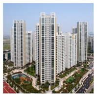
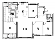
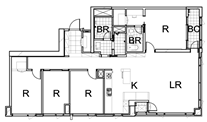
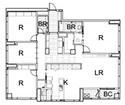
The samples used in the statistical analysis for airtightness prediction are from the airtightness data of 486 residential units in three apartment complexes in Korea measured by the authors. The measuring of airtightness was performed with a pressurization method using a blower door fan as specified by the ASTM-E779 [36]. The measured buildings are high-rise apartment type residential buildings that are located in Korea and were constructed between the years 2008 and 2015. The airtightness values of 210 units from Complex A, 148 units from Complex B, and 128 units from Complex C were measured. The measured buildings are of reinforced concrete and were constructed as punched-window types with balconies formed in the envelope for most units. The apartment complexes generally have floor plans that each includes a core in the center and the residential units positioned around the core in a tower configuration. The dividing partitions between adjoining units are drywalls for Complexes B and C and concrete walls for Complex A. In each complex, the residential units can be grouped according to floor area into 10 types for Complexes A and B and into 15 types for Complex C. As there are about 10 units for each type with different building elements forming the envelope, it was determined that statistical analysis is possible. Information regarding the complexes and residential units measured for this study is summarized below in Table 1.

Table 1.
Test building summary.
After data collection, data exploration based on statistical approaches is required to address the characteristics and attributes of the collected data. The airtightness levels of the 486 units were analyzed based on air change per hour at 50 pascals (ACH50) values. The measurement results for all units of Complexes A, B, and C are represented in Figure 1, while the measurement results for each complex represented are shown in Figure 2. The ACH50 values of the units range from 1.12 to 4.81 h−1 overall, with a mean of 2.59 h−1. Looking at the individual complexes, the ACH50 values range from 1.50 to 4.81 h−1 for Complex A, 1.41 to 3.60 h−1 for Complex B, and 1.12 to 3.79 h−1 for Complex C, with median values of 2.86, 2.30, and 2.45 h−1, respectively. It is observed that the mean ACH50 value for Complex A, which has the smallest mean floor area for the measured units, is somewhat higher compared to the average ACH50 values for Complexes B and C.
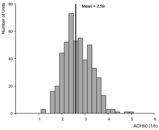
Figure 1.
Airtightness distribution for residential units.
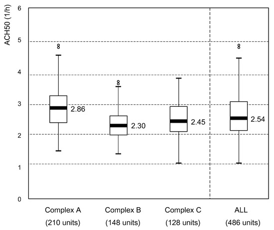
Figure 2.
Airtightness data for each complex.
In order to analyze the correlations between various geometrical components of the envelope and the airtightness value, 486 residential units were divided into types according to floor area. Complexes A and B were each divided into 10 types, while Complex C was divided into 15 types, resulting in a total of 35 floor area types. For each floor area type, there were at least 2 units and at most 50 units measured. The average airtightness value of units corresponding to the same type was used as the representative airtightness value of said type. To increase the reliability of each type’s average value, the ACH50 was recalculated with outliers excluded. Thus, rejecting outliers in each type, the values from 9 out of the 486 units were removed, so that the results of this study are based on the airtightness values of 477 units. The best-estimate airtightness values, in terms of ACH50, before and after excluding outliers for each type grouped according to floor area are summarized in Table 2.

Table 2.
Airtightness data of apartment units based on floor area.
3. Setting Variables for Airtightness Prediction
The previous section introduced descriptive statistics for identifying the attributes and distributions of the raw ACH50 data. The statistical approach makes it possible to analyze the collected raw data and process them into valuable information. Section 3, Section 4 and Section 5 present the statistical relationship between ACH50 and the factors that will be used as independent variables in the prediction model afterwards. The prediction model derived on the basis of this relationship provides the predictive results of ACH50, which vary depending on changes in the factors.
In order to establish a reliable prediction model, which is one of the objectives of this study, investigating factors that have significant influence on ACH50 is required. These factors are used as independent variables of the prediction model. As shown in Figure 3, the residential units of apartment buildings all have similar envelope components. The outer wall of the envelope, including the upper and lower slabs, is all made of reinforced concrete. Every unit has windows connecting to each bedroom and the living room, an entrance to the residential unit, and a louver for ventilating the air-conditioner’s outdoor unit space. The air duct (AD) and pipe duct (PD) rooms, in which the vertically connected ducts and pipes for ventilation and plumbing are installed, are located indoors and surrounded by drywalls. Each residential unit has one kitchen exhaust and two bathroom exhausts installed. The interunit partition walls and the walls at the entrance are made of drywall in the units of Complexes B and C, whereas all of the walls are concrete in the units of Complex A. The development elevations of typical envelopes and the section view of each wall type are shown in Figure 3 and Figure 4. In this study, the geometrical components of the envelope, which is the part of a building where air infiltration and leakage actually take place, were selected as variables in predicting the airtightness of residential units made of reinforced concrete. Two main groups of variables were selected, one being the areas of the individual components forming the envelope, and the other being the connection lengths along which different components forming the envelope are interconnected. Area variables may include the areas of the slab, concrete wall, drywall, window, AD/PD drywall, louver connecting to the air-conditioner outdoor unit space, the entrance door, and the like. Connection length variables may include the connection lengths between a drywall and a drywall, between a concrete wall and a concrete wall, and between a drywall and a concrete wall, as well as the perimeter lengths of the window, the AD/PD drywall, the air-conditioner outdoor unit space louver, and the entrance door, etc.
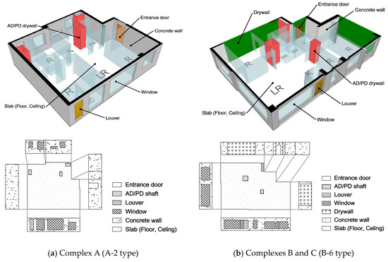
Figure 3.
Typical residential units and envelope development elevations; the dividing partitions between adjoining units are drywalls for Complexes B and C and concrete walls for Complex A.
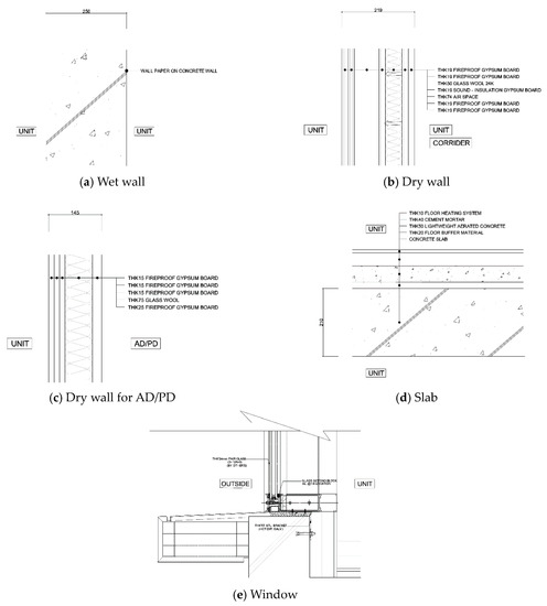
Figure 4.
Section view of each wall type.
Based on an analysis of the components of the envelope in a residential unit, the variables were grouped into variables related to the areas of envelope components and variables related to the connection lengths between different components. The area-related variables include the areas of the slabs, concrete wall, drywall, AD/PD drywall, window, entrance door, and louver connecting to the outdoor unit space. The connection-length-related variables include the connection lengths between a drywall and a drywall, a concrete wall and a concrete wall, and between a drywall and a concrete wall, and the connection lengths of the window, AD/PD wall, outdoor unit space louver, and entrance door. Table 3 lists the notation and description of the variables used. For example, Aslab is the sum of the slab area and ceiling area and lies within the range of 193–421 m2. Since all of the walls are constructed as concrete walls in Complex A, the values of AdryW and LdryWconc.W are 0. Additionally, in Type B-2, the outdoor unit space is installed at the exterior of the residential unit, so the values of Alouver and Llouver are 0.

Table 3.
Envelope element variables—predictor details.
4. Correlation Analysis
The previous section presented the process of identifying independent variables in the prediction model. However, it is also necessary to analyze the influence of each variable by investigating the relationship between the extracted independent variables and the ACH50 value, which will serve as the dependent variable. In this section, statistical correlation analysis is applied for this purpose.
4.1. Correlation Analysis between Area Variables and ACH50
The correlations between airtightness (as measured by ACH50) and the seven area variables (Aslab, Aconc.W, AdryW, Awindow, AadpdW, Alouver, and Adoor) were analyzed. To check for correlations, scatter diagrams were employed. By observing the scatter diagrams as shown in Figure 5, it can be seen that the slab area and window area exhibit the most linear relationships and are more relevant to airtightness than the other variables. The variable Aslab exhibits a negative relationship (Pearson correlation coefficient = −0.780), with an increase in area causing a decrease in ACH50, after which the window area (Pearson correlation coefficient = −0.453) exhibits a higher correlation compared to other variables. The correlation coefficients for the correlations between airtightness and the area variables are listed below in Table 4. The slab, window, and concrete wall variables are statistically significant at the 95% confidence level. It is deduced that these three variables are highly related with ACH50. The analysis of statistical correlations and correlation coefficients shows that the areas of the slab and the window have the highest correlations with airtightness and that the area of the concrete wall has the next highest correlation.
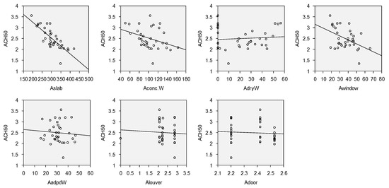
Figure 5.
Analysis result of scatter diagrams between seven areas (Aslab, Aconc.W, AdryW, Awindow, AadpdW, Alouver, and Adoor) variables and airtightness.

Table 4.
Statistical correlations and correlation coefficients (area variables).
4.2. Correlation Analysis between Connection Length Variables and ACH50
The correlations between airtightness (as measured by ACH50) and the seven connection length variables (LdryWdryW, Lconc.Wconc.W, LdryWconc.W, Lwindow, Ladpd, Llouver, and Ldoor) were analyzed. To check for correlations, scatter diagrams were employed. By observing the scatter diagrams in Figure 6, it can be seen that only the connection length corresponding to the perimeter length of the window exhibits a linear relationship and that other connection length variables do not exhibit correlations with airtightness. There is a negative relationship such that an increase in the connection length of the window causes a decrease in ACH50. Upon analyzing the correlation coefficients shown in Table 5, it can be seen that the variable of connection length of the window is highly related (95% confidence level) with ACH50. Thus, it is observed that, in a residential unit, only the connection length of the window has a correlation with airtightness.
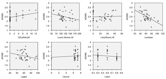
Figure 6.
Analysis result of scatter diagrams between seven connection length (LdryWdryW, Lconc.Wconc.W, LdryWconc.W, Lwindow, Ladpd, Llouver, and Ldoor) variables and airtightness.

Table 5.
Statistical correlations and correlation coefficients (connection length variables).
5. Prediction Model using Multiple Linear Regression Analysis
Multiple linear regression analysis, used as the main method in the prediction model, is capable of providing predictive results and also presenting the statistical significance of each variable on the predicted value. Multiple linear regression analysis was applied to the geometrical information of a target building (the area and connection lengths of the envelope) to predict the airtightness of a residential unit in an apartment building. The airtightness values of the 477 units obtained from measurements and data relating to the geometrical components of their envelopes were used as variables, which were applied to a sample regression model as shown below.
where is the dependent variable (ACH50); are the independent variables; is the constant value; are the regression coefficients; and is the error term that accounts for the discrepancy between the model and the observations. In the prediction model above, is a dependent variable, while the building parameters are independent variables. In this study, the independent variables were grouped into two types as discussed above, variables related to the areas and the connection lengths of envelope components. The area variables were set for the slab, concrete wall, drywall, AD/PD drywall, window, entrance door, and outdoor unit space louver. The connection length variables were set for the connections between a drywall and a drywall, a concrete wall and a concrete wall, and between a drywall and a concrete wall, and the connections of the window, AD/PD drywall, outdoor unit space louver, and entrance door. A prediction model was derived by way of multiple linear regression analysis, utilizing the IBM SPSS Statistics Version 21 statistics program [37].
The fitness of a prediction model based on a regression analysis is usually identified with the value of the adjusted R-squared. Additionally, the prediction accuracy representing the reliability of the proposed prediction model is verified by comparing the predicted values with the actual values in identical conditions. This study used two methods to verify the prediction accuracy of the models: the root-mean-square error (RMSE) and the mean absolute percentage error (MAPE). Equations (2) and (3) show how to calculate RMSE and MAPE.
where is the root mean square error, is the mean absolute percentage error, is the number of data, is the actual value, and is the forecast value.
5.1. Multiple Linear Regression Analysis Including All Variables for Area and Connection Length
The first step in achieving feasible prediction models based on multiple linear regression analysis is to establish a model using all variables, including seven variables focusing on area and seven variables focusing on connection length. Multiple regression analysis produces several prediction models for all variables, which were derived from Equations (4) to (6).
Table 6 shows the details of the prediction models using all variables. The analysis suggests a total of three feasible prediction models, as shown in Table 6. All variables selected in the models are statistically significant within a 95% confidence interval. More serious, however, are the values of the VIF (variance inflation factor) which have been used to indicate the degree of independence of the variables. Statistically, if the VIF value is greater than 10, the independence of the variable adopted is not confirmed, and this will not satisfy the fundamental assumptions of the regression models. The VIF values of the Lconc.Wconc.W and Aconc.W variables used in the third model are close to 10, which could indicate a serious problem caused by multicollinearity. All variables related to area and connection length were inputted, and the variables inputted and removed for each model as a result of the stepwise selection method are shown below in Table 7.

Table 6.
Coefficients of the models with all variables for area and connection length.

Table 7.
Inputted/removed variables in the models with all variables.
The results obtained by applying multiple linear regression analysis and analysis of variance (ANOVA) to the prediction models are summarized in Table 8 and Table 9, respectively. Results based on a stepwise method show that the third model is the most appropriate model, considering the adjusted R-squared value (representing the fitness of the predictive model) and the RMSE and MAPE (showing the degree of model verification). The adjusted R-squared, RMSE, and MAPE of the third model indicate that this is the best prediction model from the statistical point of view. In this case, the adjusted R-squared, RMSE, and MAPE of the final prediction model using all variables are 0.500, 0.32673, and 10.58107, respectively. The ANOVA analysis results in Table 9 indicate that all five prediction models are statistically significant within a 95% confidence interval, showing the significance probability of 0.000 (p-Value < 0.05).

Table 8.
Summary of the models with all variables for area and connection length.

Table 9.
ANOVA table of the models with all variables for area and connection length.
5.2. Multiple Linear Regression Analysis between Area Variables and ACH50
As a result of multiple linear regression analysis conducted between airtightness (as measured by ACH50) and the area of each component, a regression model was derived, as shown below in Equations (7) and (8).
Thus, the regression model trends such that an increase in the area of the slab leads to a decrease in the ACH50 value, while an increase in the area of the drywall leads to an increase in the ACH50 value. The resulting regression analysis coefficients shown in Table 10 show that the area of the slab has a large impact and the area of the drywall has the next largest impact, similar to the results of the correlation analysis. The standardized coefficients of the slab area and the drywall area were −0.801 and 0.180, respectively. The variance inflation factors (VIFs) are below 10 for both variables, and it is therefore deemed that there is no multicollinearity. The regression analysis conducted on ACH50 and the area variables employed a stepwise selection method. All seven variables related to area were inputted, and the variables inputted and removed for each model as a result of the stepwise selection method are shown below in Table 11.

Table 10.
Coefficients of the models with variables for area.

Table 11.
Inputted/removed variables in the models with variables for area.
A summary of the multiple linear regression analysis results is provided in Table 12. The coefficient of determination (R-squared value), which represents suitability, of the prediction model with seven inputted variables inputted is 0.641, meaning it has an explanatory power of about 64%. The adjusted R-squared value is 0.619. The values of RMSE and MAPE for model verification are 0.30418 and 9.94311, respectively. The Durbin–Watson value, which represents autocorrelation between the variables, is found to be 1.743, and it is deemed that the regression analysis method employed as the analysis method for this model is appropriate. In Table 13, which presents a variance analysis of the results of the multiple linear regression analysis, the significance probability is 0.000 (p < 0.05), and it is therefore determined that the prediction model is statistically significant.

Table 12.
Summary of the models with variables for area.

Table 13.
ANOVA table of the models with variables for area.
5.3. Multiple Linear Regression Analysis between Connection Length Variables and ACH50
As a result of multiple linear regression analysis conducted between airtightness (as measured by ACH50) and the connection length of each component, a regression model was derived, as shown below in Equations (9) to (12).
Equation (12) shows a model in which increases in the connection lengths of the window and the AD/PD drywall lead to a decrease in the ACH50 value, while an increase in the connection length of the outdoor unit space louver leads to an increase in the ACH50 value. The resulting coefficients of the regression analysis are summarized below in Table 14. Similar to the results of the correlation analysis above, it is found that the connection length of the window has the largest impact.

Table 14.
Coefficients of the models with variables for connection length.
The standardized coefficients of the variables are shown to be −0.544, 0.258, 0.308, and −0.216 for the window, drywall and drywall, outdoor unit space louver, and AD/PD drywall connection lengths, respectively. The variance inflation factors (VIFs) are below 10 for all variables, and it is therefore deemed that there is no multicollinearity between the independent variables. Thus, a major assumption of the prediction model, that there is independence between the independent variables, is ascertained.
The regression analysis for the connection length variables also employed a stepwise selection method, similar to the case of the area variables, and the variables inputted and removed for each model are shown below in Table 15.

Table 15.
Inputted/removed variables in the models with variables for connection length.
Looking at the summary for the variables representing connection lengths between components, the coefficient of determination (R-squared value), which represents suitability, is 0.451, meaning that it has an explanatory power of about 45% in regard to airtightness (Table 16). The adjusted R-squared value is relatively low (0.378). The values of RMSE and MAPE for model verification are 0.39301 and 13.23147, respectively. The Durbin–Watson value, which represents autocorrelation between the variables, is found to have a reasonable value of 1.560. Thus, it is deemed that the regression analysis method applied for implementing the model is appropriate. As seen Table 17, which shows variance analysis results, the significance probability is shown to be 0.001 (P < 0.05), and it is therefore determined that the present model is statistically significant.

Table 16.
Summary of the models with variables for connection length.

Table 17.
ANOVA table of the models with variables for connection length.
5.4. Summary
This study presents the proposed prediction models using the variables that affect the ACH value. For more precise analysis, this study identifies all the variables that may affect ACH50 values, and then separates these variables into area and connection length to establish more reliable prediction models. Table 18 lists the main results of the analysis of the best models for each of the following cases: considering the impact of all variables on airtightness, considering the impact of variables pertaining to the areas of individual components on airtightness, and considering the impact of variables pertaining to connection lengths between components on airtightness. The results of the multiple linear regression analysis show that, while all three models are satisfactory in terms of the Durbin–Watson value, VIF, and significance probability, the model with all variables and the model with variables for connection length have relatively low adjusted R-squared explanatory coefficient (representing the suitability of the prediction models) values of 0.500 and 0.378, respectively. These may be compared to the adjusted R-squared of the model with variables for area, which presents a value of 0.619 (or an explanatory power of about 61.9%). The RMSE and MAPE values for the degree of model verification are also 0.30418 and 9.94311, respectively, which are relatively low compared to the two models with all variables and variables for connection length. The multicollinearity of the model with all variables is concerning since the variables for area and those for connection length are strongly related to each other. This limits the ability to satisfy the condition of independence between the variables when all these variables are used to construct single prediction model. This is also reflected in the VIF values, which are close to 10 (e.g., 8.924 and 9.182) for many of variables used in this model. As such, Equation (8), the prediction model based on area variables, is determined to be more suitable as an airtightness prediction model compared to the prediction model based on connection length variables. In Equation (8), larger areas for the floor and ceiling lead to lower ACH50 values, while larger areas for the drywall lead to higher ACH50 values. Although leakage and infiltration may actually occur through the removed variables, i.e., variables related to the concrete wall, window, AD/PD wall, outdoor unit space louver, and entrance door, it is deemed that they are removed from the predictor variables because the areas of these components are distributed within a particular range or because they do not display suitable correlations with airtightness. The regression model derived in this study is a statistically derived model for predicting airtightness and does not necessarily apply to the predicting of airtightness in every apartment building. It is deemed, however, that the model can serve as a meaningful reference when predicting airtightness in apartment buildings where it is not possible to actually measure airtightness.

Table 18.
Summary of the results of multiple linear regression analysis for each variable group.
6. Conclusions
This study uses multiple linear regression analysis to derive a model equation for predicting the airtightness of reinforced concrete apartment buildings, which are frequently constructed as high-rises in Asian countries. Based on airtightness data measured in the form of ACH50 values from 477 residential units, connection length variables and area variables pertaining to the components of the envelope were used to derive a prediction model equation for each variable type.
Upon reviewing the correlations for each of the variables, it was determined that the slab area (floor and ceiling area) has the highest correlation from among the area variables and that the window perimeter length has the highest correlation from among the connection length variables. It is determined that this is because of the high importance attached to the area occupied by a material with a different airtightness level, considering that the residence units mostly have similar forms. The R-squared value and adjusted R-squared value for the area variable model were calculated to be 0.641 and 0.619, respectively, higher than the values for the model that includes all variables and those for the models that incorporate connection length variables. Between the two groups of variables representing the information of the envelope, the ‘area prediction model’ is found to have a higher level of prediction reliability compared to the ‘connection length prediction model’. It is found that larger areas for the floor and ceiling of the residential unit would result in lower ACH50 values, while larger areas for the drywall would result in less desirable airtightness. To improve airtightness, it would be necessary to employ airtight construction and management techniques at the slab portions of the floor and ceiling, drywalls, and connection portions corresponding to the perimeter of the windows.
The airtightness prediction model of the present study is part of explanatory research efforts that highlight the possibility of using the geometric information of a building envelope in predicting airtightness and is not a universal model that can be applied to buildings of all usages or forms. That is, the main purpose of the study is to discover which factors are statistically meaningful from among the geometrical information (area elements and connection length elements) of the envelope that has direct relevance to the airtightness of the building. Besides the geometrical information of the envelope, nonstandardized factors such as construction quality can also impact airtightness and may serve as subjects for future research. In spite of the large amount of measured data used, there is a limit to applying the prediction model equation presented in this study to the estimation of airtightness in all apartment buildings, since the properties of the buildings may differ in other countries. However, the study is meaningful in that it highlights the possibility of using the geometrical components of the envelope for predicting airtightness in residential units of apartment buildings that are mass-produced in similar forms using reinforced concrete techniques. The airtightness prediction model can be utilized for estimating airtightness data needed for conducting energy performance evaluations for residential units of apartment buildings with lower costs in a reduced time. In addition, it can be used to check which portions may require supplementation if improvements in airtightness are desired.
Author Contributions
Conceptualization, J.-H.J.; Data collection, K.-H.J, and H.-K.S.; Data analysis and Model configuration, S.H. and K.-H.J.; Writing-original draft, K.-H.J.; Writing-review & editing, S.H. and J.-H.J.; All authors have involved in reading and agreeing to the published version of the manuscript.
Funding
This work was supported by an Inha University Research Grant.
Conflicts of Interest
The authors declare no conflict of interest
References
- ISO 13790. Energy Performance of Buildings—Calculation of Energy Use for Space Heating and Cooling; ISO: London, UK, 2008. [Google Scholar]
- François, R.C.; Peter, W. Building Airtightness: A Critical Review of Testing, Reporting and Quality Schemes in 10 Countries. TightVent Report no 4. 2012. Available online: https://www.aivc.org/sites/default/files/members_area/medias/pdf/Technotes/TN67_Building%20airtightness.pdf (accessed on 1 June 2016).
- Kaewunruen, S.; Sresakoolchai, J.; Kerinnonta, L. Potential reconstruction design of an existing townhouse in Washington DC for approaching net zero energy building goal. Sustainability 2019, 11, 6631. [Google Scholar] [CrossRef]
- Kaewunruen, S.; Rungskunroch, P.; Welsh, J. A digital-twin evaluation of Net Zero Energy Building for existing buildings. Sustainability 2018, 11, 159. [Google Scholar] [CrossRef]
- Available online: http://passiv.de/ (accessed on 1 June 2016).
- Sherman, M.H.; Chan, R. Building Air Tightness: Research and Practice; LBNL Report 53356; Lawrence Berkeley National Lab.: Berkeley, CA, USA, 2003. [Google Scholar]
- ASHRAE. ASHRAE Handbook Fundamentals, American Society of Heating, Refrigerating and Air conditioning Engineers; ASHRAE Handbook: Atlanta, GA, USA, 2017. [Google Scholar]
- Yoshino, H. The current of air-tightness and ventilation system in Houses of Japan. In Proceedings of the 29th AIVC conference, Kyoto, Japan, 14–16 October 2008; pp. 341–347. [Google Scholar]
- Jokisalo, J.; Kurnitski, J.; Korpi, M.; Kalamees, T.; Vinha, J. Building leakage, infiltration, and energy performance analyses for Finnish detached houses. Build. Environ. 2009, 44, 377–387. [Google Scholar] [CrossRef]
- Chan, W.R.; Joh, J.; Sherman, M.H. Analysis of air leakage measurements of US house. Energy Build. 2013, 66, 616–625. [Google Scholar] [CrossRef]
- Pan, W. Relationships between air-tightness and its influencing factors of post-2006 new-build dwellings in the UK. Build. Environ. 2010, 45, 2387–2399. [Google Scholar] [CrossRef]
- Shin, H.-K.; Jo, J.-H. Characteristics and Leakage Distribution of Dwellings in High-rise Residential Buildings in Korea. J. Asian Archit. Build. Eng. 2013, 12, 87–92. [Google Scholar] [CrossRef]
- Sfakianaki, A.; Pavlou, K.; Santamouris, M.; Livada, I.; Assimakopoulos, M.-N.; Mantas, P.; Christakopoulos, A. Air tightness measurements of residential houses in Athens, Greece. Build. Environ. 2008, 43, 398–405. [Google Scholar] [CrossRef]
- Iordache, V.; Nastase, I.; Damian, A.; Colda, I. Average permeability measurements for an individual dwelling in Romania. Build. Environ. 2011, 46, 1115–1124. [Google Scholar] [CrossRef]
- Relander, T.-O.; Holøs, S.; Thue, J.V. Airtightness estimation—A state of the art review and an en route upper limit evaluation principle to increase the chances that wood-frame houses with a vapour- and wind-barrier comply with the airtightness requirements. Energy Build. 2012, 54, 444–452. [Google Scholar] [CrossRef]
- Kondratyev, K.Y.; Varotsos, C. Atmospheric greenhouse effect in the context of global climate change. Nuovo Cim. C 1995, 18, 123–151. [Google Scholar] [CrossRef]
- Pietrzyk, K.; Hagentoft, C.-E. Probabilistic analysis of air infiltration in low-rise buildings. Build. Environ. 2008, 43, 537–549. [Google Scholar] [CrossRef]
- Fernández-Agüera, J.; Domínguez-Amarillo, S.; Sendra, J.J.; Suárez, R. An approach to modelling envelope airtightness in multi-family social housing in Mediterranean Europe based on the situation in Spain. Energy Build. 2016, 128, 236–253. [Google Scholar] [CrossRef]
- Krstić, H.; Koški, Ž.; Otković, I.I.; Španić, M. Application of neural networks in predicting airtightness of residential units. Energy Build. 2014, 84, 160–168. [Google Scholar] [CrossRef]
- Krstić, H.; Otković, I.I.; Kosiński, P.; Wójcik, R. Validation of neural network model for predicting airtightness of residential and non-residential units in Poland. Energy Build. 2016, 133, 423–432. [Google Scholar] [CrossRef]
- Sherman, M.H. Air Leakage of US Homes: Model Prediction; ASHRAE: Atlanta, GA, USA, 2007. [Google Scholar]
- Prignon, M.; Moeseke, G.V. Factors influencing airtightness and airtightness predictive models: A literature review. Energy Build. 2017, 146, 87–97. [Google Scholar] [CrossRef]
- Fernández-Agüera, J.; Domínguez-Amarillo, S.; Sendra, J.J.; Suarez, R. Predictive models for airtightness in social housing in a Mediterranean region. Sustain. Cities Soc. 2019, 51, 101695. [Google Scholar] [CrossRef]
- Montoya, M.I.; Pastor, E.; Carrié, F.R.; Guyot, G.; Planas, E. Air leakage in Catalan dwellings: Developing an airtightness model and leakage airflow predictions. Build. Environ. 2010, 45, 1458–1469. [Google Scholar] [CrossRef]
- Berge, A. Analysis of Methods to Calculate Air Infiltration for Use in Energy Calculations; Chalmers University of Technology: Gothenburg, Sweden, 2011. [Google Scholar]
- Iordache, V.; Catalina, T. Acoustic approach for building air permeability estimation. Build. Environ. 2012, 57, 18–27. [Google Scholar] [CrossRef]
- Hayati, A.; Mattsson, M.; Sandberg, M. Evaluation of the LBL and AIM-2 air infiltration models on large single zones: Three historical churches. Build. Environ. 2014, 81, 365–379. [Google Scholar] [CrossRef]
- Feustel, H. COMIS-an international multizone air-flow and contaminant transport model. Energy Build. 1999, 30, 3–18. [Google Scholar] [CrossRef]
- Dols, W.S.; Polidoro, B.J. CONTAM User Guide and Program Documentation Version 3.2. Nist Tech. Note 2015, 1887. [Google Scholar] [CrossRef]
- Han, G.; Srebric, J.; Enache-Pommer, E. Different modeling strategies of infiltration rates for an office building to improve accuracy of building energy simulations. Energy Build. 2015, 86, 288–295. [Google Scholar] [CrossRef]
- Axley, J. Multizone Airflow Modeling in Buildings: History and Theory. Hvacr Res. 2007, 13, 907–928. [Google Scholar] [CrossRef]
- Feustel, H.E.; Dieris, J. A survey of airflow models for multizone structures. Energy Build. 1992, 18, 79–100. [Google Scholar] [CrossRef]
- Roulet, C.-A.; Fürbringer, J.-M.; Cretton, P. The influence of the user on the results of multizone air flow simulations with COMIS. Energy Build. 1999, 30, 73–86. [Google Scholar] [CrossRef]
- Feijó-Muñoz, J.; Poza-Casado, I.; González-Lezcano, R.A.; Pardal, C.; Echarri, V.; Assiego De Larriva, R.; Fernández-Agüera, J.; Dios-Viéitez, M.J.; Del Campo-Díaz, V.J.; Montesdeoca Calderín, M.; et al. Methodology for the Study of the Envelope Airtightness of Residential Buildings in Spain: A Case Study. Energies 2018, 11, 704. [Google Scholar] [CrossRef]
- Wallace, L.A.; Emmerich, S.J.; Howard-reed, C. Continuous measurements of air change rates in an occupied house for 1 year: The effect of temperature, wind, fans, and windows. J. Expo. Anal. Environ. Epidemiol. 2002, 12, 296–306. [Google Scholar] [CrossRef]
- ASTM E779. Standard Test Method for Determining Air Leakage Rate by Fan Pressurization; ASTM: West Conshohocken, PA, USA, 2010. [Google Scholar]
- IBM Corp. Released, IBM SPSS Statistics for Windows; Version 21.0; IBM Corp.: Armonk, NY, USA, 2012. [Google Scholar]
© 2020 by the authors. Licensee MDPI, Basel, Switzerland. This article is an open access article distributed under the terms and conditions of the Creative Commons Attribution (CC BY) license (http://creativecommons.org/licenses/by/4.0/).
