Near Real-Time Global Solar Radiation Forecasting at Multiple Time-Step Horizons Using the Long Short-Term Memory Network

Abstract

This paper aims to develop the long short-term memory (LSTM) network modelling strategy based on deep learning principles, tailored for the very short-term, near-real-time global solar radiation (GSR) forecasting. To build the prescribed LSTM model, the partial autocorrelation function is applied to the high resolution, 1 min scaled solar radiation dataset that generates statistically significant lagged predictor variables describing the antecedent behaviour of GSR. The LSTM algorithm is adopted to capture the short- and the long-term dependencies within the GSR data series patterns to accurately predict the future GSR at 1, 5, 10, 15, and 30 min forecasting horizons. This objective model is benchmarked at a solar energy resource rich study site (Bac-Ninh, Vietnam) against the competing counterpart methods employing other deep learning, a statistical model, a single hidden layer and a machine learning-based model. The LSTM model generates satisfactory predictions at multiple-time step horizons, achieving a correlation coefficient exceeding 0.90, outperforming all of the counterparts. In accordance with robust statistical metrics and visual analysis of all tested data, the study ascertains the practicality of the proposed LSTM approach to generate reliable GSR forecasts. The Diebold–Mariano statistic test also shows LSTM outperforms the counterparts in most cases. The study confirms the practical utility of LSTM in renewable energy studies, and broadly in energy-monitoring devices tailored for other energy variables (e.g., hydro and wind energy).

1. Introduction

Conventional energies (e.g., fossil fuel) have been a primary energy resource for many decades [1,2,3]; however, these resources are being replaced gradually by various renewable resources as a pivotal solution that aims to meet the future energy crisis caused by their depleting nature and the environmental damage caused by greenhouse gas emissions through the burning of carbon-positive fuel [4,5]. Following the global trends in energy exploration [6,7,8] and the recommendations of the United Nations Sustainable Development Goal that advocates a dire need for cleaner, affordable and accessible energy in all nations and regions. Thus, Vietnam has recently commenced capacity development for solar energy resources. With its geographical location close to the solar energy belt, Vietnam can harvest this energy from freely available sunlight, theoretically, providing 60–100 GWh·year⁻¹ of solar concentrated power and 0.8–1.2 GWh·year⁻¹ as photovoltaic power [9]. These figures advocate a continuous growth of solar energy which will meet the increasing consumer power demand. As such, it is important to develop modern technologies for energy management systems that purposely support real-time energy integration in a power grid or a distribution system [10]. An accurate near-real-time forecasting tool, especially tailored for solar energy management and proportional dispatching to and from a grid system is therefore a scientific contrivance for the update of solar energy into a real grid system [11].

Solar energy forecasting is typically based on consumer usage to provide greater stability and energy regulation, reverse management and dispatching, scheduling and unit commitments [11]. For each of the consumer’s usages, the forecasting timescales can vary from being a long-term forecast (e.g., a monthly forecast) [12] to a mid-term forecast (e.g., a day-ahead forecast) [13,14] and to a short-term forecast (e.g., an hour-ahead) period [15,16]. However, studies on a very short-term or near-real-time forecast are relatively scarce, thus, the present research work aims to fulfil this need.

There are many approaches in solar radiation forecasting, divided roughly into data-driven (or artificial intelligence) and physical (atmospheric dynamic) models [17]. Many existing studies, however, reveal limitations in forecasting techniques (e.g., computational resources to calibrate a huge volume of data, thus encountering unexpected errors) and challenges arising from complexity of predictor variables (e.g., intermittent and chaotic properties of consumer demands, meteorological and geographical data) [11,18]. To overcome these issues, the present research work is focused on developing a new modelling strategy for near-real-time solar radiation forecasting by implementing the latest deep learning techniques.

The construction of a solar radiation-forecasting model in general and the global solar radiation (GSR) model, in particular, have been intensively explored. With the recent advances of computational data science, machine learning-based forecasting models typically provide distinct advantages over physical models [17,19,20] and time-series models [21,22,23,24,25,26,27,28,29,30,31,32,33,34,35]. Models based on machine learning and neural networks have evolved over recent decades. However, common weaknesses have been reported, such as those causing bias when extending data volume, and over-fitting [11]. Deep learning techniques, the latest advancement of machine learning, can solve the above issues but have not been fully explored. On the other hand, solar forecasting is relatively new in Vietnam, although there were previous studies of solar radiation [36,37,38] and solar potential mapping [39] in recent decades. Studies implementing machine learning methods for solar forecasting can be found in other Asian countries [40,41,42,43]. However, the application of these techniques has not been performed in the context of Vietnam, although a recent study with a similar approach was undertaken in Australia [44]. Nonetheless, to the best of the author’s knowledge, the present study is the first exploring the predictive power of a deep learning method—the long short-term memory (LSTM) network model for minute-ahead solar energy forecasting, particularly in the context of Vietnam where the prospect for solar powered energy systems is relatively high.

This study adopts long short-term memory (LSTM) networks, a branch of deep neural networks, which has shown an excellent ability to handle predictive issues and has been extensively employed in image recognition, automatic speech recognition and natural language processing [45,46,47,48,49,50,51,52]. LSTM is believed to overcome limitations of conventional data-driven models in capturing short- and long-term dependency between a target (e.g., future solar radiation) and corresponding historical variables and big data issues. In addition, due to its ability of removing abundant information to resolve vanishing gradient issues, LSTM is appropriate to represent the learning data over different temporal domains [17]. Hence, LSTM has been studied in solar forecasting during the past five years [15,17,44,53,54,55,56,57,58,59,60,61,62,63]. For instance, the first study regarding LSTM [64] demonstrated its forecasting skills for one-day ahead utilizing remote-sensing data under various topographical conditions with the best root mean square error (RMSE) ~24% and mean absolute error (MAE) ~17%. In [15,65], LSTM performed well for one-day-ahead forecasting under multiple seasonal and weather conditions. Generally, although forecasting methods show their predictive skills in a different context, optimizing the forecasting methods has still been an important problem of interest. Similarly, developing an optimal LSTM model in terms of solar energy forecasting is also under consideration. Most recent papers have focused on data pre-processing techniques to optimize predictive results [59,60,66,67]; hence, there is a lack of intensive papers relating to optimizing the LSTM technique itself. Moreover, a huge dataset volume was discussed in the context of traditional time-series methods which pointed out that performance efficiency decreased against the increase of data volume. Thus, the present work aims to extensively explore optimization and performance assessment of the LSTM forecasting technique in the near-real-time case by also considering multiple performance metrics (i.e., relative prediction errors, including Willmott’s index, the Nash–Sutcliff index, and the Legates and McCabe index) adopted for multiple forecast horizons ranging from 1 min to ½ h periods.

In terms of the model performance evaluation, despite higher levels of model assessment skill in the error measurement approaches compared with the correlation coefficient (r) which represents the relationship between observed and predicted values [68], it is not totally sensible when applying RMSE and MAE alone [44,69], especially in deep learning method evaluation. Therefore, it is reasonable to apply multiple metrics in model performance evaluation to avoid their specific weaknesses [70]. For this reason, applying multiple evaluation metrics to assess the predictive performance of the LSTM method in near-real-time forecasts is a novelty in this paper.

Moreover, due to geographical location and weather condition, in some circumstances (e.g., Vietnam), it is difficult and costly to obtain such meteorological variables in a near-real-time horizon (i.e., minute interval). To address this issue, the present work will employ historical global solar radiation (GSR) time-series, data which is hardly seen in the literature.

Since the model’s accuracy is expected to decrease over the passage of time, the timescale of the forecasts encompasses the next minute of the GSR data in advance, to verify the persistence skill of the LSTM model. Therefore, to address the gaps in knowledge and also to advocate the need for a sustainable real-time energy management, the novelty of this paper is to firstly develop a near-real-time solar forecasting based on the integration of the LSTM algorithm. The paper also aims to emulate the LSTM model at multiple forecast horizons (i.e., 1, 5, 10, 15, 30 min) to ensure it is validated over a much longer period.

To perform this, a time series of the GSR data measured at the minute interval at a selected location (Bac-Ninh, Vietnam) is obtained. To demonstrate the advantages of the LSTM model in terms of near-real-time solar forecasting, this paper also compares LSTM performances against those of the traditional forecasting method, autoregressive integrated moving average (ARIMA), and the well-known machine learning methods of multilayer perceptron (MLP) network, support vector regression (SVR), and a deep learning method, deep neural network (DNN), in GSR near-real-time solar forecasting. As a representative of traditional forecast modelling, ARIMA and SVR are chosen for the modelling due to the non-stationary properties of the collected data [71]. Meanwhile, the MLP and DNN models are representative of neural network algorithms, which have been widely employed in recent decades [72,73]. To explore the predictive skill of the proposed method, the minute interval data is evaluated at multiple time horizons: 1 min (1 M), 5 min (5 M), 10 min (10 M), 15 min (15 M) and 30 min (30 M) forecast.

The main contributions of this study are as follows.

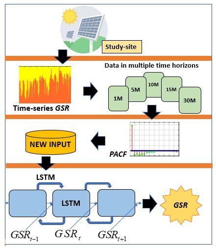
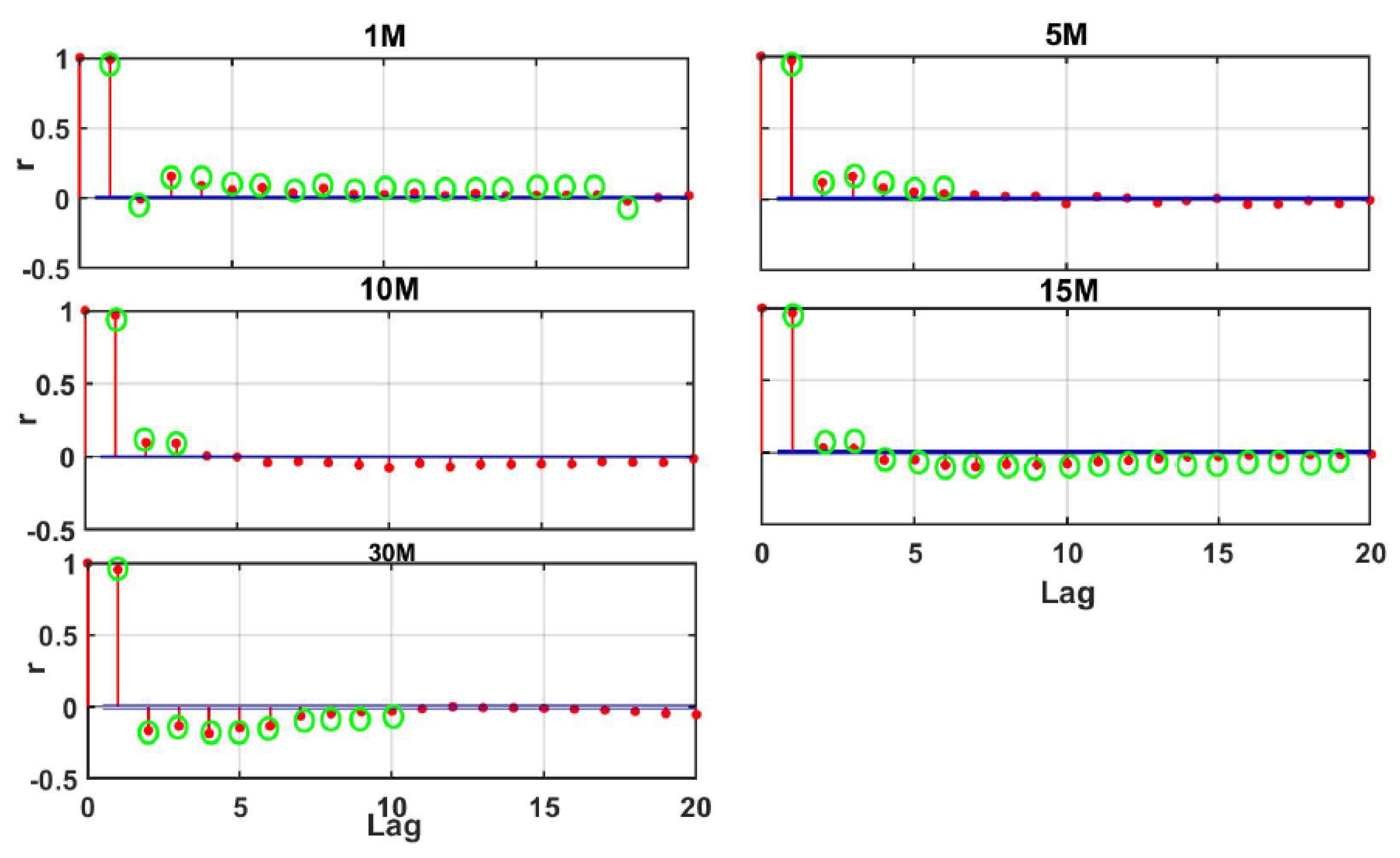
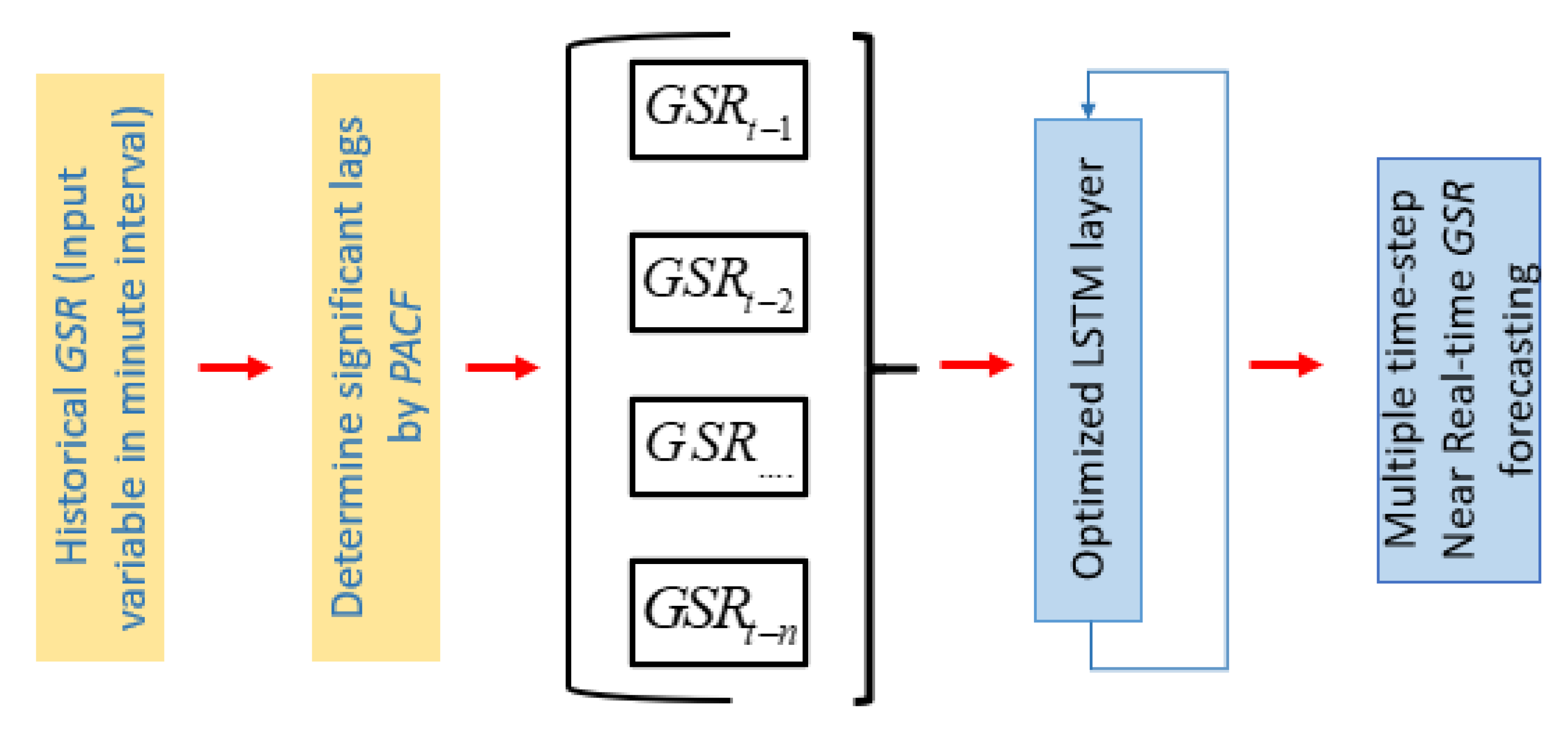
• Development and optimization of a near-real-time GSR forecasting method by implementing the LSTM algorithm for 1 min using lagged combinations of the aggregated GSR data as the predictor variables.
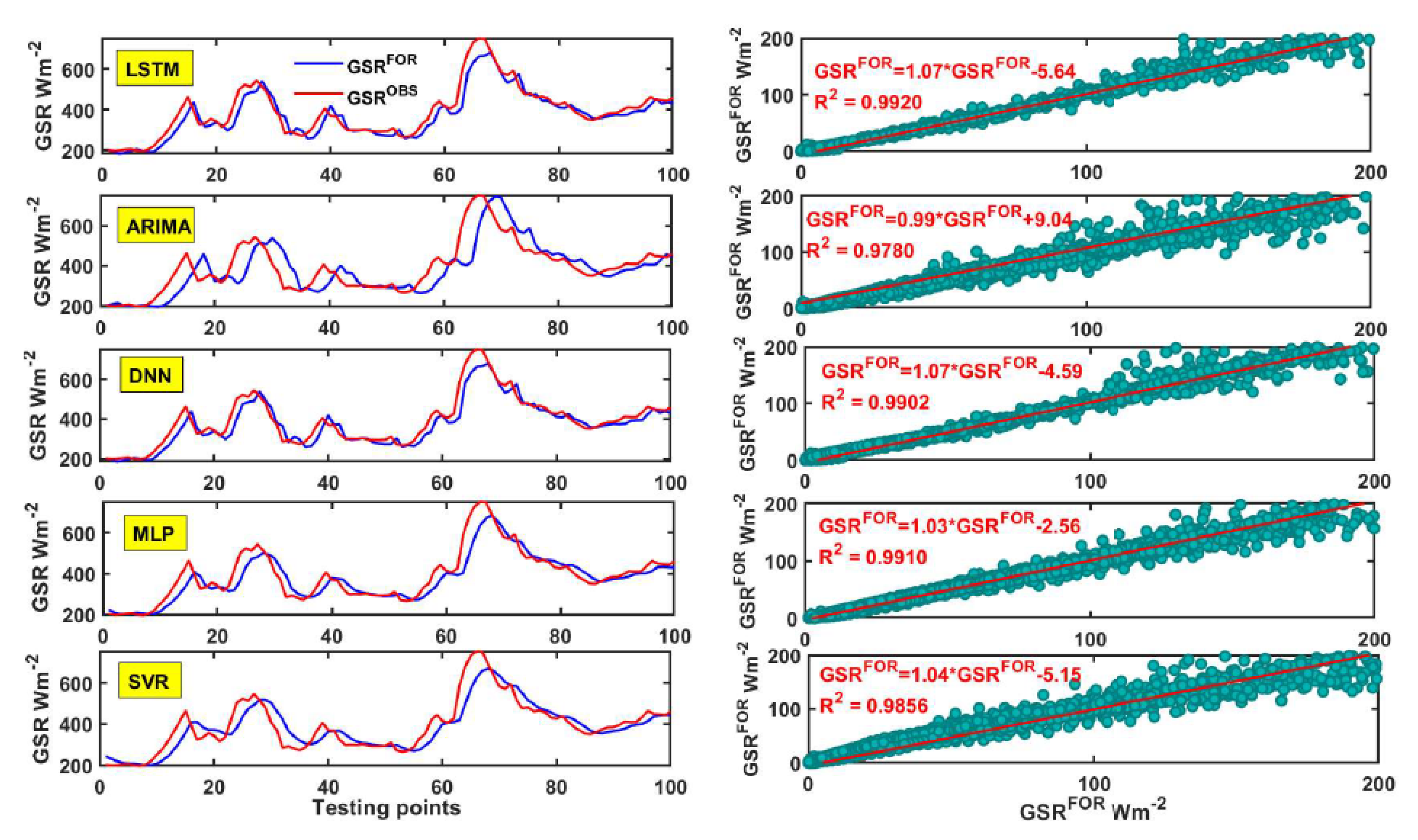
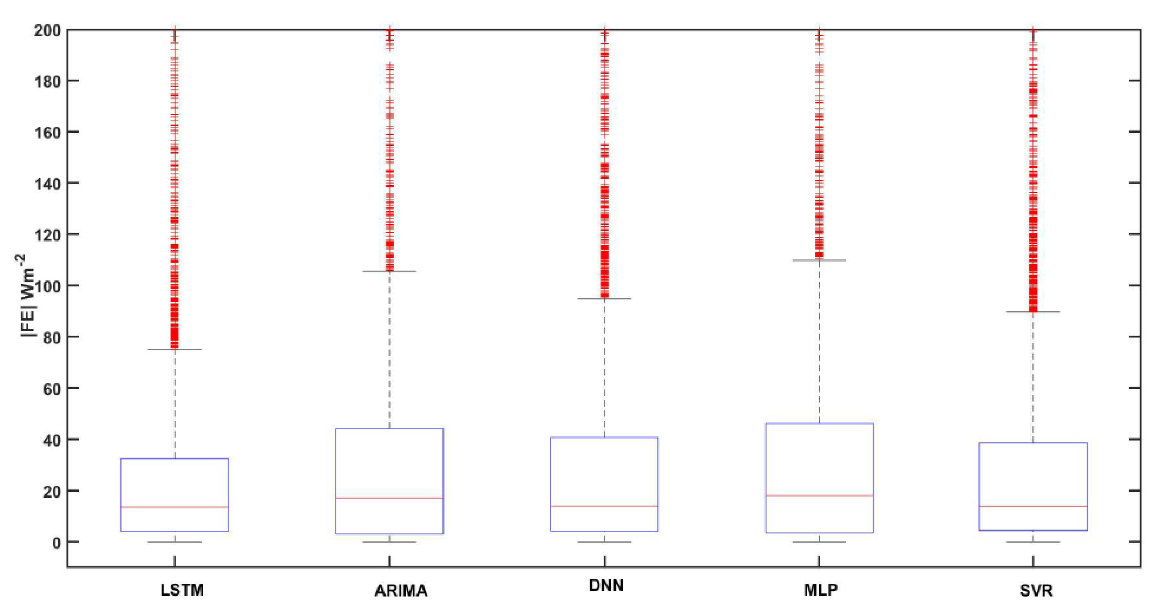
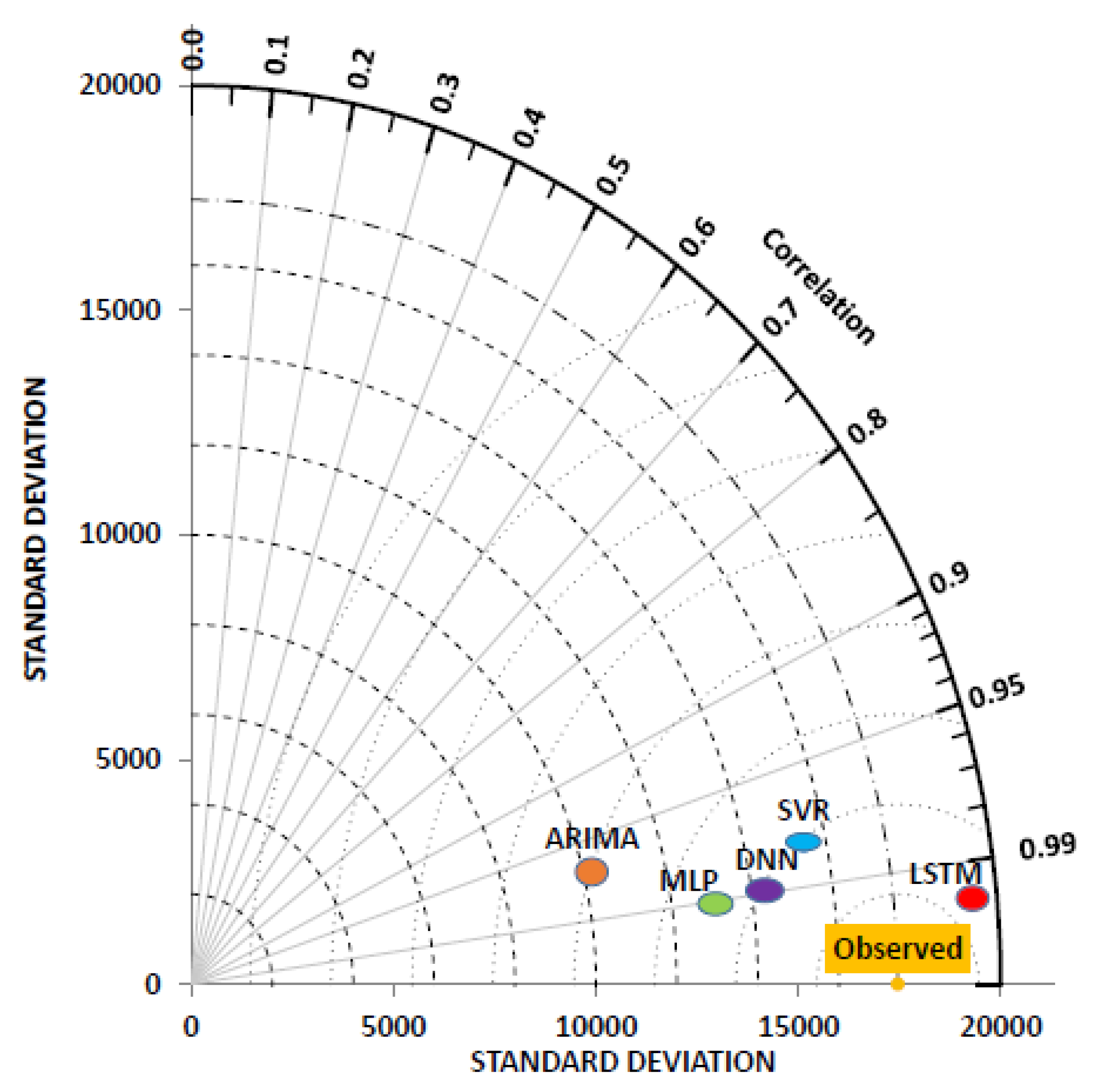
• Evaluation of the performance of the proposed model against benchmarked models (DNN, MLP, ARIMA, SVR) by a range of model evaluation metrics.
• Implementation of the proposed models for multi-minute ahead (e.g., 5 M, 10 M, 15 M, 30 M) and evaluation of the performance of LSTM over multiple forecast horizons.

To reach these objectives, this paper is organized as follows: Section 2 reviews previous literature. Section 3 presents a theoretical overview of the objective models. In Section 4, the dataset considered is introduced and explained, detailing model tuning and benchmark algorithms. Section 5 presents model performance metrics. A discussion of empirical results is available in Section 6 before the paper concludes in Section 7.

2. Related Work

In terms of solar irradiance forecasting, there is no one-fits-all modelling approach; in particular, the forecast horizon determines the suitability of alternative models (e.g., to support decision-making in operational management). Previous research has studied short-term models which forecast solar irradiance from 5 min to a few hours ahead. The focus of this paper is minute ahead forecasting (e.g., 1 min, 5 min, 10 min, 15 min and 30 min). A minute horizon is established in the literature and meaningful from an economic perspective since a rise in accuracy of solar energy forecasts may facilitate major cost savings [74]. The main purpose of minute-ahead forecasts is to maintain operational security [11].

In the following, previous studies with comparable forecast horizons from the past decade are discussed. Specifically, a review of solar irradiance forecasts using machine learning algorithms with forecast horizon of 30 min and below are given. The review [75,76,77] is based on a comprehensive study of several solar energy forecasting methods. A design of solar irradiance forecasts offers several research views and these complicate cross-study comparisons. Although studies often employ a specific spatio-temporal data in a unique context of weather characteristics, there is no guarantee that a method can be successful in all places and with all different time horizons. To depict a review of minute solar energy forecasting, the following table classifies and summarizes the previous related studies in terms of forecast horizon, corresponding data, and the employed forecasting methods.

As shown in

Table 1. Prior studies of near-real-time solar irradiance forecasting.

Study	Data Source	Time Resolution	Forecast Horizon	The Number of Data Points		Method
				Training Set	Testing Set	Proposed Method	Benchmark
[78]	GSR	5 min	5 min	24,260	8640	BPNN	Fuzzy Logic-BPNN
[79]	GSR	10 min	10 min	52,560	52,560	ELM	Persistent, BELM
[80]	TSI	1 min	15 min	68,833	8075	CNN	N/A
[81]	GSR	1 min	10 min	N/A	N/A	MLP	RBF
[82]	TSI	10 min	20 min	38,371	33,644	ARIMA	RW, MA, ES
[83]	GSR	15 min	15 min	21,170	1798	ANN	ANN, MLP, NARX
[84]	GSR	15 min	15 min	35,040	35,040	ARIMA	Persistence
[46]	TSI, GSR	1 min	5, 10, 15, 20 min	2016	864	CNN	Persistence
[58]	GSR	7.5 min	7.5, 15, 30, 60	201, 480	67, 160	LSTM	ARIMAX, MLP, Persistence

, several methods have been applied to different data sets with different spatio-temporal scales and time resolution, ranging from 1 to 7.5 min resolution. In addition, several forecast horizons have been tested, from a minute timescale to few-minutes-ahead forecasting. Moreover, Table 1 reveals few studies involving an evaluation of models across several forecast horizons and in a big data context. Except for [58], the authors devise a model for multiple forecast horizon with training sets greater than 100,000 points.

In terms of forecasting technique, these studies show that machine learning (ML) has good potential in very short-term solar energy forecasting. However, a limitation of ML algorithms is the insufficient learning models for high dimensional datasets [85], which directly influences the precision and accuracy of forecasting model by over-fitting and extrapolation [86]. By considering that the GSR time series often have long-term and short-term dependency in the low-frequency approximate parts, the long short-term memory (LSTM) network, a special type of recurrent neural network (RNN), is employed to predict the decomposed low-frequency sub-layer in this study.

Multiple conclusions emerge from Table 1. Firstly, the potential of LSTM has not been fully explored, especially in analysing high dimensional data at 1 min intervals. The similar conclusion can be found in [11]. Secondly, no study considers the efficiency of forecasting models for more than one forecast horizon. This might be due to the shortage of data in real time horizons. Finally, no study considers the ability of LSTM in dealing with data efficiency (e.g., data volume). Therefore, a restriction of prior studies is that they solely explain the GSR behaviour and forecasting efficiency in a specific context.

In this paper, the aim is to overcome these issues. Firstly, the forecasting ability across multiple forecast horizons through employing GSR accelerated from 1 min interval data for each horizon is demonstrated. This technique can resolve the shortage of available datasets, which facilitates a broader demonstration of the forecasting model efficiency across multiple forecast horizons. In addition, the bias toward data efficiency through employing different partition proportions in training and testing sets is addressed. An appropriate data proportion in forecasting models is thus carefully chosen. Finally, a high number of data points (over 100,000) is used for validation to test model efficiency in terms of big data.

As the objective technique in this study, LSTM is employed to prove its potential in real-time solar radiation forecasting, as well as dealing with high dimensional real-time GSR. As shown in Table 1, this approach has not yet been fully explored and previous studies on LSTM-based solar energy forecasting faced a risk of over-tuning [87]. Overcoming the limitation of the available dataset and facilitating multiple forecast horizons, the approach implemented in this study allows the mitigation of this risk using appropriate hyperparameter testing to optimize the LSTM model. With respect to benchmark methods, another deep learning technique (i.e., DNN), two machine learning techniques (i.e., MLP, SVR) and a statistical technique (i.e., ARIMA) are developed for comparison.

3. Theoretical Overview

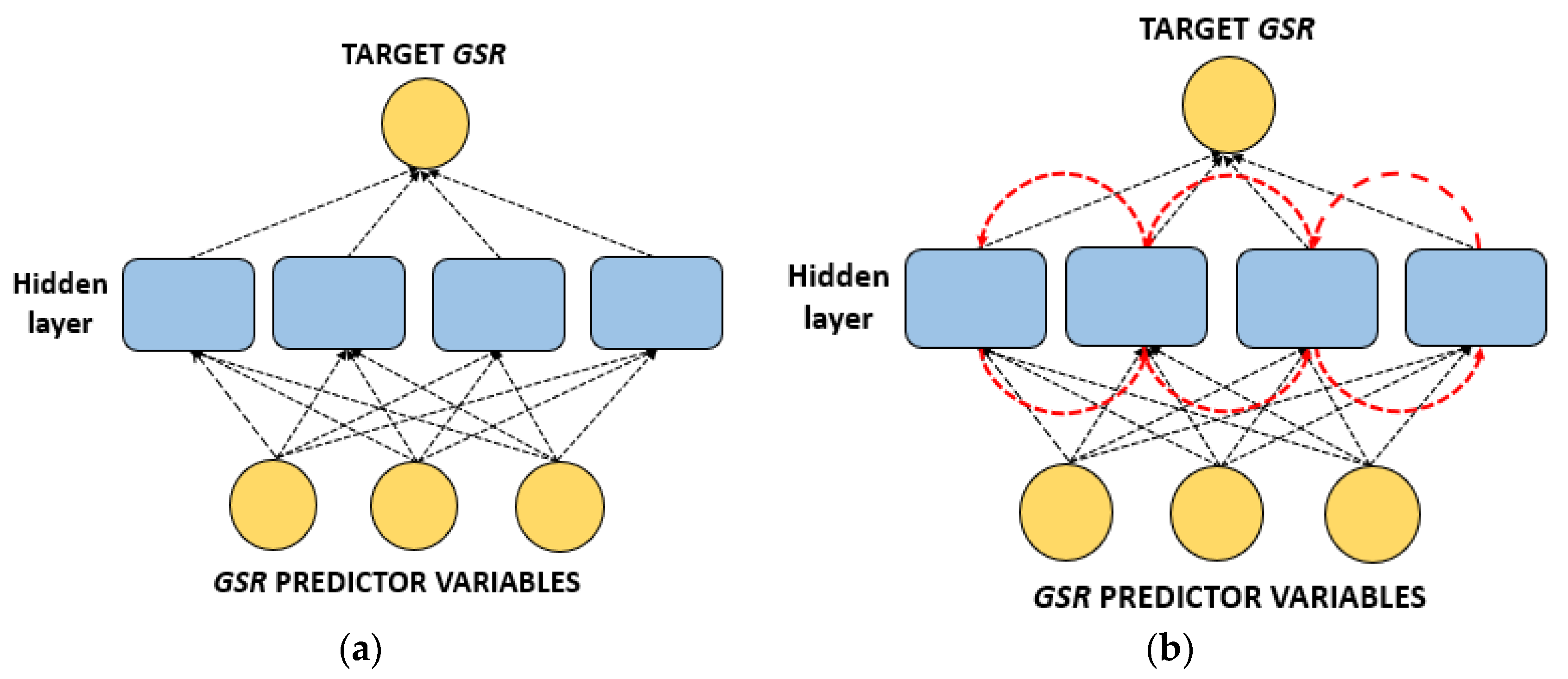
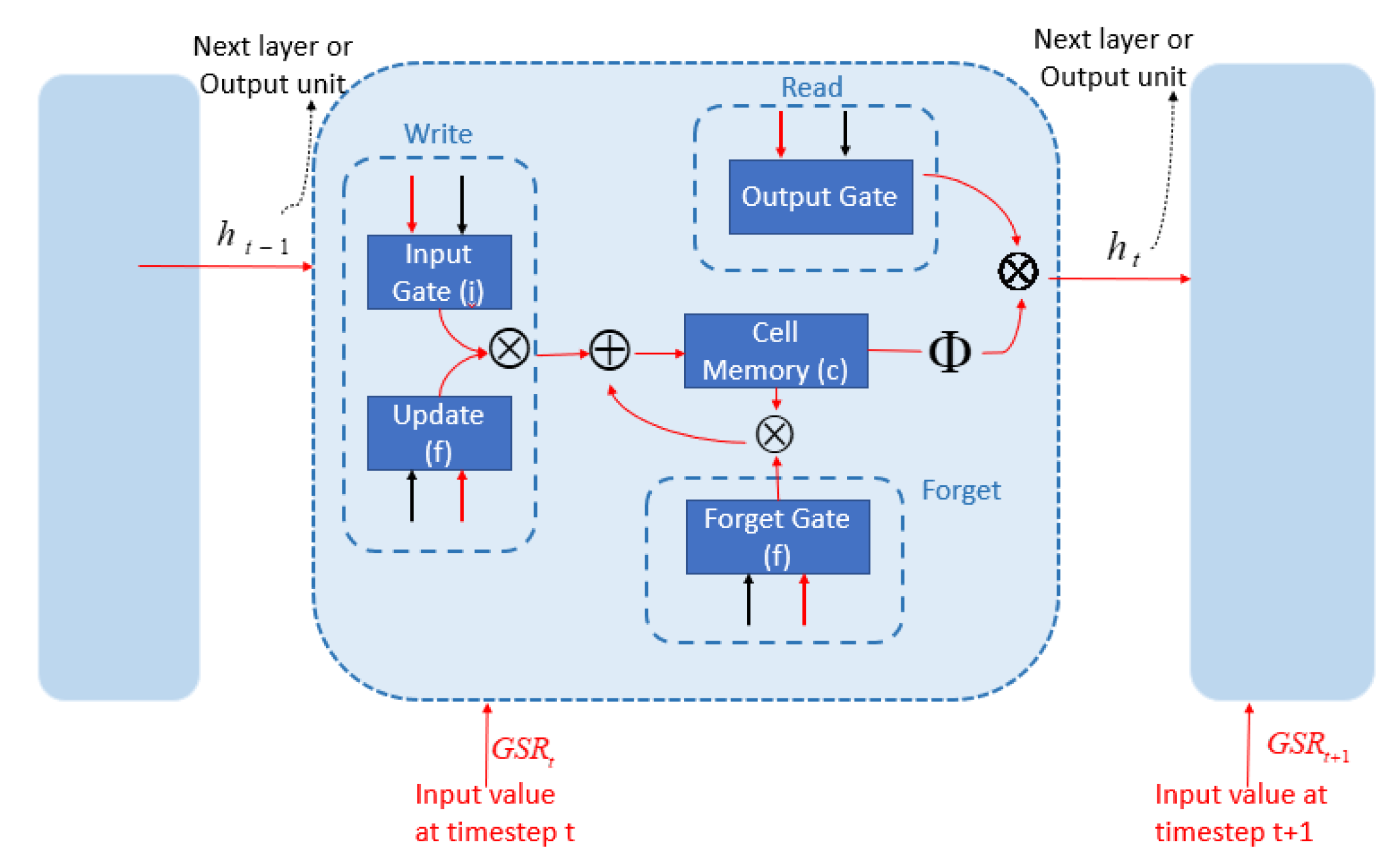
3.1. Objective Predictive Model: Long Short-Term Memory (LSTM) Network

The LSTM algorithm, used recently in solar radiation modelling is a branch of the deep recurrent neural network (RNN) (Figure 1a), which is an advanced method of machine learning, feed-forward neuron networks (FFNNs) (Figure 1b) [88]. Both models apply the idea of the human brain neuron network in which each neuron (blue colour) is an information processing unit. The improvement of RNN over FFNN is feedback loops (in red colour), which are units with memory. These units can remember, re-incorporate and update information from patterns learnt from previous steps, thus, RNN can learn progressively, rather than randomly, as is the case with FFNN. The previous state of the neuron, that is, the parameters of the previous time step, can be re-incorporated and taken into account when updating the memory. However, this property of RNN causes the vanishing gradient problem that prevents RNNs learning from deep sequences of broad contexts [89].

The long short-term memory (LSTM) algorithm was introduced by Hochreiter and Schmidhuber [90] in 1997 to address the vanishing gradient issue. Figure 2 illustrates the internal structure of LSTM with the innovative memory blocks called cells from which LSTM outperforms RNNs. From Figure 2, the transmission stage is between the previous hidden layer, the cell state and the next hidden layer. The cell state is the main chain of data flow, which allows the data to flow forward essentially unchanged. However, in this cell, there are specific gates, which allow some linear transformations to occur. The main utility of the LTSM model applied in real-time modelling contexts is its capability to learn long-term dependencies among the consecutive events on a relative timestamp through incorporating self-connected “gates” in the hidden units. In the context of GSR, especially at multiple forecasting horizons in this study, this model is likely to capture more accurately the real-time dependence of the historical, the current and the future GSR values, to finally create a more representative modelling framework. The gates enable LSTM units to read, write and remove information in the memory. Thus, they allow LSTM to remember the relevant data patterns while removing the irrelevant data, hence, sustaining a constant and relatively low error level, unlike the ARIMA (and other time-series) statistical model that uses its error to propagate into the future timescale, and potentially induces the inherent inaccuracies in the testing phase.

In terms of solar energy forecasting and applications in real time, the LSTM model is expected to exploit the temporal and spatial dependence of antecedent GSR data, while utilizing the contextual information. Consequently, in recent years, the LSTM has been implemented in many fields, including solar energy prediction [55,58], although the present study is the first of its kind to develop and apply this model for Vietnam, and, in particular, at multiple forecasting horizons.

3.1.1. Computational Aspects of LSTM Network Model

To gain an in-depth understanding of LSTM, Figure 2 illustrates a single localized LSTM cell in the first layer of a network at the timestep t. Symbols $\otimes$ and $\oplus$ represent point-wise scalar multiplication and summation, respectively. The colour arrows $\downarrow \downarrow$ show direction of input to the systems. $\Phi$ is an activation function which sets the ReLU (rectified linear units) in this experiment. These units are known as the Input Gate, Update Gate, Output Gate, and Forget Gate, and they represent the output value at the separate gates [92]. The gates normally receive an input of the same LSTM unit’s output, but obtained at a previous time step ($h_{t-1}$). These gates also receive the input data related to the current time step ($x_t$) in order to emulate the future value of GSR at any given timestep. With the same structure as RNN, a novel Forget Gate function enables inappropriate information to be removed and forgotten, which resolves the gradient vanishing issues of the RNN algorithm when applied to a large dataset context.

Firstly, based on the last hidden state ($h_{t-1}$) and the new input $x_t$, LSTM possibly selects the information, which is to be processed from the cell state represented by the Forget Gate ($f$):

$$f_t=\sigma \left(w_f\times \left[h_{t-1},x_t\right]+b_f\right)$$

(1)

Secondly, the next step is to determine the information that is stored in the cell state. There is a new candidate $\widetilde{c_t}$ which is generated by $x_t$ and $h_{t-1}$ through a $\tanh$ layer. This new candidate is then scaled by the Input Gate i:

$$\widetilde{c_t}=\tanh (w_c\times \left[h_{t-1},x_t\right]+b_c)$$

(2)

$$i_t=\sigma \left(w_i\times \left[h_{t-1},x_t\right]+b_i\right)$$

(3)

Then, by combining the previous cell state $C$, both $C_{t-1}$ and $c_t$, in which the former is determined in the Forget Gate ($f$) and the latter is identified by the Input Gate ($i$) as Equation (4):

$$c_t=f_t\times c_{t-1}+i_t\times \widetilde{c_t}$$

(4)

The above three kinds of gates are not static. The recent state information $h_{t-1}$ and the current input $x_t$ are jointly determined by non-linear activation after linear combination.

Finally, in the output process, there are two steps. The Output Gate is known as a new gate which is responsible for deciding appropriate parts from the cell state to be outputted. The cell state $c_t$ is activated by tanh function, which is then filtered through multiplying by $o_t$. The multiplication result is the desired output $h_t$:

$$o_t=\sigma (w_o\times \left[h_{t-1},x_t\right]+b_o)$$

(5)

$$h_t=o_t\times \tanh (c_t)$$

(6)

where $w_f,w_i,w_c,w_o$ are weight matrices, $b_f,b_i,b_c,b_o$ are bias vectors. σ () is the sigmoid activation function.

3.1.2. Benchmark Model: Autoregressive Integrated Moving Average (ARIMA)

This study also adopts the autoregressive integrated moving average (ARIMA) model to further validate the efficacy of the LSTM Network model. The ARIMA model was popularized by the work of Box and Jenkins [93]. ARIMA analyses a set of (univariate) predictor data partitioned into a subset of input/target to validate the LSTM and other models. Using its own time-lagged information and the respective model errors, ARIMA can identify the intermittent and chaotic patterns of original GSR time-series data, which is an alternative effective skill when other methods (e.g., LSTM or others) are not available.

An ARIMA model includes three parameters (p, d, q), with p as the number of autoregressive terms, d as non-seasonal differences and q as the number of lagged errors. The ARIMA process generally involves model identification, estimation and forecasting, defined as follows:

$${\psi }_p(B){(1-B)}^d{Y}_t=\delta +{\theta }_q{(B)}_{{\epsilon }_t}$$

(7)

in which ${\psi }_p$—the autoregressive parameter of order p; B—the backshift operator; $Y_t$—the original predictor dataset; $\delta$—constant value; ${\theta }_q$—the moving average parameter q; and d is the differencing order used for the regular or non-seasonal part of the series.

In the identification of an ARIMA model, the differencing parameter (d) is analysed by autocorrelation and partial autocorrelation to decide whether the differencing effect should be performed in a non-stationary dataset. Furthermore, p and q terms are identified for the model by analysing maximum likelihood estimation, which determines parameters maximising the probability of data by least squares. There are various terms (e.g., log likelihood, Akaike’s information criterion (AIC), Bayesian information criterion (BIC), r, RMSE) to determine the maximum combination of (p, d, q). Expressions of AIC and BIC are as follows:

$$AIC=-2\log (L)+2(p+q+k+1)$$

(8)

$$BIC=-2\log (L)+(p+q+k)\ast (p+q+k+1)\log (n)$$

(9)

where L is the log likelihood of data, k = 1 if c = 0 and k = 0 if c = 0; n is the sample size. The last term in brackets is the number of parameters (including the variance of the residual).

A detailed description of the ARIMA model can be found elsewhere and further applications of this method can be found in other’s works [31,94,95]. Generally, the ARIMA model assumes a scenario where there is no change in consecutive periodical measurements or the readings used to construct a model. Given that previous studies have employed an ARIMA model for GSR forecasting, this technique is also employed in this study in the interest of its ability in capturing historical patterns from the present time-series data.

3.1.3. Benchmark Model: Support Vector Regression (SVR)

Support vector regression (SVR) is a regression version of the SVM model that is usually applied in solar energy forecasting [96,97]. SVR transforms the original feature space into a high-dimensional one using a hyperplane which employs kernel functions (e.g., Gaussian, linear) to effectively separate data [98]. Herein, SVR is implemented using Python environment version 3.6 using the Sklearn library which is optimized using a grid search procedure.

3.1.4. Benchmark Model: Deep Neural Network (DNN)

The deep neural network is a machine learning method that has been advanced based on artificial neural networks (ANN), and is capable of trained complex input and learning procedures [45]. Similar applications of DNN in solar energy forecasting can be found in [17,99]. Herein, the deep learning library of Python retrieving solar radiation is applied. Like other neural network methods, the employed model comprised one input/output layer and multiple hidden layers. Various structures of the deep neural network were analysed to determine an optimal training model.

3.1.5. Benchmark Model: Multilayer Perceptron Network (MLP)

The multilayer perceptron network (MLP) is the most common type of feed-forward network [100]. MLP has three layers: an input layer, an output layer and a hidden layer. In this paper, MLP is implemented by the Python environment version 3.6 using the deep learning library. As for LSTM and DNN, various structures of MLP were analysed to determine an optimal training model.

4. Materials and Method

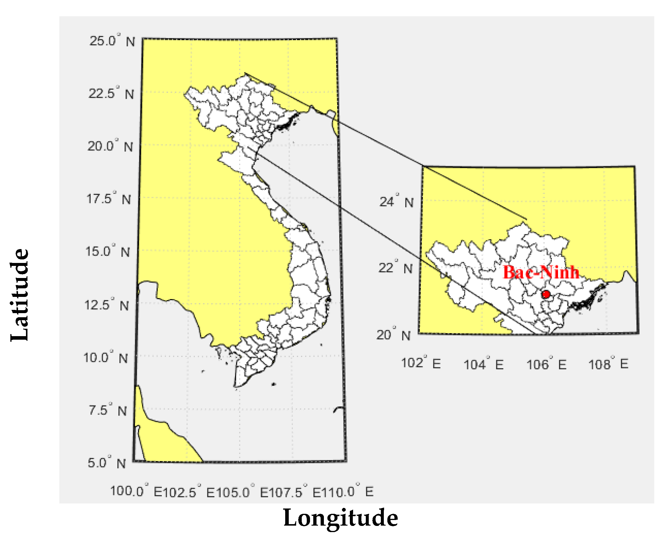
4.1. Study Region

The data utilized to build and evaluate the proposed LSTM network model comprised the minute interval time-series of global solar radiation (GSR), acquired from the reliable source of World Bank repositories from September 2017 to June 2019. The Vietnam government aims to develop large solar plants near its capital city that can reduce load emissions and avoid a downwind situation. A chosen location, the Bac-Ninh region (Figure 3), is a small city with about 100,000 people. The city is located in the North of Vietnam, not far from the capital, at latitude 21.2013° N and longitude 106.0629° E, and elevation of 60 m above sea level. The Bac-Ninh site has a subtropical dry winter climate characterized by hot and humid summers with frequent tropical downpours of short duration, and warm and frequently dry winters [101]. This province is undergoing revitalization in terms of more sustainable future solar energy systems, which are partly funded by the World Bank. The province also meets the criteria set for the selection of the present study location for the future installation of solar measurement stations, i.e., it is solar-rich with terrain either flat or characterised by low obstructions, homogeneous landscape and land-usage (clearly represented by satellite pixels for validation), without large water bodies, mountains, dirt roads, industrial pollution, open-pit mining operations, or a danger of flooding [102,103]. Thus, the development of a solar forecasting model at multiple forecast horizons, especially in Bac-Ninh, is a justified research endeavour to support the United Nation’s Sustainable Development Goal #7 related to the access to affordable renewable energies for all populations.

4.2. Data Preparation

This section details the activities of related to data preparation, including the construction of multiple time-scale datasets using 1 min original measurements, the handling of missing data, and the input of those data structures into the LSTM network. Notably, GSR measurements were performed simultaneously, 24 h a day, at equidistant time intervals of 1 min. Only the data from 06:00 to 18:00 were used for designing the predictive model as these times represent a period of meaningful daylight hours.

With the aim to construct a framework for a near-real-time prediction model, the raw 1 min time-series data were firstly used to generate the data at 5-, 10- 15- and 30 min-ahead time-series data, which were then used as the target variable. Details of those data are presented in

Table 2. Descriptive statistics of the global solar radiation (GSR) dataset aggregated at various timescales for the Bac-Ninh region in Vietnam used to develop the prescribed LSTM model tested at multiple forecast horizons.

Forecasting Horizon	Data Period	Minimum Wm−2	Maximum Wm−2	Mean Wm−2	Standard Deviation Wm−2
1 min (1 M)	1 June 2019 to 30 June 2019	0	1376	207	283
5 min (5 M)	1 March 2019 to 30 June 2019	0	6047	730	1157
10 min (10 M)	27 September 2017 to 30 June 2019	0	11,889	1416	2297re
15 min (15 M)	27 September 2017 to 30 June 2019	0	16,574	2124	3430
30 min (30 M)	27 September 2017 to 30 June 2019	0	32,042	4249	6804

.

With respect to the missing data, it is noted that missing values represent only 0.15% of the time-series data, and were due to equipment faults or site closures in the measured period. We imputed those missing values by the mean value of the whole period [95,104]. Clearly, more powerful techniques (e.g., step-wise linear regression fit, Kalman filters) could be considered and might facilitate better imputation but given the relatively low percentage of missing data, these may not be required in this study. Moreover, these data are employed for the comparison of LSTM with the other models. Consequently, the imputation method should not influence the relative performance of the alternative forecasting methods.

To prepare the suitable number of inputs for each time-scale horizon (based on historical behaviour of short-term solar radiation measurements), the autocorrelation coefficient and the partial correlation coefficient (PACF) were employed. The detailed procedures can be found in [94]. Explicitly, the PACF function computes a time-series regression against its n-timescale lagged values by removing the dependency on intermediate elements and identifying those patterns potentially prevalent in the future GSR data that are correlated to the antecedent GSR data. This procedure aims to develop forecast models that consider the role of memory (i.e., antecedent GSR) adopted in forecasting the current GSR value, and possibly, considers several other atmospheric factors that could potentially influence ground level GSR. Consequently, the input vector $GS{R}_{t-1},GS{R}_{t-2},\dots ,GS{R}_{t-n}$, called the n-lagged set of inputs deduced from the PACF method, was then used as the LSTM model’s input to predict the GSR as the target. Figure 4 shows the PACF plot of GSR time series with lagged inputs as predictor variables for the LSTM model applied at 1 M, 5 M, 10 M, 15 M, and 30 M forecast horizons.

The primary scope of this study is to design, for the first time in the present study region, an LSTM model that has the capability to forecast near real-time GSR using minute interval data, applied for multi-step forecasting horizons. To expand the practical scope of the modelling techniques, the developed model was applied at 1 min (1 M), 5 min (5 M), 10 min (10 M), 15 min (15 M) and ½ hourly (30 M) forecasting horizons, to enable LSTM to generate a more granular interval GSR, as required in real-life decisions, for example, through constant monitoring of solar energy resources. Hence, the primary task is to construct a matrix of a training and testing dataset that can reliably be applied to the proposed LSTM model.

The normalization of modelled data was accomplished by statistical rules to overcome the numerical difficulties caused by the data features, patterns and fluctuations using the conventional methods of feature scaling [105]. Normalization is applied to the n-lagged inputs [9] to be in the range of [0–1] by the following formula:

$$GS{R}_N=\frac{GS{R}_{ACTUAL}-GS{R}_{MIN}}{GS{R}_{MAX}-GS{R}_{MIN}}$$

(10)

$$GS{R}_{ACTUAL}=GS{R}_N(GS{R}_{MAX}-GS{R}_{MIN})+GS{R}_{MIN}$$

(11)

After normalization, a major task was to determine the training data, to construct the predictive model, and the testing data, and thus achieve the highest performance. The partitioning of data followed the notion that researchers use different divisions between testing and training sets, which generally vary with the problem. There is no ‘rule of thumb’ for data divisions. In [58], the authors employed about 75% of inputs for training and the remainder for the testing set, while in [44] the partition proportion for training and testing sets was approximately 80:20. Subsequently, the normalized data are then divided into the training (80%) and testing (20%) sets (

Table 3. (a) Model designations and various input combinations based on the partial autocorrelation function used to identify antecedent lagged GSR for the objective LSTM and the comparative counterparts adopted at multi-step forecasting horizons. (b) Training phase results of LSTM with different partition proportions.

(a)
Forecast Horizon	Significant Lagged GSR	Number of Data Point	Training	Validation	Testing
			80%	Percentage of Training Data	20%
1 M	18	43,197	34,558	10%	8637
5 M	6	35,133	49,518		12,376
10 M	3	92,874	24,757		6187
15 M	19	61,897	34,558		8637
30 M	10	30,946	28,106		7025
(b)
Model	Training-Testing Proportion			r	RMSE (Wm−2)	MAE (Wm−2)
LSTM	80–20			0.9957	32.086	13.670
-	70–30			0.9901	43.7088	15.715
-	60–40			0.9799	60.9179	23.402

a). Noticeably, the number of data points is significantly higher than any of the previous relevant papers [15,64].

4.3. LSTM Model Implementation

Prior to developing the proposed LSTM-based solar radiation forecasting model, the historical GSR data were pre-processed at multiple forecasting time horizons. The proposed model-based LSTM was developed under the Python environment on an Intel Core i5 and 16 GB RAM computer.

The development and validation of the proposed method, as shown in Figure 5, is presented in the following steps:

Step 1: Construct the data matrix which is used as the input in the first layer. The statistically significant lags were calculated from the original GSR time series data using the partial autocorrelation function (PACF). In addition, to demonstrate data efficiency in this model, we also used different partition proportion in dividing training and testing sets (Table 3b). As a result, the scale of 80:20 represents the highest performance of the LSTM, therefore, this scale is appropriate in this study.

Step 2: After incorporating the significant lagged inputs as the input predictor, the LSTM was implemented using the Keras deep learning package in Python [106]. The input layer of the trained LSTM network had four timesteps; hidden neurons were set to 80; and the output layer with a linear activation function had one neuron. In addition to these fixed values, we ran the LSTM model with different combinations of hyperparameters (epoch-drop rate-batch size) which were selected through a grid search. Table 3a summarizes the general architecture of different types of LSTM by various combinations of hyperparameters. However, only those experiments for 1 M are shown.

Step 3: To select the optimal model for each case, the LSTM algorithm begins with the change of each hyperparameter. Then, based on the recorded evaluation metrics (r-value, RMSE) in the training phase, we selected the optimal LSTM model with the highest r-value and the lowest RMSE.

Table 4. (a) The architecture of the objective LSTM model with various model design parameters. Note that ReLU stands for rectified linear unit. (b) Experimental results of LSTM model in 1 M forecast horizon in the training phase. (c) The optimal architecture used in designing optimized LSTM vs. the comparative models (i.e., autoregressive integrated moving average (ARIMA), deep neural network (DNN), multilayer perceptron (MLP), support vector regression (SVR)) in the training phase.

(a)
Model	Model Hyperparameters	Search Space for Optimal Hyperparameters
LSTM	Hidden neurons	(100, 200, 300, 400, 500)
-	Epochs	(1000, 1200, 1500, 2000)
-	Optimizer	(Adam)
-	Drop rate	(0.1, 0.2)
-	Activation function	(ReLu)
-	Layer 1 (L1) and Layer 2 (L2), Layer 3 (L3)	(50, 40, 40)
-	Batch size	(400, 600, 700, 750, 800)
(b)
Sequence	Initial Set-Up Epoch	Actual Used Epoch	Drop Rate	Batch Size	r	RMSE (Wm−2)
1	2000	54	0.1	500	0.9874	33.201
2	2000	55	0.1	750	0.9875	33.178
3	2000	53	0.1	800	0.9884	33.098
4	2000	62	0.1	1000	0.9876	33.096
5	2000	64	0.2	800	0.9956	32.086
(c)
Time-Horizon	GSR Model	Design Parameter			r	RMSE (Wm−2)
1 M	LSTM	Number of epochs-Drop rate-Batch size		64-0.1-800	0.9956	33.2012
	DNN	Number of epochs-Drop rate-Batch size		162-0.1-500	0.990	44.0424
	MLP	-		-	0.9821	61.7642
	ARIMA	p-d-q		0-1-0	0.9808	57.6876
	SVR	Cost Function (C), Epsilon (ε)		1.0-1.0	0.9846	59.2223
5 M	LSTM	Number of epochs-Drop rate-Batch size		59-0.2-800	0.9714	265.5456
	DNN	Number of epochs-Drop rate-Batch size		199-0.1-500	0.9650	1338.4922
	MLP	-		-	0.9721	361.7641
	ARIMA	p-d-q		0-1-0	0.9724	287.7479
	SVR	Cost Function (C), Epsilon (ε)		1.0-1.0	0.9218	389.6317
10 M	LSTM	Number of epochs-Drop rate-Batch size		59-0.2-800	0.9914	26.4411
	DNN	Number of epochs-Drop rate-Batch size		194-0.1-500	0.9871	26.6411
	MLP	-		-	0.9599	26.3175
	ARIMA	p-d-q		0-1-0	0.9205	22.622
	SVR	Cost Function (C), Epsilon (ε)		1.0-1.0	0.9514	51.6976
15 M	LSTM	Number of epochs-Drop rate-Batch size		70-0.2-500	0.9653	76.9883
	DNN	Number of epochs-Drop rate-Batch size		162-0.1-500	0.9657	88.9887
	MLP	-		-	0.9547	220.7234
	ARIMA	p-d-q		0-1-0	0.9618	1033.4372
	SVR	Cost Function (C), Epsilon (ε)			0.8983	117.7362
30 M	LSTM	Number of epochs-Drop rate-Batch size		62-0.2-500	0.9572	710.7477
	DNN	Number of epochs-Drop rate-Batch size		28-0.1-700	0.9067	709.0347
	MLP	-		-	0.9192	900.1132
	ARIMA	p-d-q		0-1-0	0.8859	952.8502
	SVR	Cost Function (C), Epsilon (ε)		1.0-1.0	0.8314	1270.7158

b presents the experimental results in the training phase with the optimal models highlighted in red. However, only those experiments for 1 M are shown. After conducting all experiments, the summarized results of the optimal model for all forecasting time horizons (1 M, 5 M, 10 M, 15 M and 30 M) are shown in Table 4c.

For the case of an LSTM network model, the computational cost is considered to be an important aspect in terms of learning process [107], which is directly influenced by the dataset size in the training phase [107] and the respective hyperparameters [108]. To reduce the high computational cost in the learning process of the objective (i.e., LSTM) model, the hyperparameters for the model are chosen through a grid search process for the optimal parameters; however, this can be relatively time-consuming. For instance, for each LSTM model, the search took about 11–12 h; however, when the optimal hyperparameters are determined prior to running the primary LSTM model, the computational time of the model was reduced to a much lower value (<15 min).

Generally, a hyperparameter is a parameter whose value is set before the learning process commences. There are two types of hyperparameters, namely, model hyperparameters (e.g., the size of the neural network and the number of input layers in FFNNs) and algorithm model hyperparameters (e.g., dropout and batch size). Model hyperparameters cannot be inferred during the training process since this must be referred to the model selection task. The latter, algorithm hyperparameters, in principle, can increase the speed and quality of the learning process. Therefore, determining the most appropriate hyperparameters is essential for the success of a deep learning model such as the LSTM model adopted in this study. Depending on the model types, strategies for choosing hyperparameters may vary. While some of the hyperparameters are model-specific, some common hyperparameters that can be used in any deep learning model, and that were also adopted in this study, are:

• Epoch defines the number of times that the learning algorithm will work through the entire training dataset. The number of epochs is usually hundreds or thousands, allowing the learning algorithm to run until the error from the learning model is minimized. In this study, the number of epochs is set to a maximum of 2000 (Table 4).
• Batch size defines the number of data points that are propagated through the network. The batch size can be seen as a for-loop iterating over one or more data points. At the end of each batch, the predicted values are compared to the actual values and the errors are calculated. From these errors, the update algorithm is used to improve the model. Depending on data length, to determine whether a greater batch size can provide the better performance, the batch size is set as in Table 3.
• Dropout is a regularization layer that blocks a random set of cell units in one iteration of LSTM training. Since over-fitting is prone during training, the dropout layer creates blocked units which can remove connections in the network. Therefore, it possibly decreases the number of free data points to be predicted and the complexity of the network. The dropout rate is often set between 0 and 1. In this study, this parameter was tested between two values, 0.1 and 0.2, to determine whether a greater value of dropout rate improves LSTM performance (Table 4a).
• Least absolute deviations and least square error (L1 and L2 regulation): In addition to dropout, the L1 and L2 regularization parameter is also used such that the L1 and L2 penalization parameter decreases the sum of absolute differences and the sum of square of differences between observed and forecasted values. In principle, adding a regularization term to the loss will facilitate a better network mapping (by penalizing large values of parameters which minimize the amount of nonlinearity of GSR values).
• Activation function: With the exception of the output layer, all the layers within a network typically use the same activation function known as the rectified linear unit (ReLU).

4.4. Benchmark Models Implementations

To comprehensively evaluate the optimal LSTM forecasting model, five other popular forecasting models based on the ARIMA, DNN, MLP, and SVR algorithms were developed under the Python environment, version 3.6, on an Intel Core i5 computer. For the purpose of brevity and conciseness, only the results at the 1 min (1 M) forecasting horizon are shown here, but the results obtained at the other forecasting horizons resulted in relatively similar deductions. Finally, following the previous steps, the optimal models based on the LSTM versus the counterpart models are shown in Table 4c for a diverse range of forecasting horizons.

5. Model Performance Criteria

Several methods have been previously adopted to evaluate model performance [109]. In the present work, a popular set of statistical metrics (e.g., bias, mean square error, linear correlation coefficient) are employed to assess the model performance since each individual metric has its own strength and weakness [110]. For instance, due to the standardization of observed and forecasted means and variance, the robustness of Pearson’s correlation coefficient (r), which exceeds 1 as the perfect model, may have limited meaning [70,95]. Moreover, while root mean square error (RMSE) is relevant for high values, mean absolute error (MAE) assesses all deviations of observed data both in the same manner and regardless of sign [111]. RMSE and MAE are recommended to address each other’s weaknesses and to obtain accuracy in an absolute unit [111]. The performance of a model can be decreased because of partial peaks and higher magnitudes, which may cause large errors and be insensitive to small magnitudes. To solve this problem, efficiency measurement indexes, such as Willmott ($WI$) and Nash-Sutcliffe ($E_{NS}$) [112] are introduced with the advantage of overcoming insensitivity and over-dominance of significant errors over small errors [113,114]. Nevertheless, $E_{NS}$ is relatively high even in the poorly-fitted models and vice versa, hence, it can confuse performance evaluation [115]. Therefore, $WI$ is implemented to be incorporated with $E_{NS}$ [112].

However, a certain degree of insufficiency still occurs with $WI$ that can be improved by the Legate and McCabe index (LM) [116]. Since different forecasting horizons can lead to differences in data distribution, the relative root mean square error (RRMSE) [117] and mean absolute percentage error (MAPE) [118] are computed since they are also the benchmark of evaluating a “good” model. A model’s precision level is excellent if RRMSE < 10%, good if 10% < RRMSE < 20%, fair if 20% < RRMSE < 30%, and poor if RRMSE > 30% [117]. Therefore, to properly assess model performance, in this paper, several statistical score metrics are exploited, such as the Pearson’s correlation coefficient (r) [119], root mean square error [120] (RMSE; ${\mathrm{Wm}}^{-2}$), mean absolute error [121] (MAE; ${\mathrm{Wm}}^{-2}$), including the relative error values: RMSE (RRMSE; %), MAE, MAPE, $WI$, and $E_{NS}$, which are adopted as the well-known metrics employed elsewhere (e.g., [79]).

$$r={\left(\frac{{\displaystyle \sum _{i=1}^n(GS{R}^{OBS}-⟨GS{R}^{OBS}⟩)(GS{R}^{FOR}-⟨GS{R}^{FOR}⟩)}}{\sqrt{{\displaystyle \sum _{i-1}^N{(GS{R}^{OBS}-GS{R}^{OBS})}^2}}\sqrt{{\displaystyle \sum _{i-1}^N{(GS{R}^{FOR}-GS{R}^{FOR})}^2}}}\right)}^2$$

(12)

$$MAE=\left({\displaystyle \sum _N^{t=1}\left|GS{R}^{OBS}-GS{R}^{FOR}\right|}\right)/N$$

(13)

$$RMSE=\sqrt{\frac{1}{N}{\displaystyle \sum _{i=1}^N{(GS{R}^{OBS}-GS{R}^{FOR})}^2}}$$

(14)

$$E_{NS}=1-\frac{{\displaystyle \sum _{i-1}^N{\left[GS{R}^{OBS}-GS{R}^{FOR}\right]}^2}}{{\displaystyle \sum _{i-1}^N{\left[GS{R}^{OBS}-GS{R}^{FOR}\right]}^2}},-\infty \le E_{NS}\le 1$$

(15)

$$WI=1-\frac{{\displaystyle \sum _{i-1}^N{\left[GS{R}^{OBS}-GS{R}^{FOR}\right]}^2}}{{\displaystyle \sum _{i-1}^N{\left[\left|(GS{R}^{FOR}-(GS{R}^{OBS}))\right|+\left|(GS{R}^{OBS}-(GS{R}^{FOR}))\right|\right]}^2}},0\le WI\le 1$$

(16)

$$LM=1-\frac{{\displaystyle \sum _{i=1}^n\left|GS{R}^{OBS}-GS{R}^{FOR}\right|}}{{\displaystyle \sum _{i=1}^n\left|GS{R}^{OBS}-⟨GS{R}^{OBS}⟩\right|}},-\infty \le LM\le 1$$

(17)

$$MAPE=({\displaystyle \sum _N^{t=1}\left|(GS{R}^{OBS}-GS{R}^{FOR})/GS{R}^{OBS}\right|})/N$$

(18)

$$RRMSE=\frac{\sqrt{\frac{1}{N}{\displaystyle \sum _{i=1}^N{(GS{R}_i^{FOR}-GS{R}_i^{OBS})}^2}}}{\frac{1}{N}{\displaystyle \sum _{i=1}^{N}GS{R}_i^{OBS}}}\times 100$$

(19)

6. Statistical Significance Testing

Based on performance metrics it is difficult to conclude whether the results are due to chance or decisive. We possibly reject a factually good parallel model since the performance metrics might be generated stochastically. Consequently, from a statistical perspective, a significant difference of forecasting performance cannot be solely judged by traditional performance metrics. Therefore, this paper employed a modern statistic evaluation method, the Diebold–Mariano (DM) test [122], which can offer a quantitative method to evaluate the forecast accuracy of forecasting model. The DM test is applicable to nonquadratic loss functions, multi-period forecasts and forecast errors that are non-Gaussian and nonzero-mean. Details of the DM test can be found in [122] and some applications of the DM test can be found in [123,124]

Finally, with the help of the DM test, the interference by sample stochastic difference can be revealed, such that the better forecasting model can be identified statistically. To determine whether one forecasting model is better than another, we might first test the equal accuracy hypothesis. A null hypothesis ($h_o$) means that the observed differences between the performances of two forecasting models are not significant. An alternative hypothesis (h₁) means that the observed differences between the performances of two forecasting models are significant. Since the DM statistics converge to a normal distribution, we can reject the null hypothesis at the 5% level of significance if |DM| > 1.96, otherwise, we cannot reject the null hypothesis ($h_o$). If the DM statistic value does not meet the acceptable criterion, then the null hypothesis cannot be accepted, i.e., the two forecasts are statistically not different. By comparing LSTM to each counterpart in turn, it can be concluded whether the LSTM model is superior than its counterparts.

7. Results and Discussion

In this section, the experimental results and the overall performance assessment at different forecasting horizons are presented. For each modelling experiment, five GSR forecasting models, including the proposed LSTM model and the counterpart models (i.e., ARIMA, DNN, MLP, and SVR) are employed. To demonstrate the merits of the LSTM model over the counterpart models in terms of their near-real-time solar forecasting capability, a plethora of model evaluation metrics for the testing phase, as described by Equations (9)–(16), is presented in

Table 5. The model performance in the testing period as measured in terms of correlation coefficient (r), root mean squared error (RMSE), mean absolute error (MAE).

Predictive Model	r					RMSE ${\mathbf{Wm}}^{-2}$					MAE ${\mathbf{Wm}}^{-2}$
	1 M	5 M	10 M	15 M	30 M	1 M	5 M	10 M	15 M	30 M	1 M	5 M	10 M	15 M	30 M
LSTM	0.9920	0.9999	0.9999	0.9578	0.9531	40.9125	1400	18.6627	79.7273	731.7482	21.6428	1059	12.3368	43.8383	409.7196
MLP	0.9780	0.9266	0.9062	0.9246	0.8554	65.7511	1852	88.9537	218.7543	1254.3440	34.2960	1326	53.8914	106.8205	778.1039
DNN	0.9910	0.9606	0.9998	0.9568	0.9094	44.4086	1570	61.8762	86.6580	940.4280	25.5140	1134	40.9027	49.0178	576.9220
ARIMA	0.9902	0.9607	0.9989	0.9584	0.9094	52.9785	1589	37.8037	161.1655	937.1356	31.9632	1149	24.9898	100.5221	571.3325
SVR	0.9856	0.9266	0.9358	0.9247	0.8555	56.1271	1619	74.8298	99.9360	1244.6963	31.5000	1136	42.1483	70.2232	773.6047

,

Table 6. The model performance in the testing period as measured in terms of Willmott’s index (WI), Nash–Sutcliffe Efficiency ($E_{NS}$) and relative root mean square error (RRMSE).

Predictive Model	WI					${\mathit{E}}_{\mathit{N}\mathit{S}}$					RRMSE (%)
	1 M	5 M	10 M	15 M	30 M	1 M	5 M	10 M	15 M	30 M	1 M	5 M	10 M	15 M	30 M
LSTM	0.9984	0.9409	0.9989	0.9770	0.9811	0.9831	0.6420	0.9920	0.8712	0.8931	9.9278	51.7123	10.1362	42.1591	41.0858
MLP	0.9959	0.8816	0.9721	0.9167	0.9347	0.9563	0.3737	0.8188	0.0306	0.6859	15.9581	68.3986	48.3132	115.6755	70.4282
DNN	0.9981	0.9227	0.9844	0.9717	0.9718	0.9800	0.5500	0.9123	0.8479	0.8235	10.7782	57.9785	33.6067	45.8240	52.8026
ARIMA	0.9972	0.9202	0.9947	0.9500	0.9700	0.9716	0.5386	0.9673	0.4738	0.8247	12.8582	58.7073	20.5322	85.2231	52.6178
SVR	0.9969	0.9179	0.9801	0.9635	0.9364	0.9681	0.5212	0.8718	0.7977	0.6907	13.6223	59.8060	40.6421	52.8454	69.8865

and

Table 7. The model performance in the testing period as measured in terms of the Legates and McCabe index (LM) and mean absolute percentage error (MAPE).

Predictive Model	LM					MAPE (%)
	1 M	5 M	10 M	15 M	30 M	1 M	5 M	10 M	15 M	30 M
LSTM	0.9204	0.4658	0.9275	0.7575	0.7741	16	48	100	86	116
MLP	0.8739	0.3311	0.6832	0.4090	0.5710	47	54	127	143	49
DNN	0.9062	0.4279	0.7596	0.7288	0.6819	49	58	60	62	67
ARIMA	0.8825	0.4203	0.8531	0.4438	0.6850	233	267	151	127	85
SVR	0.8842	0.4272	0.7522	0.6115	0.5734	56	91	143	120	262

.

For all of the modelling experiments capturing the highest Pearson’s correlation coefficient (r), the lowest root mean square error (RMSE), and the lowest mean absolute error (MAE), the proposed LSTM model achieves better results than the counterpart models executed for multiple time horizons. In particular, the LSTM model-simulated 1 M forecast horizon outperforms all of the other developed models with the statistics r = 0.9920, RMSE = 40.9125 ${\mathrm{Wm}}^{-2}$, and MAE = 21.6428 ${\mathrm{Wm}}^{-2}$ vs. r = [0.9920, 0.9780], RMSE = [40.9125, 65.7511], and MAE = [21.6428, 34.2960] where [] represents the upper and lower bounds of the metrics for the various models.

Figure 6 illustrates scatterplots for the observed and the forecasted GSR values of the developed models for the 1 M horizon. In each panel, the coefficient of determination ($R^2$) and a linear fit equation ($GS{R}^{OBS}=mGS{R}^{FOR}+c$) are shown to demonstrate the coherence between forecasted and observed GSR [104]. Here the constants—‘m’ (gradient) and ‘c’ (intercept on the y-axis)—and $R^2$ are utilized to outline the models’ overall accuracy. Note that $R^2$ and m values close to 1.00 and c value close to 0 should be attained for a perfect forecasting model. Evidently, the LSTM model achieves a better degree of agreement than the corresponding counterpart models. Moreover, to demonstrate the LSTM model’s outstanding performance in predicting the GSR data in the testing phase, Figure 6 also shows a time-series plot for all of the study cases, for which the forecasted values of LSTM (in red) appear to be closer to the observed GSR values (in blue) compared to those of the counterpart models.

To further explore the precision of the proposed LSTM model, Table 6 presents the metrics evaluating the forecasting errors (i.e., RRMSE, LM and MAPE). As can be seen, the proposed LSTM model is seen to outperform the counterpart models in all of the study cases in terms of the lowest RRMSE and MAPE and the highest value of the LM index. Evidently, the LM values produced by LSTM for all of the multiple forecasting horizons outperform those of both of the counterpart models. For instance, LM in the 1 M model is 0.9204, whereas those of counterpart models (i.e., MLP, DNN, ARIMA, and SVR) are 0.8739, 0.9062, 0.8825, and 0.8842, respectively. While it is argued that RRMSE is limited in the context of a dataset with the same variance, in our case, the RRMSE value clearly shows us which model would be better in terms of producing fewer and relatively low-magnitude errors [125]. Thus, LSTM certainly performs better than the counterpart models as it generated an RRMSE that is lower than that of the comparative models. Meanwhile, in terms of the MAPE value, the results of the proposed LSTM over multiple time horizons yield values of 16%, 48%, 100%, 86% and 116%, respectively, implying that the LSTM does not perform particularly well. However, the disadvantage of MAPE, which could perhaps explain this result, is that it generates a substantial percentage error for near-zero observed values as infinite MAPEs, and this effect can be quite pronounced if the observed GSR values are less than 1 [126]. This is a reasonable explanation for low performance in terms of MAPE since GSR time-series data, particularly at the very short-term time-scales used in this study, are expected to intermittently contain numerous near-zero values in the morning as observed elsewhere [125].

Figure 7 illustrates the boxplots for the case of the 1 M model that depict the different forecasting skills regarding the absolute prediction error (i.e., forecasted—observed GSR values). The lower and upper lines of the boxplot denote the first and third quartile values (25th and 75th percentiles), respectively, and the median value (50th percentile) is represented by the central line. Additionally, two horizontal lines are also drawn from the first and third quartiles to the smallest and largest non-outliers, respectively. To concur with earlier results, the boxplot provides further justification that the distributed errors for the proposed LSTM model also acquire a much smaller spread with a correspondingly smaller magnitude of the quartile statistics and median values compared to the MLP, DNN, ARIMA, and SVR models.

Lastly, to consolidate the findings presented so far that demonstrate the efficacy of LSTM model, a Taylor diagram that determines the angular location to the inverse cosine of the correlation coefficient is presented in Figure 8 to show the closest model in respect to the observed data in the testing period. The correlation coefficient (r), on the radial axis, and the standard deviation, on the polar axis, are used simultaneously to judge the closest fitting model. For all different timescales, the LSTM generates the highest value of r, with the forecasted results being closest to the observed data compared to the other comparative approaches.

In addition, the forecasting performance of the five models is compared by the DM test (Section 5). The forecasting comparison of every pair of models is summarized in

Table 8. Diebold–Mariano (DM) test adopted to compare the predictive accuracy of any two forecasting models. The objective model (i.e., LSTM) is compared against counterpart models (ARIMA, MLP, DNN and SVR) in the testing phase. The DM test is used to evaluate if the two forecasts are statistically different with a null hypothesis of no difference rejected if the test statistic falls outside DM = ±1.96 at a 5% level of significance. The statistically significant better performance of LSTM over the other models is indicated as ‘yes’.

Diebold–Mariano (DM) Test Statistics Forecast Horizon	LSTM vs. DNN	LSTM vs. ARIMA	LSTM vs. MLP	LSTM vs. SVR
1 Min (1 M)	-	-	-	-
DM statistic	−0.272	−24.381	−25.824	−16.933
p-value	0.785	0.000	0.000	0.000
Reject Null Hypothesis	No	Yes	Yes	Yes
5 Min (5 M)	-	-	-	-
DM statistic	46.585	46.394	−50.779	43.614
p-value	0.000	0.000	0.000	0.000
Reject Null Hypothesis	Yes	Yes	Yes	Yes
10 Min (10 M)	-	-	-	-
DM statistic	62.231	27.318	62.231	32.816
p-value	0.000	0.000	0.000	0.000
Reject Null Hypothesis	Yes	Yes	Yes	Yes
15 Min (15 M)	-	-	-	-
DM statistic	−51.638	−29.999	39.581	−0.268
p-value	0.000	0.000	0.000	0.789
Reject Null Hypothesis	Yes	Yes	Yes	No
Half Hourly (30 M)	-	-	-	-
DM statistic	−9.209	18.234	−19.558	17.000
p-value	0.000	0.000	0.000	0.000
Reject Null Hypothesis	Yes	Yes	Yes	Yes

. The null hypothesis means that the two forecasts have the same accuracy, otherwise, the two forecasts have different levels of accuracy in the alternative hypothesis. The statistically significant better performance of LSTM over the counterparts is indicated as ‘yes’. From Table 8, the conclusions of comparison of the LSTM model and the counterparts (i.e., DNN, MLP, ARIMA and SVR) can be drawn as follows. Firstly, since the absolute value of the DM statistic in most cases is greater than 1.96, the null hypothesis is rejected at the 5% level of significance; that is to say, the observed differences are significant and the forecasting accuracy of LSTM models is better than that of the counterparts. The exceptions are the comparison of LSTM vs. DNN at the 1 M forecast horizon and that of LSTM vs. SVR at the 15 M forecast horizon, with corresponding absolute DM statistics of 0.272 and 0.268, respectively, which are less than 1.96. This shows the performance of LSTM vs. DNN and LSTM vs. SVR are not significant and might be due to stochastic interference. These clearly prove that the LSTM models receive more significance than the others. In addition, the p-value at a 5% level of significance is less than 0.05, which means all models are statistically significant.

In summary, by an evaluation of forecasting based on performance metrics and the DM test, the LSTM model was demonstrated to outperform the comparative models. Thus, it is found to be a versatile solar forecasting tool, especially over short-term, multiple timescale horizons.

8. Further Discussion, Limitations and Future Scope

Despite the excellent performance of the developed LSTM model, as evaluated by several statistical metrics and visualized model analysis, the proposed model is further evaluated by comparing the results in this study with those of previous studies. In one such study, an LSTM model was developed for 1-hourly day-ahead solar irradiance forecasting on the island of Santiago, Cape Verde. The study employed weather variables (i.e., temperature, dew point, humidity, visibility, wind speed, weather type) for 30 months (March 2011 to August 2012). In concurrence with the present study (Table 5), it was concluded that the LSTM model was the best model as it generated the lowest RMSE in comparison to the persistence, ANN, and linear least squares regression methods (76.245 ${\mathrm{Wm}}^{-2}$, 209.2509 ${\mathrm{Wm}}^{-2}$, 230.9857 ${\mathrm{Wm}}^{-2}$, and 133.5313 ${\mathrm{Wm}}^{-2}$, respectively).

Another relevant comparative study employed LSTM to estimate hourly and daily GSR in Atlanta, New York, and Hawaii using hourly meteorological data and cloud type information from 2013 to 2017 as a training and testing population. The proposed LSTM demonstrated excellent forecasting performance for hourly forecasts on all-weather (i.e., mixed days and cloudy days). The mean absolute percentage error (MAPE) of LSTM in measured locations (i.e., Atlanta, New York, Hawaii) on cloudy days was 14.9%, 20.1% and 18.1% respectively. All r-values of LSTM were above 0.85, outperforming comparative models (i.e., ARIMA, SVR, ANN, CNN, and RNN) with one exceptional case where the r-value of RNN was higher than that of LSTM (0.91 and 0.90, respectively). Overall, however, LSTM showed its outstanding performance. The study of Ghimire et al. [44] designed a hybridized framework that integrated a convolutional neural network with LSTM for half-hourly GSR forecasting in Australia; their model was superior, with over 70% of predictive errors lying below ±10 ${\mathrm{Wm}}^{-2}$. The results from the last two studies are the only close available comparisons of solar forecasting studies employing LSTM. Regarding the evaluation in terms of statistical score metrics, in this study, model-based LSTM outperformed by a noticeable margin, with outstanding r, RMSE and MAE (Table 5) in all forecasting horizons (i.e., 1 M, 5 M, 10 M, 15 M, and 30 M). Moreover, the two compared studies focused solely on a specific forecasting horizon, but this study presented LSTM performance over multiple time horizons in which the r-value was over 0.9 for all cases.

In terms of optimization of the LSTM model, an epoch can be set to various times for a given dataset, and is used in the training stage. In this study, the number of epochs (Table 4a) was set to be 2000 in every case. However, the training phase stopped when the evaluation metric MAE did not increase on the validation set, in other words, the number of epochs did not reach 2000 (Table 4b). To allow LSTM to perform better, the number of epochs should be set at a higher value to possibly reach the optimized model. Therefore, the number of training times or epochs does not influence the performance in the training phase since it demonstrates a random property in practice. Moreover, it is noticeable that the LSTM performance improved when the drop rate and batch size increased (Table 4b). This aspect is also a novelty of this study.

To summarize, the newly developed model-based LSTM can be considered to be superior for near-real-time solar forecasting modelling and future solar energy management to the compared previous machine learning methods (i.e., MLP, SVR), deep learning method (i.e., DNN) and time-series method (i.e., ARIMA).

This study supports the significant merits of a deep learning technique to attain better precision in near-real-time solar forecasting. Further, it also demonstrates the ability of models based on LSTM architecture in different forecasting horizons that can assist power generation companies in energy management. Since the r-value in very short-term horizons (i.e., 1 M, 5 M, 10 M, 15 M, 30 M) is quite high, this model can be applied elsewhere with similar climatic conditions to Vietnam. However, the scope of this study could be further improved as it is restricted in terms of the forecasting horizon.

Further studies can study LSTM’s ability in longer-term forecasting horizons, such as medium term (i.e., hourly, daily) and long term (i.e., weekly, monthly, yearly) to support specific application purposes. Moreover, further studies can also apply feature extraction and feature selection to develop a hybrid LSTM model. Since this study focuses on GSR from ground-based measurement, further study can apply LSTM in the context of multiple weather variables or satellite-derived variables in multiple weather conditions (i.e., so that the LSTM capability can be thoroughly explored.

9. Conclusions

For the first time in this study region, this paper developed and demonstrated a forecasting model-based LSTM algorithm for a near-real-time horizon using only global solar radiation times series, which is also an alternative approach for those circumstances where there is a lack of available predictor variables. The model was evaluated over multiple time horizons utilizing antecedent lagged global solar radiation (GSR) data from 2017 to 2019 in Vietnam. Moreover, several types of evaluation metrics were employed to assess the performance of the forecasting models, from which it was shown that the LSTM model yielded the most accurate results.

The LSTM models were optimized by the combination of hyperparameters (Table 3a) and were then compared to the optimized counterpart models. Evidently, the performance of the LSTM models were better in all cases, and the LSTM model was found to be superior compared to its counterparts at a 1 min horizon (Table 5 and Table 6) as evidenced by its low relative forecasting errors (i.e., RMSE = 40.9125 ${\mathrm{Wm}}^{-2}$ and MAE = 21.6428 ${\mathrm{Wm}}^{-2}$) and high performance metrics (i.e., r = 0.9920, WI = 0.9984, and $E_{NS}$ = 0.9831).

By assessing the performance of the LSTM model utilizing the Legates–McCabe (LM) metric, the LSTM model was found to have the highest agreement. The obtained LM performance between forecasted and observed global solar radiation values for various time horizons (1 M, 5 M, 10 M, 15 M, and 30 M) were 0.9204, 0.4658, 0.9275, 0.7575, and 0.7741 respectively, whereas the relative percentage errors (RRMSE) were approximately 10, 15, 11, 13, and 14%, respectively.

In addition, the DM test was employed to provide an evaluation framework for different models and to provide a strict criterion to evaluate the forecasting accuracy. A meaningful evaluation conclusion of superior performance of LSTM over the counterpart models was reached when most absolute DM statistic values were greater than 1.96 at a 5% level of significance. The only two exceptions were those of LSTM vs. DNN at a 1 M forecast horizon (|DM| = 0.272 < 1.96) and LSTM vs. SVR at a 15 M forecast horizon (|DM| = 0.268 < 1.96) at a 5% level of significance. Moreover, the p-values at a 5% level of significance were less than 0.05, which means all models were statistically significant.

In short, this study provides a baseline investigation that is relevant to other potential models to be used in near-real-time solar forecasting in future studies. Examples include the hybridization of LSTM with other methods, such as a convolutional neural network for feature mapping, using a wrapper-based feature selection method employing several atmospheric predictor variables [42], other deep learning methods (e.g., deep neural networks), and data decomposition methods such as wavelets and ensemble mode decompositions [10,127]. While these methods can potentially improve the proposed LSTM model, the present study, as a first investigation of the near real-time forecasting of GSR, has set a clear future foundation for adopting these techniques in the context of solar radiation modelling in Vietnam. Nonetheless, the findings of this study ascertain that the standalone LSTM model could adequately capture the nonlinear dynamics of global solar radiation time-series data. The model-based LSTM can be employed in longer time horizon solar forecasting (i.e., long term, medium term, and short term). Furthermore, the government and electricity generator companies in Vietnam can use this model prior to generating solar energy to derive an optimal production strategy.

References

1. Färe, R.; Grosskopf, S.; Tyteca, D. An activity analysis model of the environmental performance of firms—Application to fossil-fuel-fired electric utilities. Ecol. Econ. 1996, 18, 161–175. [Google Scholar] [CrossRef]
2. Agarwal, A.K. Biofuels (alcohols and biodiesel) applications as fuels for internal combustion engines. Prog. Energy Combust. Sci. 2007, 33, 233–271. [Google Scholar] [CrossRef]
3. Ezra, D. Coal and Energy: The Need to Exploit the World’s Most Abundant Fossil Fuel; Wiley: Hoboken, NJ, USA, 1978. [Google Scholar]
4. Amponsah, N.Y.; Troldborg, M.; Kington, B.; Aalders, I.; Hough, R.L. Greenhouse gas emissions from renewable energy sources: A review of lifecycle considerations. Renew. Sustain. Energy Rev. 2014, 39, 461–475. [Google Scholar] [CrossRef]
5. Meinel, A.B.; Meinel, M.P. Applied solar energy: An introduction. NASA STI/Recon Tech. Rep. A 1977, 77, 33445. [Google Scholar]
6. Luong, N.D. A critical review on energy efficiency and conservation policies and programs in Vietnam. Renew. Sustain. Energy Rev. 2015, 52, 623–634. [Google Scholar] [CrossRef]
7. IEA. World Energy Outlook 2016 Executive Summary; International Energy Agency: Paris, France, 2012. [Google Scholar]
8. Shem, C.; Simsek, Y.; Hutfilter, U.F.; Urmee, T. Potentials and opportunities for low carbon energy transition in Vietnam: A policy analysis. Energy Policy 2019, 134, 110818. [Google Scholar] [CrossRef]
9. Polo, J.; Bernardos, A.; Martínez, S.; Peruchena, C.F. Maps of Solar Resource and Potential in Vietnam; Ministry of Industry and Trade of the Socialist Republic of Vietnam: Hanoi, Vietnam, 2015.
10. Al-Musaylh, M.S.; Deo, R.C.; Li, Y.; Adamowski, J.F. Two-phase particle swarm optimized-support vector regression hybrid model integrated with improved empirical mode decomposition with adaptive noise for multiple-horizon electricity demand forecasting. Appl. Energy 2018, 217, 422–439. [Google Scholar] [CrossRef]
11. Voyant, C.; Notton, G.; Kalogirou, S.; Nivet, M.-L.; Paoli, C.; Motte, F.; Fouilloy, A. Machine learning methods for solar radiation forecasting: A review. Renew. Energy 2017, 105, 569–582. [Google Scholar] [CrossRef]
12. Qin, J.; Chen, Z.; Yang, K.; Liang, S.; Tang, W. Estimation of monthly-mean daily global solar radiation based on MODIS and TRMM products. Appl. Energy 2011, 88, 2480–2489. [Google Scholar] [CrossRef]
13. Yang, H.-T.; Huang, C.-M.; Huang, Y.-C.; Pai, Y.-S. A weather-based hybrid method for 1-day ahead hourly forecasting of PV power output. IEEE Trans. Sustain. Energy 2014, 5, 917–926. [Google Scholar] [CrossRef]
14. Pierro, M.; Bucci, F.; Cornaro, C.; Maggioni, E.; Perotto, A.; Pravettoni, M.; Spada, F. Model output statistics cascade to improve day ahead solar irradiance forecast. Sol. Energy 2015, 117, 99–113. [Google Scholar] [CrossRef]
15. Qing, X.; Niu, Y. Hourly day-ahead solar irradiance prediction using weather forecasts by LSTM. Energy 2018, 148, 461–468. [Google Scholar] [CrossRef]
16. Mellit, A.; Pavan, A.M. A 24-h forecast of solar irradiance using artificial neural network: Application for performance prediction of a grid-connected PV plant at Trieste, Italy. Sol. Energy 2010, 84, 807–821. [Google Scholar] [CrossRef]
17. Alzahrani, A.; Shamsi, P.; Dagli, C.; Ferdowsi, M. Solar irradiance forecasting using deep neural networks. Procedia Comput. Sci. 2017, 114, 304–313. [Google Scholar] [CrossRef]
18. Wang, H.; Lei, Z.; Zhang, X.; Zhou, B.; Peng, J. A review of deep learning for renewable energy forecasting. Energy Convers. Manag. 2019, 198, 111799. [Google Scholar] [CrossRef]
19. Paulescu, E.; Blaga, R. Regression models for hourly diffuse solar radiation. Sol. Energy 2016, 125, 111–124. [Google Scholar] [CrossRef]
20. Coulibaly, O.; Ouedraogo, A. Correlation of global solar radiation of eight synoptic stations in Burkina Faso based on linear and multiple linear regression methods. J. Sol. Energy 2016, 2016, 9. [Google Scholar] [CrossRef] [Green Version]
21. Benmouiza, K.; Cheknane, A. Small-scale solar radiation forecasting using ARMA and nonlinear autoregressive neural network models. Theor. Appl. Climatol. 2016, 124, 945–958. [Google Scholar] [CrossRef]
22. Sfetsos, A.; Coonick, A. Univariate and multivariate forecasting of hourly solar radiation with artificial intelligence techniques. Sol. Energy 2000, 68, 169–178. [Google Scholar] [CrossRef]
23. Hocaoğlu, F.O. Stochastic approach for daily solar radiation modeling. Sol. Energy 2011, 85, 278–287. [Google Scholar] [CrossRef]
24. Rigler, E.; Baker, D.; Weigel, R.; Vassiliadis, D.; Klimas, A. Adaptive linear prediction of radiation belt electrons using the Kalman filter. Space Weather 2004, 2, 1–9. [Google Scholar] [CrossRef]
25. Bracale, A.; Caramia, P.; Carpinelli, G.; Di Fazio, A.; Ferruzzi, G. A Bayesian method for short-term probabilistic forecasting of photovoltaic generation in smart grid operation and control. Energies 2013, 6, 733–747. [Google Scholar] [CrossRef] [Green Version]
26. Ming, D.; Ningzhou, X. A method to forecast short-term output power of photovoltaic generation system based on Markov chain. Power Syst. Technol. 2011, 35, 152–157. [Google Scholar]
27. Wenbin, H.; Ben, H.; Changzhi, Y. Building thermal process analysis with grey system method. Build. Environ. 2002, 37, 599–605. [Google Scholar] [CrossRef]
28. Ruiz-Arias, J.; Alsamamra, H.; Tovar-Pescador, J.; Pozo-Vázquez, D. Proposal of a regressive model for the hourly diffuse solar radiation under all sky conditions. Energy Convers. Manag. 2010, 51, 881–893. [Google Scholar] [CrossRef]
29. Martín, L.; Zarzalejo, L.F.; Polo, J.; Navarro, A.; Marchante, R.; Cony, M. Prediction of global solar irradiance based on time series analysis: Application to solar thermal power plants energy production planning. Sol. Energy 2010, 84, 1772–1781. [Google Scholar] [CrossRef]
30. Moreno-Munoz, A.; De la Rosa, J.; Posadillo, R.; Bellido, F. Very short term forecasting of solar radiation. In Proceedings of the 2008 33rd IEEE Photovoltaic Specialists Conference, San Diego, CA, USA, 11–16 May 2008; pp. 1–5. [Google Scholar]
31. Colak, I.; Yesilbudak, M.; Genc, N.; Bayindir, R. Multi-period prediction of solar radiation using ARMA and ARIMA models. In Proceedings of the 2015 IEEE 14th international conference on machine learning and applications (ICMLA), Miami, FL, USA, 9–11 December 2015; pp. 1045–1049. [Google Scholar]
32. Rao, K.S.K.; Rani, B.I.; Ilango, G.S. Estimation of daily global solar radiation using temperature, relative humidity and seasons with ANN for Indian stations. In Proceedings of the 2012 International Conference on Power, Signals, Controls and Computation, Thrissur, Kerala, India, 3–6 January 2012; pp. 1–6. [Google Scholar]
33. Kaplani, E.; Kaplanis, S. A stochastic simulation model for reliable PV system sizing providing for solar radiation fluctuations. Appl. Energy 2012, 97, 970–981. [Google Scholar] [CrossRef]
34. Lauret, P.; Boland, J.; Ridley, B. Bayesian statistical analysis applied to solar radiation modelling. Renew. Energy 2013, 49, 124–127. [Google Scholar] [CrossRef]
35. Ramedani, Z.; Omid, M.; Keyhani, A.; Shamshirband, S.; Khoshnevisan, B. Potential of radial basis function based support vector regression for global solar radiation prediction. Renew. Sustain. Energy Rev. 2014, 39, 1005–1011. [Google Scholar] [CrossRef]
36. Nguyen, B.; Pryor, T. A computer model to estimate solar radiation in Vietnam. Renew. Energy 1996, 9, 1274–1278. [Google Scholar] [CrossRef]
37. Nguyen, B.T.; Pryor, T.L. The relationship between global solar radiation and sunshine duration in Vietnam. Renew. Energy 1997, 11, 47–60. [Google Scholar] [CrossRef]
38. Polo, J.; Gastón, M.; Vindel, J.; Pagola, I. Spatial variability and clustering of global solar irradiation in Vietnam from sunshine duration measurements. Renew. Sustain. Energy Rev. 2015, 42, 1326–1334. [Google Scholar] [CrossRef]
39. Polo, J.; Bernardos, A.; Navarro, A.; Fernandez-Peruchena, C.; Ramírez, L.; Guisado, M.V.; Martínez, S. Solar resources and power potential mapping in Vietnam using satellite-derived and GIS-based information. Energy Convers. Manag. 2015, 98, 348–358. [Google Scholar] [CrossRef]
40. Qin, W.; Wang, L.; Lin, A.; Zhang, M.; Xia, X.; Hu, B.; Niu, Z. Comparison of deterministic and data-driven models for solar radiation estimation in China. Renew. Sustain. Energy Rev. 2018, 81, 579–594. [Google Scholar] [CrossRef]
41. Wang, L.; Kisi, O.; Zounemat-Kermani, M.; Zhu, Z.; Gong, W.; Niu, Z.; Liu, H.; Liu, Z. Prediction of solar radiation in China using different adaptive neuro-fuzzy methods and M5 model tree. Int. J. Climatol. 2017, 37, 1141–1155. [Google Scholar] [CrossRef]
42. Salcedo-Sanz, S.; Deo, R.C.; Cornejo-Bueno, L.; Camacho-Gómez, C.; Ghimire, S. An efficient neuro-evolutionary hybrid modelling mechanism for the estimation of daily global solar radiation in the Sunshine State of Australia. Appl. Energy 2018, 209, 79–94. [Google Scholar] [CrossRef]
43. Kabir, E.; Kumar, P.; Kumar, S.; Adelodun, A.A.; Kim, K.-H. Solar energy: Potential and future prospects. Renew. Sustain. Energy Rev. 2018, 82, 894–900. [Google Scholar] [CrossRef]
44. Ghimire, S.; Deo, R.C.; Raj, N.; Mi, J. Deep solar radiation forecasting with convolutional neural network and long short-term memory network algorithms. Appl. Energy 2019, 253, 113541. [Google Scholar] [CrossRef]
45. Liu, W.; Wang, Z.; Liu, X.; Zeng, N.; Liu, Y.; Alsaadi, F.E. A survey of deep neural network architectures and their applications. Neurocomputing 2017, 234, 11–26. [Google Scholar] [CrossRef]
46. Ryu, A.; Ito, M.; Ishii, H.; Hayashi, Y. Preliminary Analysis of Short-term Solar Irradiance Forecasting by using Total-sky Imager and Convolutional Neural Network. In Proceedings of the 2019 IEEE PES GTD Grand International Conference and Exposition Asia (GTD Asia), Bangkok, Thailand, 19–23 March 2019; pp. 627–631. [Google Scholar]
47. Manohar, M.; Koley, E.; Ghosh, S.; Mohanta, D.K.; Bansal, R. Spatio-temporal information based protection scheme for PV integrated microgrid under solar irradiance intermittency using deep convolutional neural network. Int. J. Electr. Power Energy Syst. 2020, 116, 105576. [Google Scholar] [CrossRef]
48. Zang, H.; Cheng, L.; Ding, T.; Cheung, K.W.; Liang, Z.; Wei, Z.; Sun, G. Hybrid method for short-term photovoltaic power forecasting based on deep convolutional neural network. IET Gener. Transm. Distrib. 2018, 12, 4557–4567. [Google Scholar] [CrossRef]
49. Wang, F.; Zhang, Z.; Liu, C.; Yu, Y.; Pang, S.; Duić, N.; Shafie-Khah, M.; Catalao, J.P. Generative adversarial networks and convolutional neural networks based weather classification model for day ahead short-term photovoltaic power forecasting. Energy Convers. Manag. 2019, 181, 443–462. [Google Scholar] [CrossRef]
50. Awan, S.M.; Khan, Z.A.; Aslam, M. Solar Generation Forecasting by Recurrent Neural Networks Optimized by Levenberg-Marquardt Algorithm. In Proceedings of the IECON 2018—44th Annual Conference of the IEEE Industrial Electronics Society, Washington, DC, USA, 21–23 October 2018; pp. 276–281. [Google Scholar]
51. Mishra, S.; Palanisamy, P. Multi-time-horizon Solar Forecasting Using Recurrent Neural Network. In Proceedings of the 2018 IEEE Energy Conversion Congress and Exposition (ECCE), Portland, OR, USA, 23–27 September 2018; pp. 18–24. [Google Scholar]
52. Wang, M.; Zang, H.; Cheng, L.; Wei, Z.; Sun, G. Application of DBN for estimating daily solar radiation on horizontal surfaces in Lhasa, China. Energy Procedia 2019, 158, 49–54. [Google Scholar] [CrossRef]
53. Wang, K.; Qi, X.; Liu, H. A comparison of day-ahead photovoltaic power forecasting models based on deep learning neural network. Appl. Energy 2019, 251, 113315. [Google Scholar] [CrossRef]
54. Caballero, R.; Zarzalejo, L.F.; Otero, Á.; Piñuel, L.; Wilbert, S. Short term cloud nowcasting for a solar power plant based on irradiance historical data. J. Comput. Sci. Technol. 2018, 18, 186–192. [Google Scholar] [CrossRef] [Green Version]
55. Yu, Y.; Cao, J.; Zhu, J. An LSTM Short-Term Solar Irradiance Forecasting Under Complicated Weather Conditions. IEEE Access 2019, 7, 145651–145666. [Google Scholar] [CrossRef]
56. Mukherjee, A.; Ain, A.; Dasgupta, P. Solar Irradiance Prediction from Historical Trends Using Deep Neural Networks. In Proceedings of the 2018 IEEE International Conference on Smart Energy Grid Engineering (SEGE), Oshawa, ON, Canada, 12–15 August 2018; pp. 356–361. [Google Scholar]
57. Lee, H.; Lee, B.-T. Bayesian deep learning-based confidence-aware solar irradiance forecasting system. In Proceedings of the 2018 International Conference on Information and Communication Technology Convergence (ICTC), Jeju, Korea, 17–19 October 2018; pp. 1233–1238. [Google Scholar]
58. Zhou, H.; Zhang, Y.; Yang, L.; Liu, Q.; Yan, K.; Du, Y. Short-term photovoltaic power forecasting based on long short term memory neural network and attention mechanism. IEEE Access 2019, 7, 78063–78074. [Google Scholar] [CrossRef]
59. Gensler, A.; Henze, J.; Sick, B.; Raabe, N. Deep Learning for solar power forecasting—An approach using AutoEncoder and LSTM Neural Networks. In Proceedings of the 2016 IEEE International Conference on Systems, Man, and Cybernetics (SMC), Budapest, Hungary, 9–12 October 2016; pp. 002858–002865. [Google Scholar]
60. Wang, F.; Yu, Y.; Zhang, Z.; Li, J.; Zhen, Z.; Li, K. Wavelet decomposition and convolutional LSTM networks based improved deep learning model for solar irradiance forecasting. Appl. Sci. 2018, 8, 1286. [Google Scholar] [CrossRef] [Green Version]
61. Muhammad, A.; Lee, J.M.; Hong, S.W.; Lee, S.J.; Lee, E.H. Deep Learning Application in Power System with a Case Study on Solar Irradiation Forecasting. In Proceedings of the 2019 International Conference on Artificial Intelligence in Information and Communication (ICAIIC), Okinawa, Japan, 11–13 February 2019; pp. 275–279. [Google Scholar]
62. Siddiqui, T.A.; Bharadwaj, S.; Kalyanaraman, S. A deep learning approach to solar-irradiance forecasting in sky-videos. In Proceedings of the 2019 IEEE Winter Conference on Applications of Computer Vision (WACV), Waikoloa Village, HI, USA, 7–11 January 2019; pp. 2166–2174. [Google Scholar]
63. Lee, W.; Kim, K.; Park, J.; Kim, J.; Kim, Y. Forecasting solar power using long-short term memory and convolutional neural networks. IEEE Access 2018, 6, 73068–73080. [Google Scholar] [CrossRef]
64. Srivastava, S.; Lessmann, S. A comparative study of LSTM neural networks in forecasting day-ahead global horizontal irradiance with satellite data. Sol. Energy 2018, 162, 232–247. [Google Scholar] [CrossRef]
65. Gao, M.; Li, J.; Hong, F.; Long, D. Day-ahead power forecasting in a large-scale photovoltaic plant based on weather classification using LSTM. Energy 2019, 187, 115838. [Google Scholar] [CrossRef]
66. Wang, Y.; Shen, Y.; Mao, S.; Chen, X.; Zou, H. LASSO and LSTM integrated temporal model for short-term solar intensity forecasting. IEEE Internet Things J. 2018, 6, 2933–2944. [Google Scholar] [CrossRef]
67. Zaouali, K.; Rekik, R.; Bouallegue, R. Deep learning forecasting based on auto-LSTM model for Home Solar Power Systems. In Proceedings of the 2018 IEEE 20th International Conference on High Performance Computing and Communications; IEEE 16th International Conference on Smart City; IEEE 4th International Conference on Data Science and Systems (HPCC/SmartCity/DSS), Exeter, UK, 28–30 June 2018; pp. 235–242. [Google Scholar]
68. Deo, R.C.; Şahin, M.; Adamowski, J.F.; Mi, J. Universally deployable extreme learning machines integrated with remotely sensed MODIS satellite predictors over Australia to forecast global solar radiation: A new approach. Renew. Sustain. Energy Rev. 2019, 104, 235–261. [Google Scholar] [CrossRef]
69. Mohammadi, K.; Shamshirband, S.; Tong, C.W.; Arif, M.; Petković, D.; Ch, S. A new hybrid support vector machine–wavelet transform approach for estimation of horizontal global solar radiation. Energy Convers. Manag. 2015, 92, 162–171. [Google Scholar] [CrossRef]
70. Ghimire, S.; Deo, R.C.; Raj, N.; Mi, J. Deep learning neural networks trained with MODIS satellite-derived predictors for long-term global solar radiation prediction. Energies 2019, 12, 2407. [Google Scholar] [CrossRef] [Green Version]
71. Geurts, M. Time Series Analysis: Forecasting and Control. JMR J. Mark. Res. (pre-1986) 1977, 14, 269. [Google Scholar] [CrossRef]
72. Ballabio, D.; Consonni, V.; Todeschini, R. The Kohonen and CP-ANN toolbox: A collection of MATLAB modules for self organizing maps and counterpropagation artificial neural networks. Chemom. Intell. Lab. Syst. 2009, 98, 115–122. [Google Scholar] [CrossRef]
73. Hui, C.L.P. Artificial Neural Networks: Application; IntechOpen: London, UK, 2011. [Google Scholar]
74. Martinez-Anido, C.B.; Botor, B.; Florita, A.R.; Draxl, C.; Lu, S.; Hamann, H.F.; Hodge, B.-M. The value of day-ahead solar power forecasting improvement. Sol. Energy 2016, 129, 192–203. [Google Scholar] [CrossRef] [Green Version]
75. Diagne, M.; David, M.; Lauret, P.; Boland, J.; Schmutz, N. Review of solar irradiance forecasting methods and a proposition for small-scale insular grids. Renew. Sustain. Energy Rev. 2013, 27, 65–76. [Google Scholar] [CrossRef] [Green Version]
76. Inman, R.H.; Pedro, H.T.; Coimbra, C.F. Solar forecasting methods for renewable energy integration. Prog. Energy Combust. Sci. 2013, 39, 535–576. [Google Scholar] [CrossRef]
77. Raza, M.Q.; Nadarajah, M.; Ekanayake, C. On recent advances in PV output power forecast. Sol. Energy 2016, 136, 125–144. [Google Scholar] [CrossRef]
78. Sivaneasan, B.; Yu, C.; Goh, K. Solar forecasting using ANN with fuzzy logic pre-processing. Energy Procedia 2017, 143, 727–732. [Google Scholar] [CrossRef]
79. Golestaneh, F.; Pinson, P.; Gooi, H.B. Very short-term nonparametric probabilistic forecasting of renewable energy generation—With application to solar energy. IEEE Trans. Power Syst. 2016, 31, 3850–3863. [Google Scholar] [CrossRef] [Green Version]
80. Sun, Y.; Venugopal, V.; Brandt, A.R. Convolutional neural network for short-term solar panel output prediction. In Proceedings of the 2018 IEEE 7th World Conference on Photovoltaic Energy Conversion (WCPEC)(A Joint Conference of 45th IEEE PVSC, 28th PVSEC & 34th EU PVSEC), Waikoloa Village, HI, USA, 10–15 June 2018; pp. 2357–2361. [Google Scholar]
81. Khelifi, R.; Guermoui, M.; Rabehi, A.; Lalmi, D. Multi-step-ahead forecasting of daily solar radiation components in the Saharan climate. Int. J. Ambient Energy 2020, 41, 707–715. [Google Scholar] [CrossRef]
82. Paulescu, M.; Paulescu, E. Short-term forecasting of solar irradiance. Renew. Energy 2019, 143, 985–994. [Google Scholar] [CrossRef]
83. Vaz, A.; Elsinga, B.; Van Sark, W.; Brito, M. An artificial neural network to assess the impact of neighbouring photovoltaic systems in power forecasting in Utrecht, the Netherlands. Renew. Energy 2016, 85, 631–641. [Google Scholar] [CrossRef] [Green Version]
84. Nobre, A.M.; Severiano, C.A., Jr.; Karthik, S.; Kubis, M.; Zhao, L.; Martins, F.R.; Pereira, E.B.; Rüther, R.; Reindl, T. PV power conversion and short-term forecasting in a tropical, densely-built environment in Singapore. Renew. Energy 2016, 94, 496–509. [Google Scholar] [CrossRef]
85. Goodfellow, I.; Bengio, Y.; Courville, A. Deep Learning; MIT Press: Cambridge, MA, USA, 2016. [Google Scholar]
86. Jieni, X.; Zhongke, S. Short-time traffic flow prediction based on chaos time series theory. J. Transp. Syst. Eng. Inf. Technol. 2008, 8, 68–72. [Google Scholar]
87. Hand, D.J. Classifier technology and the illusion of progress. Stat. Sci. 2006, 21, 1–14. [Google Scholar] [CrossRef] [Green Version]
88. Kubat, M. Neural networks: A comprehensive foundation by Simon Haykin, Macmillan, 1994, ISBN 0-02-352781-7. Knowl. Eng. Rev. 1999, 13, 409–412. [Google Scholar] [CrossRef]
89. Bengio, Y.; Simard, P.; Frasconi, P. Learning long-term dependencies with gradient descent is difficult. IEEE Trans. Neural Netw. 1994, 5, 157–166. [Google Scholar] [CrossRef] [PubMed]
90. Hochreiter, S.; Schmidhuber, J. Long short-term memory. Neural Comput. 1997, 9, 1735–1780. [Google Scholar] [CrossRef]
91. Yang, J.; Kim, J. An accident diagnosis algorithm using long short-term memory. Nucl. Eng. Technol. 2018, 50, 582–588. [Google Scholar] [CrossRef]
92. Gers, F.A.; Schraudolph, N.N.; Schmidhuber, J. Learning precise timing with LSTM recurrent networks. J. Mach. Learn. Res. 2002, 3, 115–143. [Google Scholar]
93. Box, G.E.; Jenkins, G.M. Time Series Analysis: Forecasting and Control, Revised Edition; Holden Day: San Francisco, CA, USA, 1976. [Google Scholar]
94. Al-Musaylh, M.S.; Deo, R.C.; Adamowski, J.F.; Li, Y. Short-term electricity demand forecasting using machine learning methods enriched with ground-based climate and ECMWF Reanalysis atmospheric predictors in southeast Queensland, Australia. Renew. Sustain. Energy Rev. 2019, 113, 109293. [Google Scholar] [CrossRef]
95. Deo, R.C.; Şahin, M. Forecasting long-term global solar radiation with an ANN algorithm coupled with satellite-derived (MODIS) land surface temperature (LST) for regional locations in Queensland. Renew. Sustain. Energy Rev. 2017, 72, 828–848. [Google Scholar] [CrossRef]
96. Fentis, A.; Bahatti, L.; Mestari, M.; Chouri, B. Short-term solar power forecasting using Support Vector Regression and feed-forward NN. In Proceedings of the 2017 15th IEEE International New Circuits and Systems Conference (NEWCAS), Strasbourg, France, 25–28 June 2017; pp. 405–408. [Google Scholar]
97. Alfadda, A.; Adhikari, R.; Kuzlu, M.; Rahman, S. Hour-ahead solar PV power forecasting using SVR based approach. In Proceedings of the 2017 IEEE Power & Energy Society Innovative Smart Grid Technologies Conference (ISGT), Washington, DC, USA, 23–26 April 2017; pp. 1–5. [Google Scholar]
98. Drucker, H.; Burges, C.J.; Kaufman, L.; Smola, A.J.; Vapnik, V. Support vector regression machines. In Proceedings of the Advances in Neural Information Processing Systems 9, Denver, CO, USA, 3–5 December 1996; pp. 155–161. [Google Scholar]
99. Díaz–Vico, D.; Torres–Barrán, A.; Omari, A.; Dorronsoro, J.R. Deep neural networks for wind and solar energy prediction. Neural Process. Lett. 2017, 46, 829–844. [Google Scholar] [CrossRef]
100. Werbos, P. Beyond Regression: New Tools for Prediction and Analysis in the Behavioral Sciences. Ph.D. Thesis, Harvard University, Cambridge, MA, USA, 1974. [Google Scholar]
101. Schmidt-Thomé, P.; Nguyen, T.H.; Pham, T.L.; Jarva, J.; Nuottimäki, K. Climate Change Adaptation Measures in Vietnam: Development and Implementation; Springer: Berlin/Heidelberg, Germany, 2014. [Google Scholar]
102. Nguyen, T.N.; Wongsurawat, W. Multivariate cointegration and causality between electricity consumption, economic growth, foreign direct investment and exports: Recent evidence from Vietnam. Int. J. Energy Econ. Policy 2017, 7, 287–293. [Google Scholar]
103. Kies, A.; Schyska, B.; Viet, D.T.; von Bremen, L.; Heinemann, D.; Schramm, S. Large-scale integration of renewable power sources into the Vietnamese power system. Energy Procedia 2017, 125, 207–213. [Google Scholar] [CrossRef]
104. Ghimire, S.; Deo, R.C.; Downs, N.J.; Raj, N. Global solar radiation prediction by ANN integrated with European Centre for medium range weather forecast fields in solar rich cities of Queensland Australia. J. Clean. Prod. 2019, 216, 288–310. [Google Scholar] [CrossRef]
105. Kotsiantis, S.; Kanellopoulos, D.; Pintelas, P. Data preprocessing for supervised leaning. Int. J. Comput. Sci. 2006, 1, 111–117. [Google Scholar]
106. Keras-team, K.D. The Python Deep Learning Library. Available online: https://keras.io (accessed on 5 May 2019).
107. Nawi, N.; Atomi, W.; Rehman, M. The effect of data pre-processing on optimized training of artificial neural networks. Procedia Technol. 2013, 11, 32–39. [Google Scholar] [CrossRef] [Green Version]
108. Yu, R.; Gao, J.; Yu, M.; Lu, W.; Xu, T.; Zhao, M.; Zhang, J.; Zhang, R.; Zhang, Z. LSTM-EFG for wind power forecasting based on sequential correlation features. Future Gener. Comput. Syst. 2019, 93, 33–42. [Google Scholar] [CrossRef]
109. Steyerberg, E.W.; Vickers, A.J.; Cook, N.R.; Gerds, T.; Gonen, M.; Obuchowski, N.; Pencina, M.J.; Kattan, M.W. Assessing the performance of prediction models: A framework for some traditional and novel measures. Epidemiology (Cambridge Mass.) 2010, 21, 128. [Google Scholar] [CrossRef] [Green Version]
110. Tian, Y.; Nearing, G.S.; Peters-Lidard, C.D.; Harrison, K.W.; Tang, L. Performance metrics, error modeling, and uncertainty quantification. Mon. Weather Rev. 2016, 144, 607–613. [Google Scholar] [CrossRef]
111. Willmott, C.J.; Matsuura, K.; Robeson, S.M. Ambiguities inherent in sums-of-squares-based error statistics. Atmos. Environ. 2009, 43, 749–752. [Google Scholar] [CrossRef]
112. Willmott, C.J. On the evaluation of model performance in physical geography. In Spatial Statistics and Models; Springer: Dordrecht, The Netherlands, 1984; pp. 443–460. [Google Scholar]
113. Wilcox, B.P.; Rawls, W.; Brakensiek, D.; Wight, J.R. Predicting runoff from rangeland catchments: A comparison of two models. Water Resour. Res. 1990, 26, 2401–2410. [Google Scholar] [CrossRef]
114. Legates, D.R.; McCabe, G.J., Jr. Evaluating the use of “goodness-of-fit” measures in hydrologic and hydroclimatic model validation. Water Resour. Res. 1999, 35, 233–241. [Google Scholar] [CrossRef]
115. Garrick, M.; Cunnane, C.; Nash, J. A criterion of efficiency for rainfall-runoff models. J. Hydrol. 1978, 36, 375–381. [Google Scholar] [CrossRef]
116. Willmott, C.J.; Robeson, S.M.; Matsuura, K. A refined index of model performance. Int. J. Climatol. 2012, 32, 2088–2094. [Google Scholar] [CrossRef]
117. Ertekin, C.; Yaldiz, O. Comparison of some existing models for estimating global solar radiation for Antalya (Turkey). Energy Convers. Manag. 2000, 41, 311–330. [Google Scholar] [CrossRef]
118. Tayman, J.; Swanson, D.A. On the validity of MAPE as a measure of population forecast accuracy. Popul. Res. Policy Rev. 1999, 18, 299–322. [Google Scholar] [CrossRef]
119. Benesty, J.; Chen, J.; Huang, Y.; Cohen, I. Pearson correlation coefficient. In Noise Reduction in Speech Processing; Springer: Berlin/Heidelberg, Germany, 2009; pp. 1–4. [Google Scholar]
120. Faber, N.K.M. Estimating the uncertainty in estimates of root mean square error of prediction: Application to determining the size of an adequate test set in multivariate calibration. Chemom. Intell. Lab. Syst. 1999, 49, 79–89. [Google Scholar] [CrossRef]
121. Coyle, E.J.; Lin, J.-H. Stack filters and the mean absolute error criterion. IEEE Trans. Acoust. Speechand Signal Process. 1988, 36, 1244–1254. [Google Scholar] [CrossRef]
122. Diebold, F.X.; Mariano, R.S. Comparing predictive accuracy. J. Bus. Econ. Stat. 2002, 20, 134–144. [Google Scholar] [CrossRef]
123. Chen, H.; Wan, Q.; Wang, Y. Refined Diebold-Mariano test methods for the evaluation of wind power forecasting models. Energies 2014, 7, 4185–4198. [Google Scholar] [CrossRef] [Green Version]
124. Diebold, F.X. Comparing predictive accuracy, twenty years later: A personal perspective on the use and abuse of Diebold–Mariano tests. J. Bus. Econ. Stat. 2015, 33, 1. [Google Scholar] [CrossRef] [Green Version]
125. Makridakis, S.; Wheelwright, S.C.; Hyndman, R.J. Forecasting Methods and Applications; John Wiley & Sons: Hoboken, NJ, USA, 2008. [Google Scholar]
126. Kim, S.; Kim, H. A new metric of absolute percentage error for intermittent demand forecasts. Int. J. Forecast. 2016, 32, 669–679. [Google Scholar] [CrossRef]
127. Deo, R.C.; Wen, X.; Feng, Q. A wavelet-coupled support vector machine model for forecasting global incident solar radiation using limited meteorological dataset. Appl. Energy 2016, 168, 568–593. [Google Scholar] [CrossRef]
Figure 1. Descriptive flowchart of: (a) conventional feed-forward neuron network (FFNN), (b) recurrent neural network (RNN) based on deep learning methodology. The GSR predictor variables could be either the exogenous variables related to the target GSR or statistically significant lagged G S R t n values capturing historical dependence of antecedent GSR to forecast the future values.
Energies 13 03517 g001
Figure 2. Descriptive flowchart of a long short-term memory (LSTM) unit in the first layer for time step t which is an advancement of the hidden layers of the RNN, as adopted for the proposed LSTM model. Reproduced from [91].
Energies 13 03517 g002
Figure 3. The study site in Bac-Ninh—Vietnam’s solar city—where the proposed LSTM model was developed for multiple forecast horizons of global solar radiation (GSR).
Energies 13 03517 g003
Figure 4. Partial autocorrelation function (PACF) plots of the GSR time series showing lagged inputs autocorrelation of GSR as predictor variables used for GSR models at different forecast horizons (i.e., 1 M, 5 M, 10 M, 15 M, and 30 M timescales). The blue lines denote the statistically significant boundary at the 95% confidence interval. The green circles are used to show the zone outside which the target GSR has statistically significant correlations with its antecedent values.
Energies 13 03517 g004
Figure 5. Descriptive flowchart for the relevant steps in the LSTM model design phase.
Energies 13 03517 g005
Figure 6. Times-series plot and scatter plot of the forecasted (‘ G S R F O R ’) vs. observed (‘ G S R O B S ’) data for each model in the testing period for 1 M forecast horizons. A least squares regression line and the coefficient of determination ( R 2 ) are shown in each panel.
Energies 13 03517 g006
Figure 7. A boxplot of absolute values of the forecasted error in GSR generated by the LSTM model against the comparative models, i.e., ARIMA, DNN, MLP, and SVR, in the model’s testing phase for the 1-min forecasting horizon.
Energies 13 03517 g007
Figure 8. Taylor diagram illustrating the degree of statistical correlation and the root mean square centre difference between the observed and forecasted GSR values by the LSTM model relative to comparative models (i.e., MLP, DNN, ARIMA, and SVR) for the 1 M timescale.
Energies 13 03517 g008