Bio-Inspired Rotor Design Characterization of a Horizontal Axis Wind Turbine

Abstract

In this paper, the performance of a biomimetic wind rotor design inspired by Petrea Volubilis seed is presented. Experimentation for this rotor is configured as a horizontal axis wind turbine (HAWT) and numerical analysis is done in order to obtain performance curves with the open-source computational fluid dynamics (CFD) software OpenFoam®. Numerical analysis and experimental results are compared for power Coefficient (Cp) and thrust coefficient (C_T). The biomimetic rotor analysis is also compared with experimental results exposed by Castañeda et al. (2011), who were the first to develop those experimentations with this new rotor design. Computational fluid dynamics simulations were performed using an incompressible large Edyy simulation (LES) turbulence models with a localized sub-grid scale (SGS) dynamic one-equation eddy-viscosity. A dynamic mesh based on an arbitrary mesh interface (AMI) was used to simulate rotation and to evaluate flow around rotor blades in order to accurately capture the flow field behavior and to obtain global variables that allow to determine the power potential of this wind rotor turbine. This study will show the potential of this new rotor design for wind power generation.

1. Introduction

Among the renewable sources of energy, the transformation from kinetic energy contained in the wind to mechanical energy through turbines has been one of the most developed technologies in the last decade. Employing renewable sources of energy has become a key aspect of global warming, as it is well known that carbon emissions from fossil fuels are one of the main contaminant contributions to the environment.

The use of renewable energy has grown in the last decade and a continuous increase is expected. Based on studies done by the International Energy Agency (IEA), currently wind energy represents less than 4% of the global electricity generated, however it is estimated that by 2050 it will be around 12% [1]. With this in mind, it could be thought that the development of wind turbines is still a work in progress, as now the main efforts of the industry have to focus on overcoming some of the challenges faced by the technological limitations of the current wind turbines.

To supply the increase in energy demand, wind turbines have grown in size considerably in recent years. Current wind turbines placed offshore have reached rotor sizes larger than an Airbus A380, this means diameters up to 160 m. The size of the turbines has posed new challenges to the industry, for instance, aeroelastic effects, noise effects, placement, and maintenance costs, among others. The limitation of wind energy technologies is not just subject to size: blade design is generally done for specific working configuration, which means that turbines reach maximum efficiency at a very narrow range of settings like the angle of attack and aerodynamic coefficients which are achieved at a specific wind speed [2]. To overcome this limitation, industry has focused on set stable operational regime by introducing pitching control devices [2], active trailing edge flaps [3], or placing turbines in a location with known and stable wind currents.

Wind turbines are generally classified into two groups: Vertical Axis Wind Turbines (VAWT) and Horizontal Axis Wind Turbines (HAWT). Currently, HAWT are the most commonly employed by industry because difficulties to control the rotor have been attributed to VAWT, making the HAWT more flexible devices to capture energy efficiently. Among the many techniques to assess the aerodynamic coefficients of wind turbines, there is the Blade Element Method (BEM) [2]; however, new design techniques have become more popular in recent decades since computational capabilities have increased as well, and this computational design gives BEM advantages in performing the results faster.

More recently, engineers and researchers have turned their minds to the observation of nature to get inspiration for more innovative and efficient designs that address the lack of versatility of small and middle-sized wind turbines. Flexible blades inspired by the flapping flight of insects and reconfiguration plants are presented by Cognet et al. [4], they showed that, based on the flexibility of a body, drag is reduced because its shape becomes a function of its speed [5]; hence, to imitate the rolling up of trees and leaves in blade, designing would adjust the torque exerted by the fluid, changing the balance of loads and ultimately avoiding damage [4,6,7,8,9]. Concern about structural instability arises from the rotor improvements due to blade flexibility that comes from drag reduction is an issue that has to be overcome, especially on large-size wind turbines operating at high tip speed ratios.

New designs of wind turbines also have come from animals and seeds looking to obtain some of the advantages that nature offers. Wind technologies, based on the flapping of hummingbirds’ wings that generates energy on both upstroke and downstroke instead of converting from linear motion, is still under testing. Inspired by the agility of humpback whales, researchers have found that bumps on the leading edge of whales’ flippers cause them to stall more gradually and at a higher angle of attack; therefore, by changing the pressure distribution, making some parts of the flip stall and some others not [10] allows turbines to double their performance and to capture more energy at lower wind speeds.

Inspired by seed studies on Maple seeds, since their aerodynamic behavior is special as they autorotate as they fall [11], providing good performance characteristics compared to current wind turbines. More recently, Computational Fluid Dynamic (CFD) simulations of a Vertical Axis Wind Turbine (VAWT) inspired by the Dryopbalanops Aromatica seed have been performed, as it presents a similar behavior as the Maple seed, since this seed also rotates during its descent [12]. Overall, turbines inspired by nature behavior are currently being investigated to provide better performance and to offer a solution to aerodynamic issues.

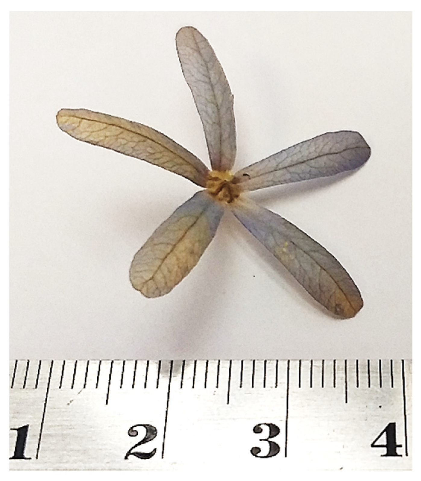
Some of the most known biomimetic wind turbines are the Maple and Dryopbalanops Aromatic seeds. Like the Petrea Volubilis so-called Machiguá flower shown in Figure 1, the seeds have special behavior which consists of a free vertical rotation as they fall from the tree branch; this motion is so-called autorotation. This behavior makes those seeds suitable to mimic the designing of wind turbines, hence it is expected that this attribute could be used to transform the kinetic wind energy into mechanical energy efficiently. From the Maple seed, physical characteristics were determined experimentally and then compared to numerical simulations [11], deploying good potential for wind turbine design. The Dryopbalanops Aromatic seed was simulated by OpenFOAM and compared to a three-bladed HAWT to determine the accuracy in predicting rotor performance [12].

Designing with CFD simulations is one of the most employed techniques [13], but is still noted that BEM has high advantages in contrast with CFD predictions; in this case, BEM saves computational resources while retaining the accuracy of calculation. This is a great advantage in wind rotor engineering applications. On the other hand, CFD also has advantages over BEM for new designs, one of them is that CFD captures the real unsteady behavior of flow over the blade. But by taking into account new theories, BEM has high potential, some of the new theories adapted by BEM give extremely efficient and accurate results in comparison with CFD. In this sense, those techniques may be complementary to one another [14]. Reduced-order methods have been developed to make this process more agile while keeping the complexities of the flow; some of these techniques are Actuator Disk and Actuator Line models to solve the Navier–Stokes equations, employed with success in the investigation done by Matiz and Lopez [15], other related techniques are those called the vortex or lattice methods.

An approach to experimentation adapting Petrea Volubilis as a wind rotor design was done for the first time by Catañeda [16]; this seed consists of five equiangular petals, shown in Figure 1, and those petals are considered as blades of a wind turbine during the simulation. The petals are slightly tilted backward. Once the seed falls from the tree, the branch has, in general, 3.5 to 5 cm diameter; each blade is cambered along chord and radial axis, as simple inspection may show.

Nevertheless, for Petrea Volubilis rotor to compute aerodynamic coefficients is a challenging process since numerical methods and turbulence models have to simulate the real flow behavior and additionally there is a huge computing time involved to solve the governing equations in big meshes associated with big rotors while capturing the effect of the tridimensional nature of the flow around the tip.

The power performance for the biomimetic wind rotor is the aim of the present study, it is presented an experimental procedure and a CFD simulation of a wind turbine inspired by the seed Petrea Volubilis, also known as Queen’s wreath or Machiguá flower found in Cordoba, Colombia. The results obtained are compared to experimental data to validate the results obtained. Simulations and mesh generation were performed by the open-source code OpenFOAM. Results showed good agreement between simulations and experimental data and it was concluded that from 4.5 up to 6 m/s is an operative flow range speed, on which this rotor has its maximum operative performance.

This paper consists of this introduction part, Section 1, showing an experimental set up with a detailed experimental arrangement. Computational simulations configurations, computational code description, meshing process, and computational set-up are presented in Section 2. In Section 3, the results and discussions are shown. Lastly, Section 4 contains conclusions and further work.

2. Experiment Set-Up

In order to compare experimental data and CFD results, there have been used Machiguá similar biomimetic rotor parameters as Castañeda [16] and Wahanik [17] did. Rotor blade parameters are: a constant thickness overall rotor blade shape; the roughness is according to that obtained with a 1000 sandpaper over gel coat resin; the blades are independent of the hub for experimentation; those rotor blades can rotate in a radial axis.

Three non-dimensional parameters were used for experimentation. These equations relate to the torque produced by Machigua’s wind rotor as well as rotor wind and rotational speed. The torque coefficient $\left(C_{\tau }\right)$ was used for the torque measured. The power coefficient (${\mathrm{C}}_{\mathrm{p}}$) in Equation (1) also was used in the experimentation; ${\mathrm{C}}_{\mathrm{p}}$ is used along within this study to measure the performance of the wind turbine. Tip Speed Ratio λ also referred to (TSR) was used to take the non-dimensional the rotational parameter of the wind rotor. Non-dimensional coefficients used in the experimentation are presented in Equation (1) through Equation (3).

$${\mathrm{C}}_{\mathrm{p}}=\frac{\tau \ast \omega }{\frac{1}{2}\ast \rho \ast V_{wind}^3\ast A}=\frac{P_{extracted}}{P_{avaliable}}$$

(1)

$$C_{\tau }=\frac{\tau }{\frac{1}{2}\ast \rho \ast V_{wind}^2\ast A}$$

(2)

$$\mathsf{\lambda }=\frac{\omega \ast r}{V_{wind}}$$

(3)

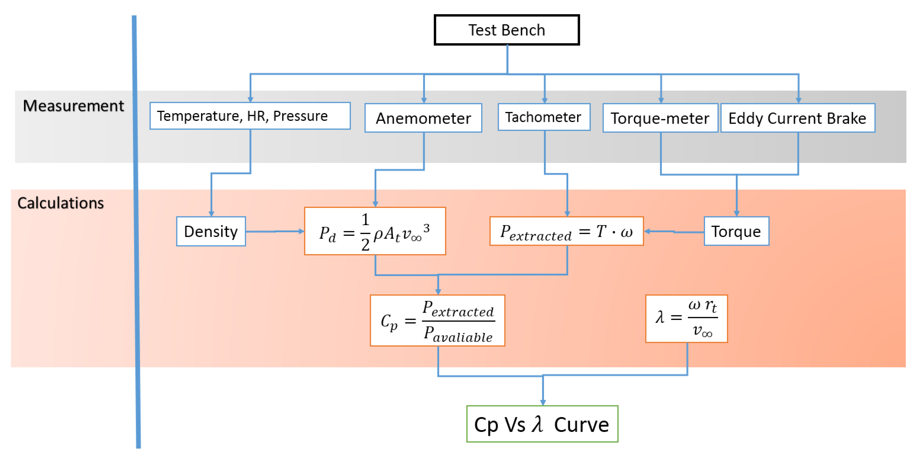
With respect to those equations, experiments were configured according to the following methodological scheme (Figure 2). The Cp vs λ curve was constructed according to the measurement devices that are considered in this figure. To measure density the following sensors devices have been used: temperature, air humidity, atmospheric pressure sensors. Available power has been measured with an anemometer device and the density already calculated. Extracted rotor power has been measured with a tachometer and an inline torque meter. The inline rotor shaft torque metering device was supported with an Eddy Current Brake system (Foucault brake).

In Figure 2 and in Equation (1) through Equation (3) there are the following variables:

-

$P_d$ is the available power;

-

$\rho$ is the environmental density;

-

$A_t$ is the wind rotor front projected area;

-

$v_{\infty }$ is the up-stream velocity;

-

$T$ is the rotor shaft torque;

-

$\omega$ is the rotor angular velocity;

-

${\mathrm{C}}_{\mathrm{P}}$ is the power coefficient;

-

$P_e$ is the extracted power from rotor, also referred as $P_{extracted};$

-

$P_a$ is the available power, also referred as $P_{avaliable}$;

-

$r_t$ is the wind rotor radio;

-

$\mathsf{\lambda }$ is the Tips Speed Ratio (TSR).

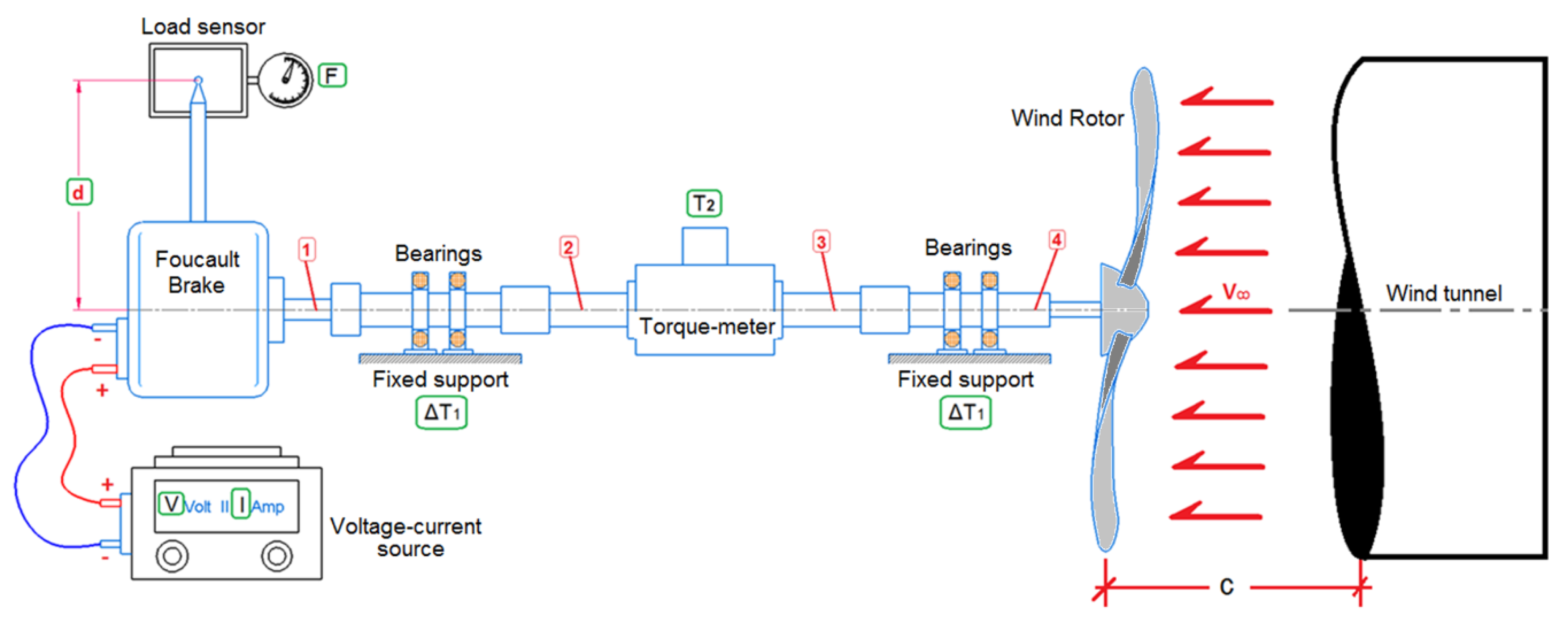
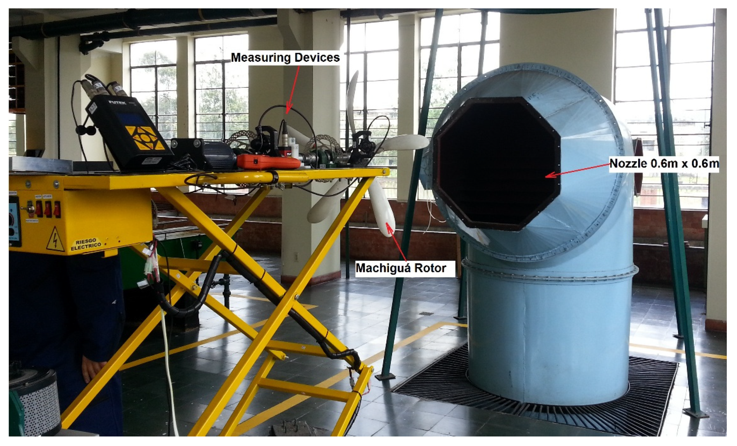
5 blades for Machigua’s seed rotor was used along with the experimentation. Rotor diameter in experimentation was 0.6-meter diameter, as well as the computational configuration. A free rotation (no brake applied) speed range was measured from 180 to 1100 Rpm for an upstream velocity range from 4 to 14 m/s. The experimentation was configured with a variable pitch rotor blade angle. This angle was used for all blades (refer to Figure 4). Machigua’s seed rotor blades were made of fiberglass covered with a white Geal Coat. Those blades were placed in position using conical gears. The distance from the rotor to the nozzle was 1.8 meters (distance c with respect Figure 3 and Figure 5). The nozzle had a maximum cross section of 0.6 × 0.6 m.

Relative to the scheme in Figure 3 and Figure 4, an in-line torque-meter was used to calculate supports bearing frictional losses. In-line torque meter range is up to 3 Nm with an accuracy of 0.2%. A barometric pressure/relative humidity and temperature device sensor was used to measure density, a barometer with a resolution of 0.1 hPa was used, and a relative humidity sensor was also used; this barometer has an accuracy of 4% and the temperature sensor has an accuracy of 0.8 °C. The tachometer used had a resolution of 0.1 rpm. A Foucault brake was also used, which had an operating range of up to 1800 RPM, 24 Volt, and 1 Ampere as maximum operating conditions. A hot wire thermo-anemometer sensor was used to measure both $v_{\infty }$ and upstream temperature; this anemometer had a resolution of 0.01 m/s.

According to Figure 3 power in point 4 is the power given by Machigua’s wind rotor to the shaft. Power on the wind rotor axis (point 4 of Figure 3) is calculated from Foucault brake and in-line torque-meter. Bearing frictional losses are measured using the in-line torque meter. Taking into account the bearings friction losses, power is calculated as

$$P_4=P_m+2\ast \Delta P_1=P_2+\Delta P_1$$

(4)

where Pm is the mechanical power in point 1.

According to Figure 3, losses in the supports can be calculated as

$$\Delta P_1=P_2-P_1$$

(5)

where: $P_2$ is the power measured in the in-line torque-meter; $P_1$ is

$$P_1=P_{\mathrm{m}}=F\ast d\ast \omega$$

(6)

Here, F is the force measured by load sensor; “d” is the distance from rotational axis to load sensor.

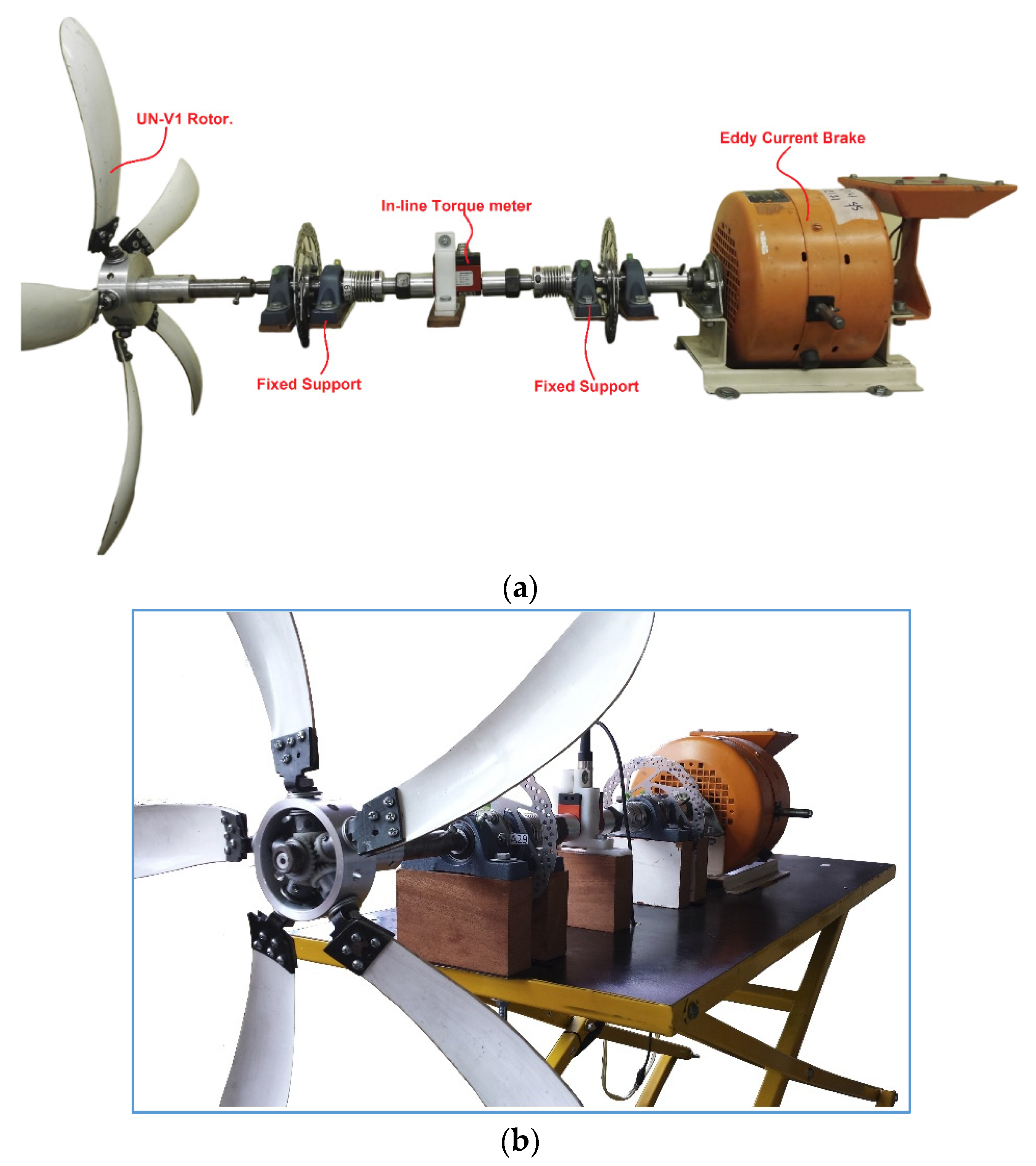
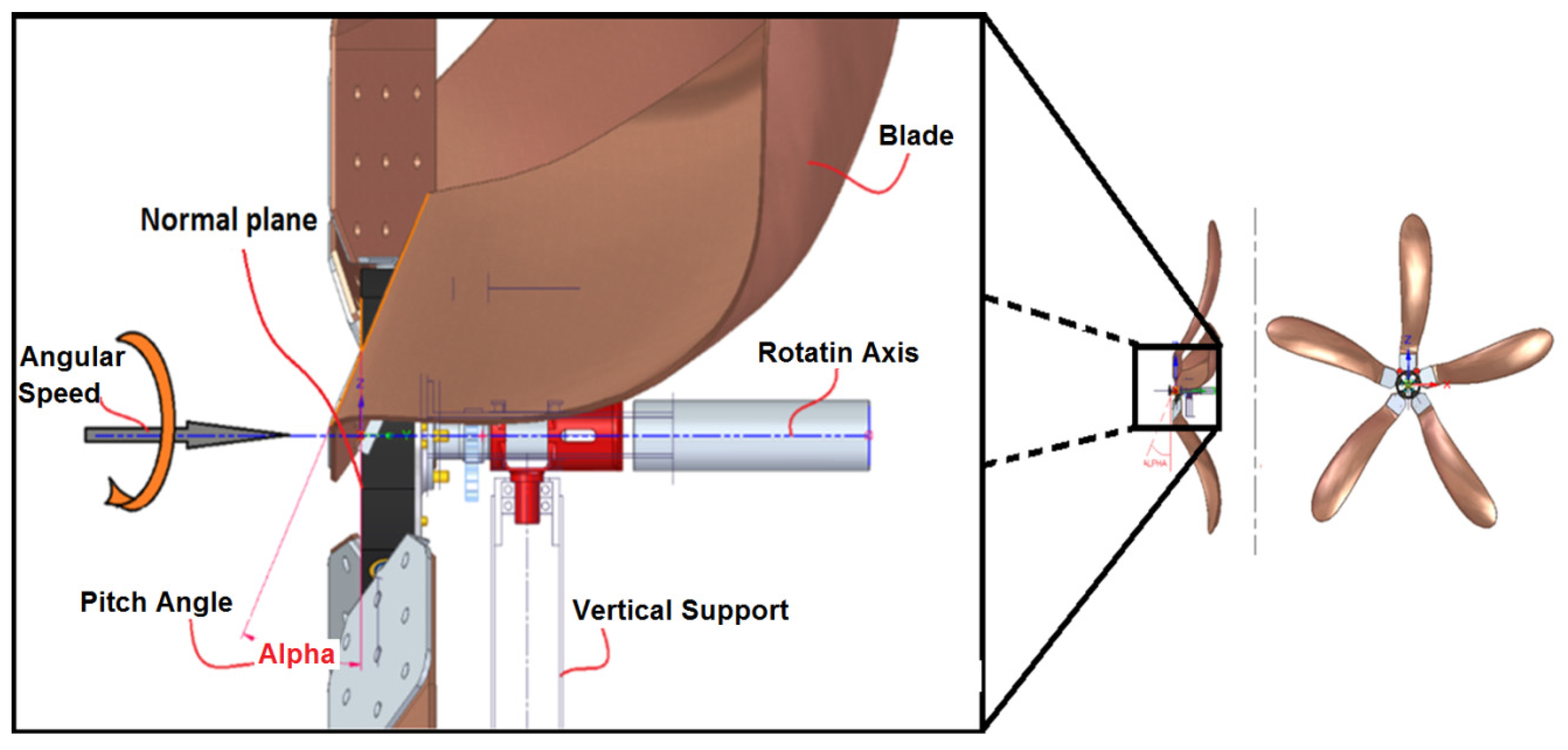
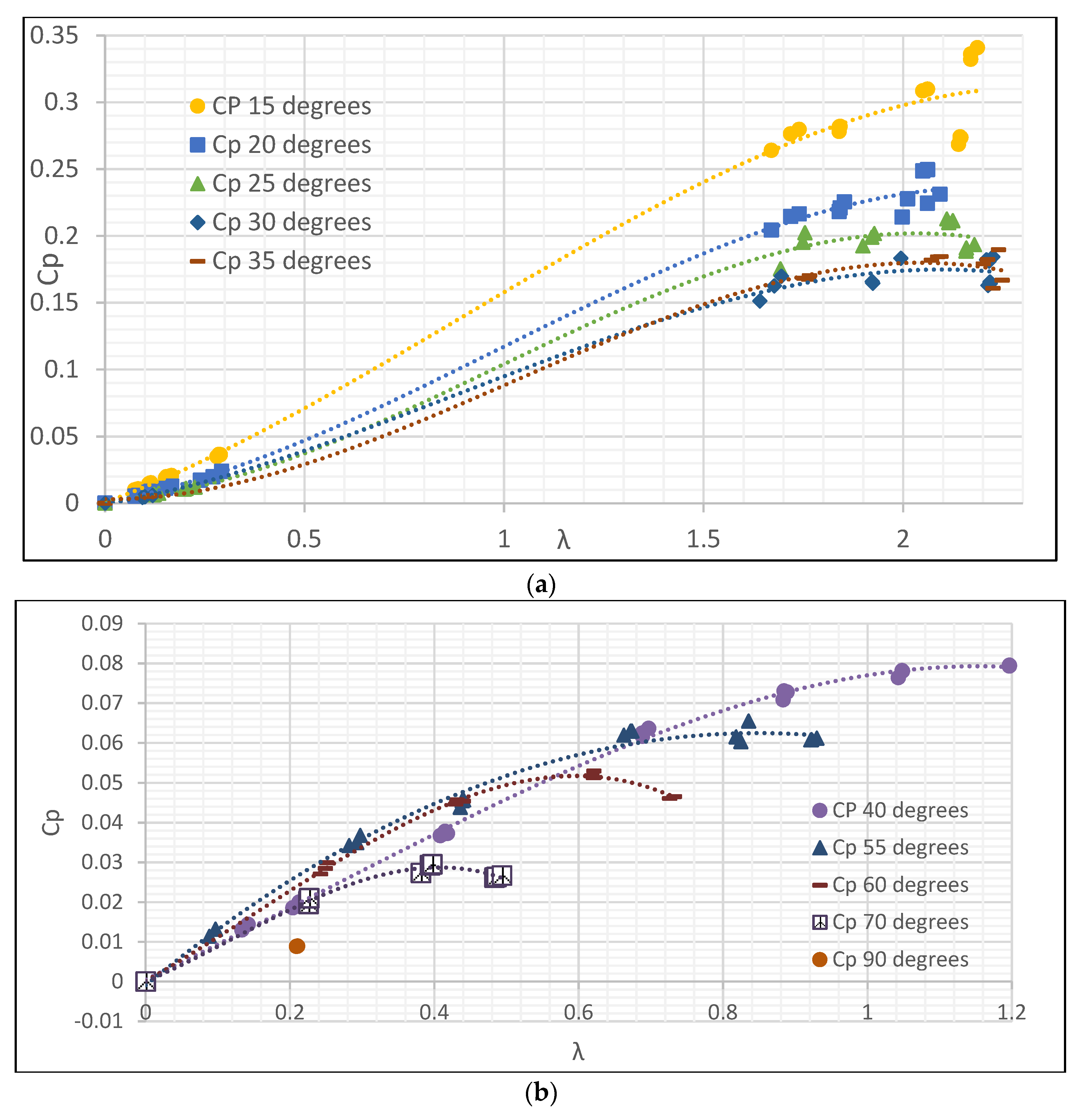
The complete arrangement of the test bench with the measuring devices is shown in Figure 4 and Figure 5. Along with the complete experimentation, a variable blade pitch angle was configured, which was able to test each angle. A total of six pitch angles were tested in this investigation. The pitch angle range was from 15° to 75°.

3. Computational Set-Up

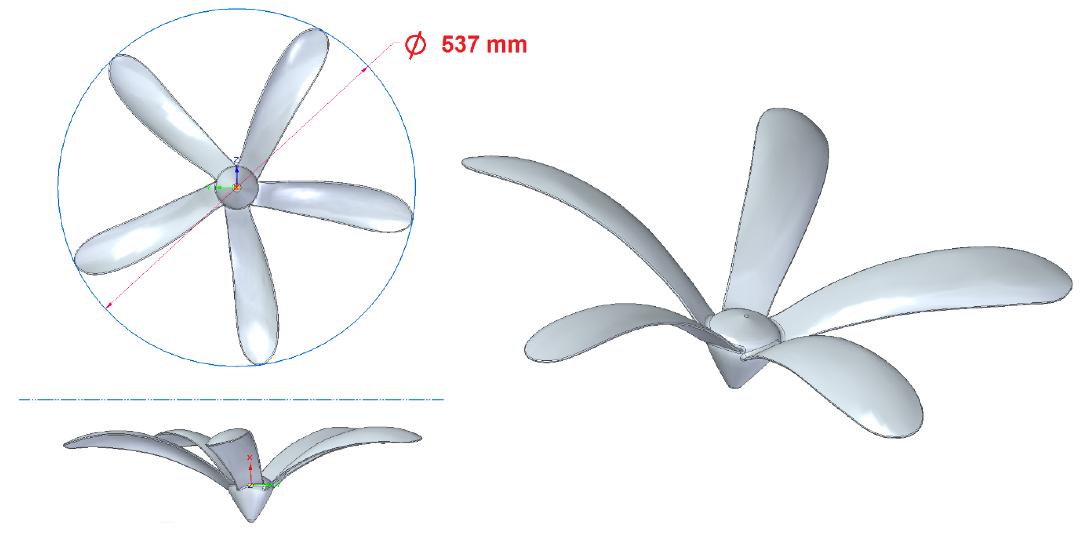
To perform the simulation, the Machiguá’s seed was scaled up to 0.537 m diameter to compare the results with respect to those given by Castañeda and Wahanik [16,17] who did an experimental and computational approach for this biomimetic rotor using hydraulic brake system for experiments and RANS as turbulence model based on Ansys Fluent software for CFD analysis. 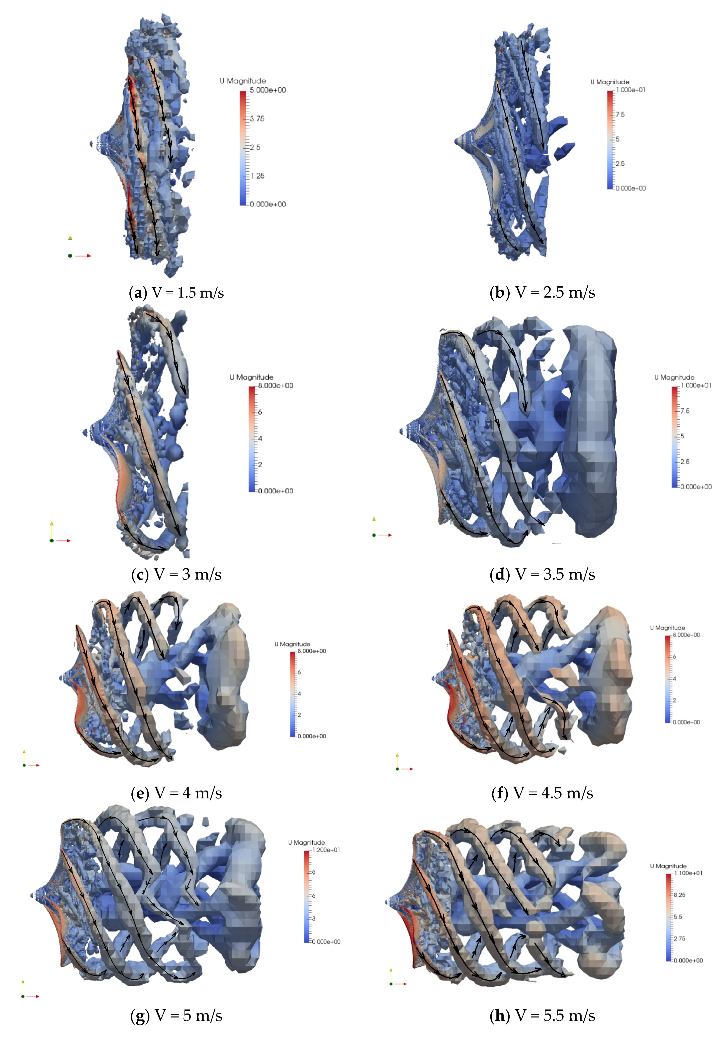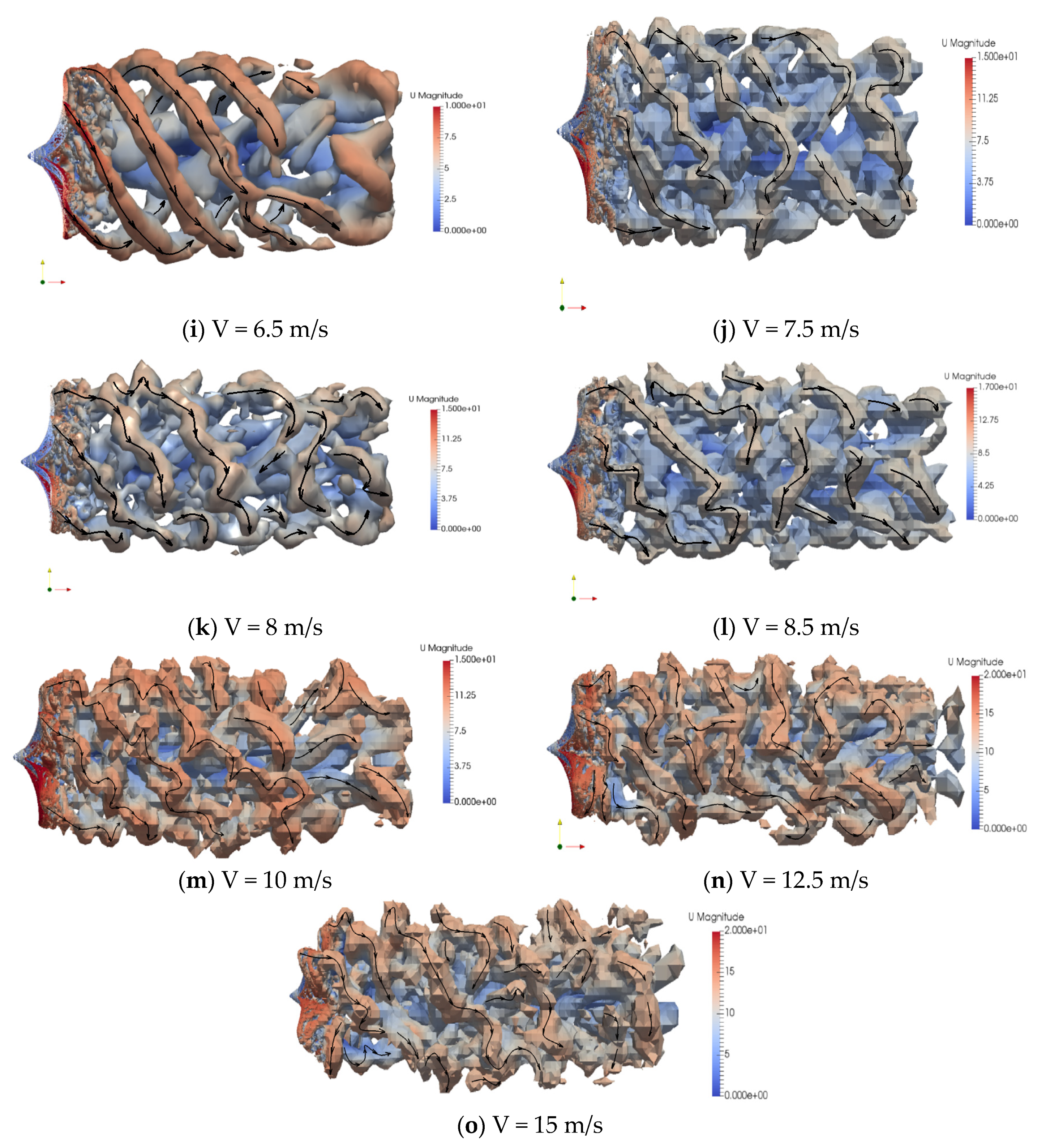During the simulation the blades were configured at a constant 15 degrees pitch angle, this angle is measured based on Figure 6. Simulations of the biomimetic wind turbine with five petal/blades were performed at a range of 1.5 up to 15 m/s wind speed and a rotational velocity of 312.5 rpm.

Computational simulations were performed with the open-source code OpenFOAM 3.0+ version, a free-licensed software used to solve the governing equations of fluid dynamics so-called Navier-Stokes Equations based on the finite volume method (FVM). The operative system used was Ubuntu 14.5.

Turbulence modeling has always been a key issue to solve when using CFD methods. There are four common ways to achieve turbulence modeling: Reynolds-Averaged Navier-Stokes (RANS), Large-Eddy Simulations (LES), Direct Numerical Simulations (DNS) and hybrid methods that combine RANS and LES (DES). RANS has been the most used method due to that it requires the less computational resources achieving acceptable results; however, LES has become a powerful tool and its application is now more often in engineering problems even though it requires high computational resources. The high computational cost of LES is due to that solves large and small turbulent scales; this is done by solving the largest scales over a generally coarse mesh by computing the exact solution and to model the smallest scale by using a sub-grid scale (SGS) model [18].

The Machigua seed simulations were performed by employing incompressible LES turbulence models with a localized SGS dynamic one-equation eddy-viscosity, this model was proposed by Kim and Menon and it couples the dynamic behavior of the SGS model introduced by Germano et al. [19] with a transport equation for the SGS kinetic energy (ksgs). This model provides one kinetic energy equation closure in which the model coefficient does not remain constant rather it is determined as part of the solution, having two positive outcomes: first, it models more accurately the sub-grid stresses in different types of turbulent flows; second, the coefficient can eventually become a negative value in certain regions hence it has the capability to mimic the deflect energy behavior from the smallest to the largest scales [19]. Computing the kinetic energy (as shown in Equation (7)) allows the model to take into account the details of the flow structure and the turbulence development history [20] computing the SGS eddy viscosity (μ_t) as shown in Equation (8).

$$k_{sgs}=\frac{1}{2}\left(\overline{u_k^2}-{\overline{u_k}}^2\right)$$

(7)

where, $\overline{u_k^2}-{\overline{u_k}}^2$ represents the fluctuation of the velocity field in a resolvable scale,

$${\mu }_t=C_k{k}_{sgs}^{1/2}\Delta$$

(8)

where C_k is a dynamic coefficient calculated by filtering the velocity field, and ∆ is the width of the spatial filter, typically related to grid resolution.

Additionally, this model avoids numerical instability, common in other dynamic methods, by doing a spatial averaging in terms of vorticity associated with the transport equation rather than homogeneity flow directions, common in other dynamic coefficient methods.

3.1. Computational Domain and Meshing

The main dimensions of the computational domain are related to the seed dimensions taken in the experimentation and simulations given by Castañeda and Wahanik [16,17]. They kept the same rotor size for both experimentation and numerical simulations. Rotor’s diameter shown in Figure 7 is 0.537 m. To obtain similarity between the simulation and the original design it was modeled the hub. The blade has a constant 2 mm thickness over all the blade radius.

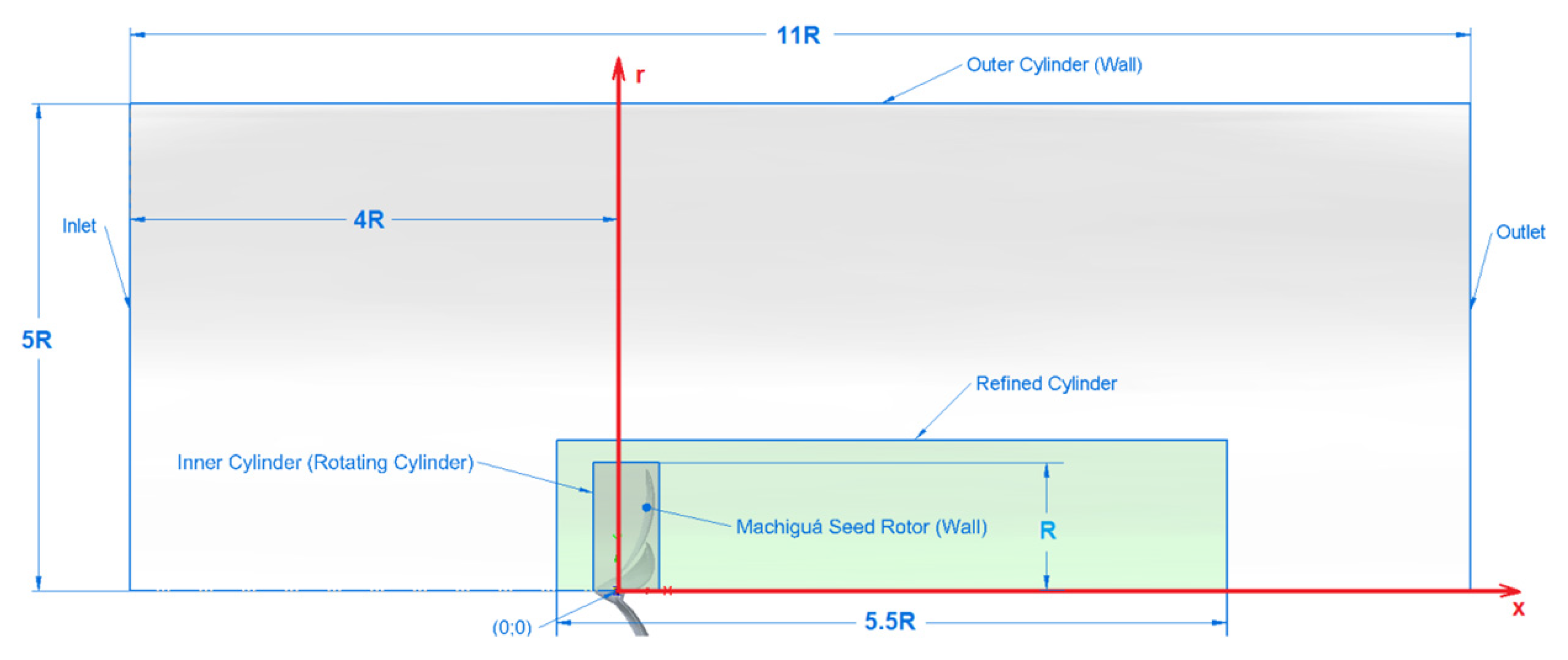
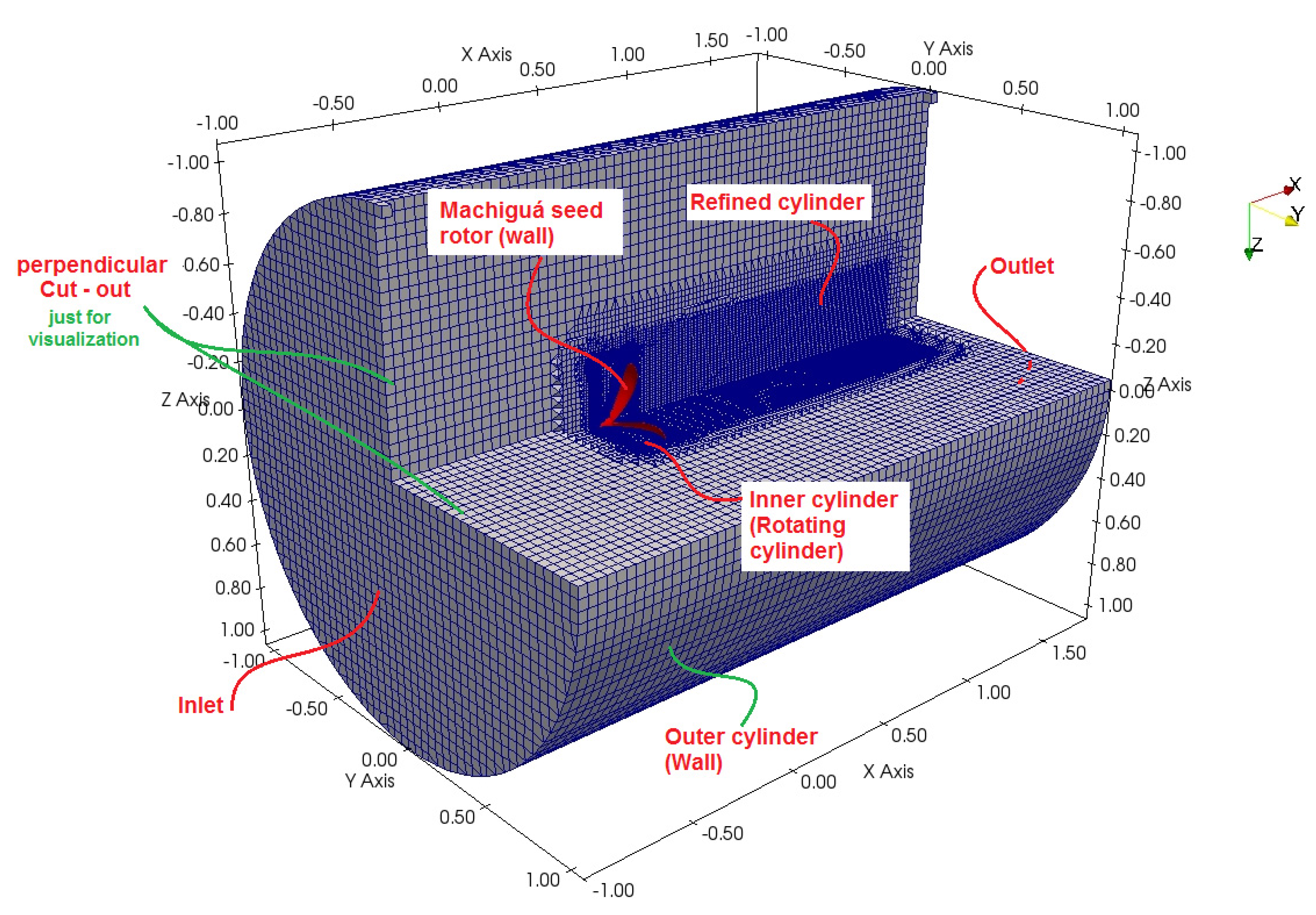
The geometry of this domain was established as a cylindrical form. The overall dimensions of the computational domain considering the center axis inside the rotor were determined in terms of the rotor radius (R) as: 4R forward, 7R backward and 5R side. The structure of the domain was established taking into account the boundaries as shown in Figure 8 [21,22]. There were created 3 zones to perform the simulations:

• An inner cylinder was configured to rotate during the numerical simulation. The boundary for this area has an Arbitrary Mesh Interface (AMI), on which two meshes are placed simultaneously: a mesh fixed in the external computational domain and a slave mesh attached to the rotating area. On this dynamic mesh was placed the rotor;
• A refined cylinder was created to take a detailed visualization of the vortex generation downstream of the rotor;
• Lastly, the perimeter lateral boundary for the outer cylinder is considered as a wall during the computational simulations.

Configuration of the mesh was based on a primary blockMesh dictionary of OpenFOAM. A general block was configured with a mesh size of 60, 50 and 50 cell along the x, y and z-axis, respectively. The general block has a square cross-section of 2.8 m length and 3.2 m depth. The outer cylinder has a refinement order concerning the initial blockMesh configuration of 1. The inner cylinder has four orders of refinement and the zone called refined cylinder has 2 orders of refinement. Each boundary was established with an expansion factor of 4 concerning its neighbor zone. Also, each boundary was set up with an individual refinement level. For the inner cylinder, a refinement level ranging between 3 and 4 were used and 5 to 6 for the rotor.

A wall stress function based on Von Karman’s work was considered for the rotor [23]. To take into account the boundary layer it was needed to establish the predominant turbulence level as well as the turbulence model [24]. To consider the boundary layer, a predominant mean Reynolds number of $230\times {10}^3$ was analyzed. To do this, it was considered an angular velocity of 32.73 rad/s. Air dynamic viscosity based on a temperature of 20 °C was applied to the Reynolds number. A Shlinchting Friction wall coefficient approximation was used based on predominant Reynolds number as it is shown in Equation (9). This coefficient was used to establish a wall shear stress. A value of τ_w = 0.194 Pa was calculated giving a friction velocity of 0.46 m/s.

$$C_f=0.0592{\mathrm{R}}^{-1/5}=5.7\times {10}^{-3}$$

(9)

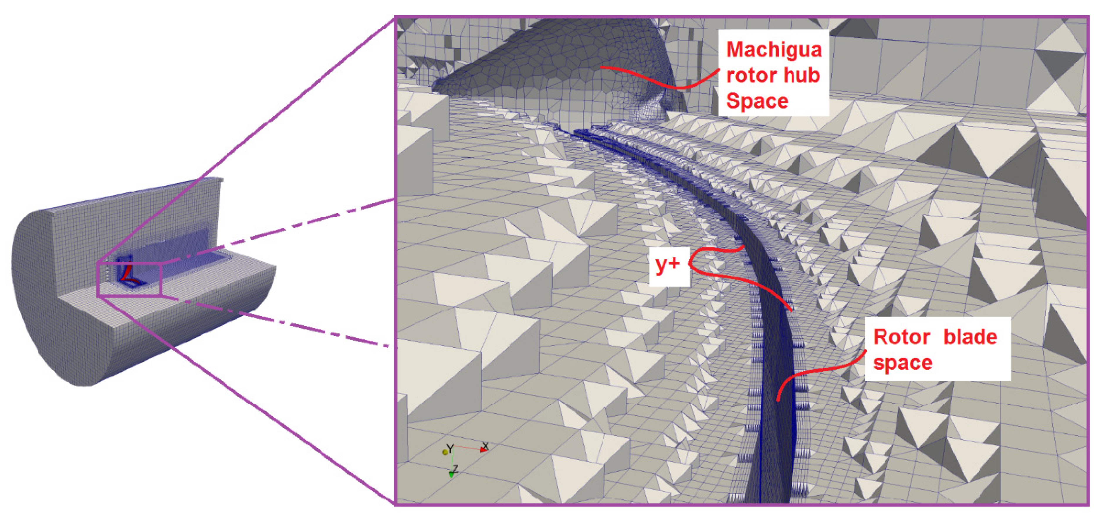
The One Eddy Equation (Large Eddy Simulation) was employed as a turbulence model. To consider the boundary layer under the LES turbulence model it was considered a y⁺ = 1 as equivalent wall distance [22]. The first cell of the boundary layer was calculated as shown in Equation (10).

$$y=\frac{\mu ·y^{+}}{\rho ·U_T}=4.32\times {10}^{-2}\mathrm{mm}$$

(10)

The size of the first cell from the rotor’s wall (y) was considered as 0.04 mm. From the boundary layer, six cells were set over the rotor and an expansion ratio of 1.1 was applied for this boundary cells [22]. The outer cylinder was not considered a wall stress function of the mesh. The full mesh is as shown Figure 9 and Figure 10.

An arbitrary mesh interface (AMI) was employed as an interphase to communicate information between the rotational part with the Machiguá’s wind rotor and the outer mesh. Inner cylinder zone was set to rotate at a constant angular velocity of 32.73 rev/s with respect to the center x axis of the full computational domain shown in Figure 8.

3.2. Solver

The open-source code OpenFOAM version 3.0 was used to perform all simulations of the present study. The governing equations for incompressible flow: continuity and momentum conservation, were solved using a segregated pressure based on PIMPLE solver. Pressure-linked solver equations are basically two: Semi-implicit method for pressure linked equations SIMPLE is a steady-state solver for incompressible flow that solves the discretized momentum equations to compute a “virtual” velocity field, hence the mass fluxes at the cell faces and finally solve the pressure equation which is used to correct the mass fluxes hence to correct the velocity field in an iterative process until convergence [25]. An extension of this algorithm for unsteady flows is implemented, Pressure Implicit with Splitting of Operator—PISO differs from the previous algorithm by repeating the process above and in the end increases the time step to solve again the momentum equation then it also advances through the time. The PIMPLE solver employed in this work merges the SIMPLE and PISO algorithms. For the time dependent problem it was established variable time-step to follow the rule Courant number less than 0.95 to keep stability and reduce the computational time.

The discretization of the governing equations was done by an interpolation scheme derived from the linear-upwind algorithm which returns blended linear interpolation with linear-upwind weighting factors and applies a gradient-based correction obtained from the linear-upwind scheme. In this way stability of solution is handled maintaining second order behavior. This scheme, Linear-Upwind Stabilized Transport (LUST) is used particularly in simulation of complex geometries and external flow applications [26] and was employed to discretize the convective term; for the turbulent kinetic energy was employed a Gauss-based interpolation and time was discretized by a second order backward scheme.

4. Results and Discussion

4.1. Experimental Results

The results of the torque were based on a variable blade pitch angle from 15 to 35 degrees. Results are shown in Figure 11, a total of nine variable blade pitch angles were tested, and different behavior was noticed along with the results:

a-

Maximum value was for pitch blade of 15° with a mean value of 0.32 in Cp and a Cp value of 0.18 for 35°, pitch angles higher than 35° has a considerably lower Cp maximum value, from Cp = 0.07 for pitch angle of 40° up to Cp = 0.02 for pitch angle of 70°.

b-

Two groups of blade pitch performance can be observed in Figure 10a,b. A group from 15° to 35° where there is a quasi-similar maximum Cp value for λ ≈ 2. The second group from 40° to 90° (rotor Blade pitch angle) with a considerably lower maximum Cp value compared with the previously described group. It is noted that for an increasing value in blade pitch angle there is a decreasing value for maximum measured Cp Value.

c-

For the first group, there were observed that there are no measured points in λ range from 0.3 to 1.6. This occurs due to a sudden change in angular velocity for a short change in $v_{\infty }$, a representative example for this behavior is shown in Figure 12, in this figure it is evident two sections: before point A and after point B. In the first section, there is an increasing angular velocity and a quasi-lineal behavior for both angular velocity and torque, the rate of change for torque and angular velocity is 1/10 and 1/16.5 respectively. The second section occurs almost sudden, 0.8 m/s after A point, in this section can be measured its initial slope to check the local rate of change and there is measured initial slope for torque and angular velocity as 1/6 and 1/4.5 respectively.

Comparing slopes for angular velocity (1/16.5 before point A and 1/4.5 after point B) is notable that this sudden behavior affects the Cp curve for Figure 12 making no measured points in the related λ range. This sudden behavior was observed for all rotor blade pitch angle measured shown in Figure 12a.

For the Cp Curve, it is noticed that the maximum Cp is obtained for a rotor blade pitch angle of 15° and this angle is the angle analyzed in CFD.

4.2. Computational Results of Torque

To ensure results independency from the size of the mesh a study of grid independence was performed, the parameters at which the study was completed are 5 m/s wind speed, 310 RPM as angular velocity. The number of elements in each mesh was set from $1.99\times {10}^6$ to $4.4\times {10}^6$ cells. One equation Eddy (LES) turbulence model was used. The results of those analyses are as shown in Figure 13.

A stabilizing mean value for the x-moment was evident with a mesh of $2.8\times {10}^6$ cells and 0.1585 N*m as shown in Figure 13. Therefore, this mesh was chose to perform the simulations and computational analysis.

At 15 degrees pitch angle results for different airflow velocity shows a quasi-proportional increasing of the rotor torque. Figure 14 shows how extracted power has a variable increasing rate meanwhile airflow speed increases. Figure 15 shown values for Cp vs TSR. Three relevant aspects can be analyzed from those figures:

• A initial increasing power starts from 1.5 m/s up to 5.5 m/s (Figure 14), in that range, the maximum Cp is located at 4 m/s whose corresponds to a TSR of 1.94 with a Cp = 0.429 (Figure 15).
• There is a transition range between 6.5 m/s to 8 m/s on which there is located the maximum slope of the Cp curve, this range match with a TSR range from 1.03 to 1.25. In Figure 14 there is a decrease in the rate of change from 6.5 m/s up to 8.5 m/s whose corresponds to a λ value of 1.34 and 1.03 respectively this variation in torque rate of change corresponds to the highest rate of change in Cp curve, in this curve at the same λ range there is located the inflection point.
• A range speed from 8.5 m/s to 15 m/s corresponds to initial section of the Cp curve with TSR from 0.58 to 1.03.

In Figure 14 there is a velocity on which the power is zero, from this point power begins to increase power for an increase in upstream velocity, it is evident for CFD prediction that there is not or negative power for velocities lower than 2.5 m/s, this behavior suggests that the start wind speed for Machigua rotor is 2.5 m/s. Comparing this behavior with Cp curve (Figure 15) it is shown that when power is positive there a higher increase in power reaching faster to maximum Cp for small values of airspeed. With the power curve and Cp curve predicted by CFD is noted that Machigua rotor can produce faster a maximum power with a lower rate of change of velocity.

Curves on Figure 15 corresponds to Cp vs λ, Power vs λ and a derivative curve of Cp respect to λ. The derivative curve shows inflection and maximum points of the Cp curve. Inflection of Cp is located at the maximum section of the derivative curve with λ of 1.09 on which the power curve has local variation for the range related in numeral 2 “experimentation set-up” explained above. Inflection point has a Cp value of 0.2 at 1.09 for λ. It gives 10.47 watt power at 8 m/s. Maximum Cp corresponds to 0.42 at 1.94 λ. Maximum Cp is obtained with 3.92 Watt at 4.5 m/s.

Ct vs λ curve shown in Figure 16 has its maximum value at 1.59 λ with Ct at 0.065. This value do not necessary match with maximum value for Cp vs λ. Torque curve increases for a decrement on λ value when angular speed is constant. Maximum value for torque is 0.626 at λ equal to 0.58, and it has its minimum torque value 0.04 at λ equal to 3.5. At maximum Ct curve Value Cp is equal to 0.387. It is a 9.79% less than its maximum Cp value. According to Van Meel & Smulders maximum value for Ct in new wind turbines must be under 0.2.

Simulation results for Machigua (Petrea Volubilis) biomimetic rotor predict its fluid dynamic performance for this scaled rotor. In order to compare results in the Figure 17 results is presented the Machigua seed results from Castañeda (experimental) and CFD from Wahanik. LES turbulence model computational results can be compared in respect of those experimental ones. Experimentation on both works was performed similarly in rotor size. Figure 17 shows performance curves for experimentation and for LES numerical simulations. In Figure 18 there is included a comparative biomimetic rotor called Dryobalanops aromatica seed presented by Yung-Jeh and Wen-Tong [13]. They studied a biomimetic rotor performance with 3 blades with variable blade pitch angle and this rotor is compared with Machigua seed.

As power extraction is one of the most determining parameters in rotor performance there was analyzed 15° as the pitch angle with the maximum Cp value, the pitch angle was measured as shown in Figure 6. Machigua rotor blades has a constant thickness and there has not been changed rotor blade parameters like cross-section profile or twist angle. The blade cross-section and the local twist angle disposition, as well as consideration to improve profile with an aerodynamic NACA one, will be conducted for future works.

The simulation results show that the biomimetic Machigua wind rotor achieved maximum value at Cp = 0.429 at λ = 1.94. Experimentation (both Castañeda and current study) gave a remarkable group range results for λ from 1.7 up to 2.6. This range matches with maximum Cp for CFD and experimentation. In experimentation, the maximum Cp range is between 0.3 and 0.36. The maximum results for LES simulation have the same λ range than experimental values. The difference between experimentation and LES simulations has 21%. A comparison between the current CFD study and Wahanik results show a similar maximum power coefficient values with a difference of 3.54% but at different values for λ. The maximum Cp value for Wahanik occurs at λ = 2.65 in comparison with the current study Cp maximum occurs at λ = 1.94. It is noted that the Wahanik Cp curve tendency almost matches with the current study curve but with a λ offset of 0.707 (26.66%). There is a similar behavior for Cp from experimentation given by Castañeda and the current study, Castañeda did a Cp measurement with a hydraulic brake by varying the pressure around a disk connected to the rotor shaft, meanwhile, the current study used an in-line torque meter.

Comparative results for experimentation shows a remarkable range on which the Cp values for Castañeda respect to the current study match; over this range (1.86 < λ < 2.26) experimental results coincide with a wide range for Cp results along with curve results. These experimentations are complementary for comparison purposes, the lowest values of λ shows small linearity in Cp response, this behavior is for upstream velocities from 11.1 m/s up to 13.5 m/s. for λ values higher than 2.26 Castañeda experimental Cp values decrease at a mean rate of –1/3.3.

The difference between CFD and experimental results for Machigua rotor is based on the measuring device for experimentation who has not been considered for CFD. The measuring devices affect considerably the vortex downstream of the rotor (consider rotor vortexes in Figure 21). Vortexes behavior in the simulation are not affected due to there is no system similar to a measuring device. As velocity values for experimentation decrease meanwhile λ increases, there is a range on which the experimentation has no results. Non-comparable values are shown in the λ range of 0.5 < λ < 2.

Performance parameters for Petrea Volubilis and Dryobalanops aromatic [13] wind rotors results are presented in Figure 18, the highest experimental Cp values from various rotor blade pitch angles are presented in this figure 10°, 15° and 20°, in the original seed shape it has 5 blades or petals, a rotor model proposed based on this biomimetic seed was analyzed by Yung-Jeh and Wen-Tong. It is evident that the Dryobalanops rotor compared with the Petrea rotor has maximum value for Cp is almost the same value on the 10^o pitch angle (Cp = 0.39 for Dryobalanops), a mean difference for this pitch angle is around 7.42% compared with Petrea rotor. Values for maximum Cp on Dryobalanops occur at λ = 1.5 meanwhile the maximum Cp for Petrea is located at λ = 2. The maximum Cp value for 20° and 10° for Dryobalanops is 0.38 whose is higher than the maximum Cp value for Petrea, the difference between both maximum values is 16.1%.

This small difference between those biomimetic rotors remarks similar performance for both biomimetic rotor designs. On both designs, there have been used cross-section profile just considering a constant thickness over all the rotor blades. There are considerable advantages from one rotor to others.

Comparable CFD power results are shown in Figure 19, comparable results with respect to those in Castañeda experimentation coincide from 4.58 m/s (4.04 Watt) and 5.06 m/s (5.47 Watt) where the power difference is 2.78% and 5.3% respectively. From velocities higher than 5.31 m/s power values differs from CFD results in 6.45% where experimentation power value is 5.59 Watt and CFD value is 5.97 Watt. The difference between Castañeda experimentation results and CFD prediction increases as $v_{\infty }$ increases, the higher difference on both results corresponds to $v_{\infty }$ of 7.5 m/s where a difference of 10.41% is measured. There is a difference in the rate of change of power to $v_{\infty }$ in the velocity range of 5.38 < $v_{\infty }$ < 7.44, where CFD results have a rate of change of 1.65 for Castañeda experimentation and 1.95 for CFD results.

It is also presented in Figure 19 a comparison between CFD and experimentation results from the current study. For $v_{\infty }$ range from 11.1 m/s up to 13.5 m/s it is only comparable CFD power tendency curve and experimentation power curves, it may be noted a similar slope curve from CFD and experimental results on which for CFD there is a mean slope is 1.65 meanwhile for experimentation there is a mean curve slope of 1.97. A difference in slope power curves of 16.24% has also power differences for velocity in 11.1 m/s and at 13.5 m/s. The experimentation compared to a linear extrapolation for this velocity range in CFD prediction gives a difference of 13.9% for power points in 11.1 m/s on both results and a difference of 6.15% in 13.5 m/s.

4.3. Vortex Structure

Tip Vortexes are formed at the blade rotor tip toward downstream, those tip rotary vortexes extend downstream at a maximum distance of 6R where those vortexes begin to dissipate. Figure 20 shows an example for vortex structure at a side view for this rotor, here it is shown a detail at the closest view projected from the axis longitudinal rotor line. As it is shown for each individual vortex there are at least 3 vortex components, axial, tangential and radial vortex components. In Figure 20 there is only shown axial and tangential components.

Different upstream velocities produce different vortex components, some of those velocities generates a higher axial component than tangential component, this behavior is present in Figure 21 where the vortexes has been filtered. Vortex visualization is achieved using the second invariant (Q) of velocity gradient tensor ($\nabla$u) under the Q-Criterion. Here those values must be positive (Q > 0). In Figure 21. Q value is inside the range 200–250; here there is evident the representation of the local balance between the shear deformation rate and the velocity magnitude where those visible vortexes are fluid regions on which the velocity magnitude is higher than the deformation rate magnitude [27].

Figure 21 shows the vortexes structures and it is also shown a representative vector indicating the predominant direction for vortexes meanwhile are moving downstream the flow. There is also shown the vortex behavior for a velocity range from 1.5m/s up to 15 m/s. There are two groups vortex behavior and they have been divided taking into account the θ angle shown in Figure 20. For a velocity range between [1.5 m/s and 6.5 m/s] the measured angle has the range [62°–77°] and it is noticed the positive (downstream) component for axial vortexes flow. Also, it is notable that for lower velocity (6.5 m/s) there corresponds to an angle of θ = 77°. In general, for upstream velocities below 6.5 m/s there are always positive vortex axial flow components.

For upstream velocities higher than 6.5 m/s, there is an increasing range for θ; chaotic vortex structures give values for θ greater than 77° in various flow fields. This behavior gives, in many cases, negative components for vortex axial flow, and a considerable turbulent zone is present. This also brings a decrease in the power of velocity flow, due to a sudden rapid change in velocity direction. This process takes a considerable amount of flow energy and consequently decreases the power coefficient of the wind rotor.

For a free stream velocity of 1.5 m/s and lower, there is a small or no axial movement of the vortexes, as well as a predominant tangential vortex fmotion. For a velocity from 2.5 m/s up to 6.5 m/s the rotor generates vorticity with a steady vortex distance, this distance is remarkable in 5 m/s and 5.5 m/s where there is a λ value of 1.75 for Cp = 0.41 and λ = 1.59 for Cp = 0.38 respectively (Figure 17). Finally for velocities equal and higher than 6.5 m/s the power coefficient begins to decrease (Cp = 0.3 for V = 6.5m/s), this gives the relationship between the power coefficient and the vortexes axial component or angle θ of the Figure 20.

5. Conclusions

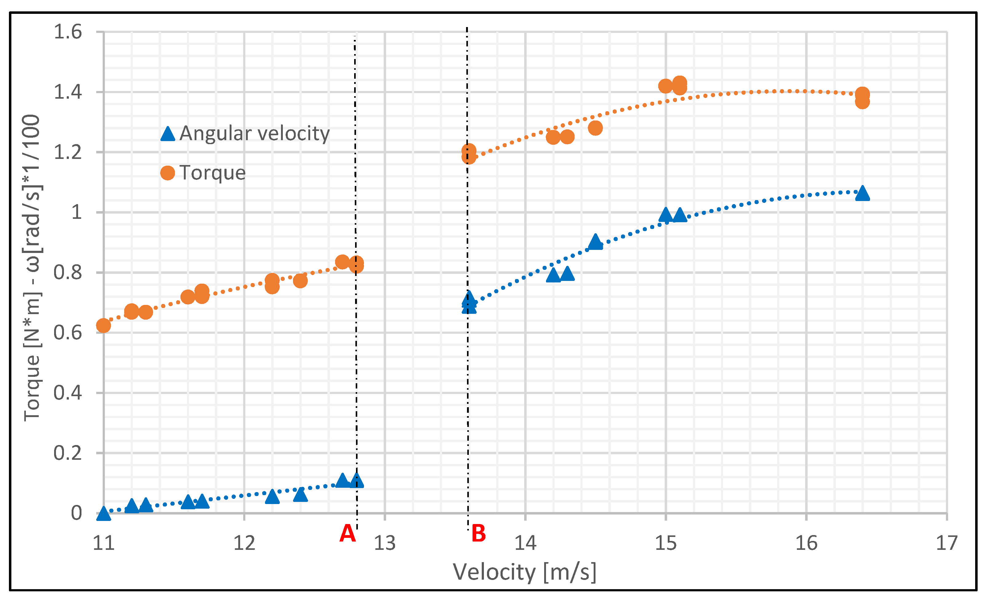
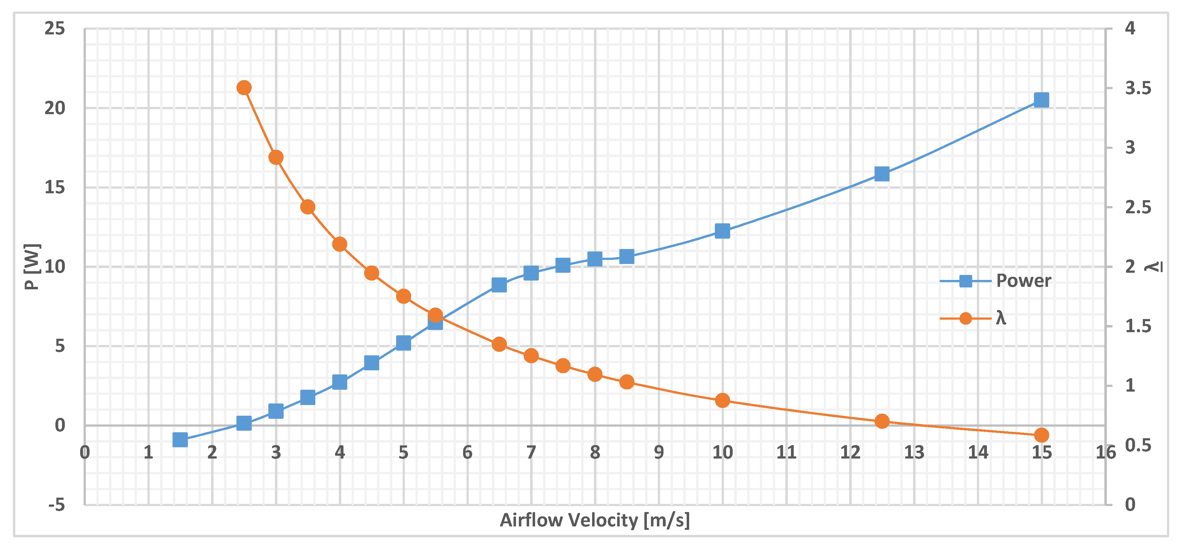
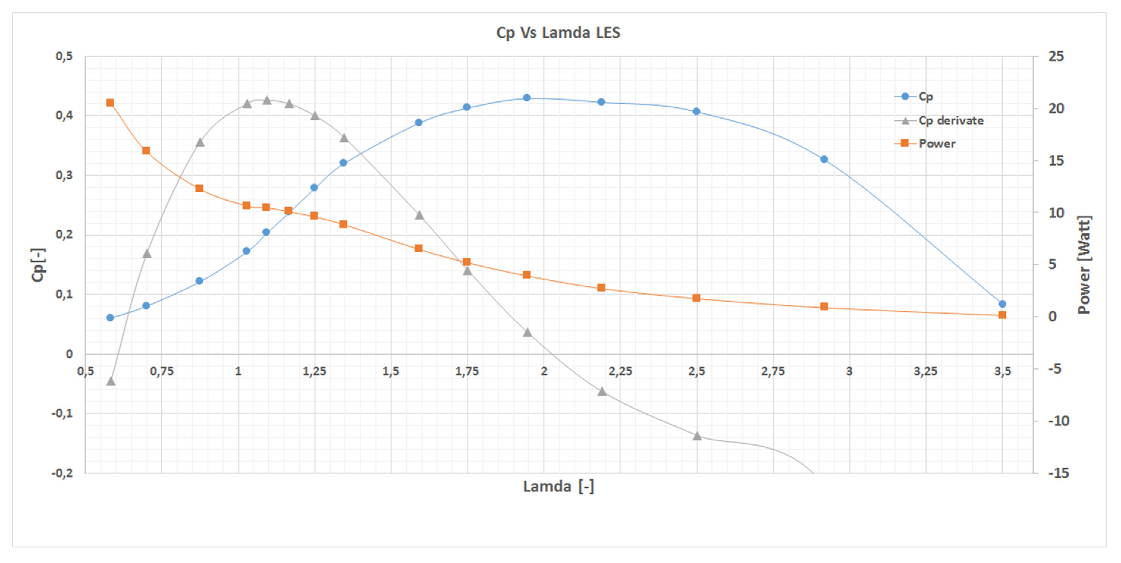
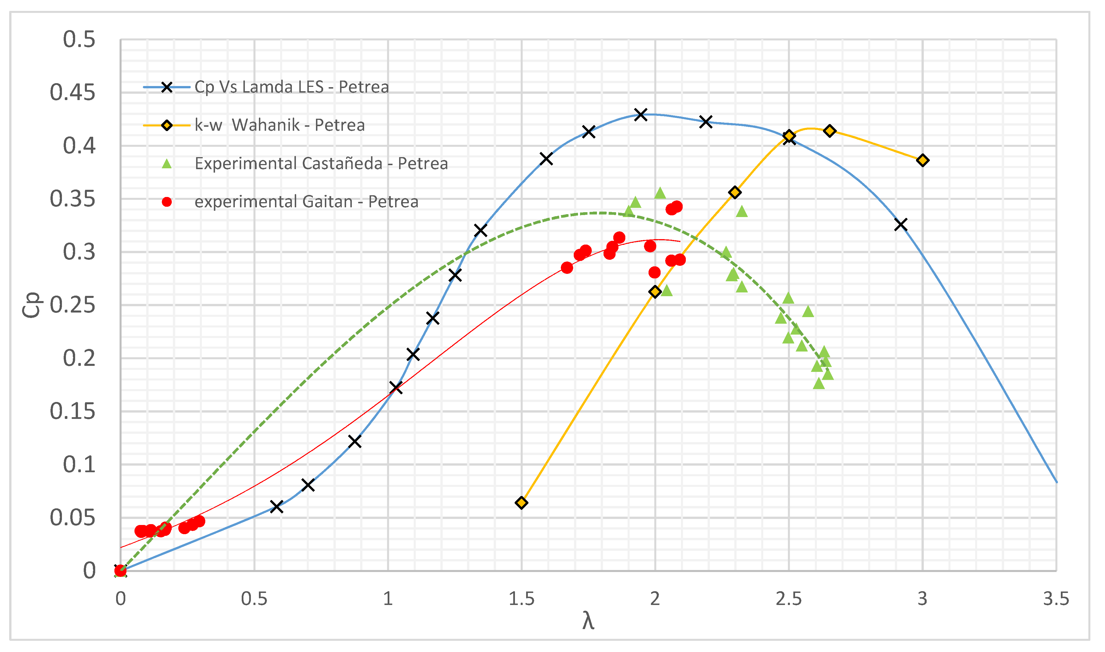
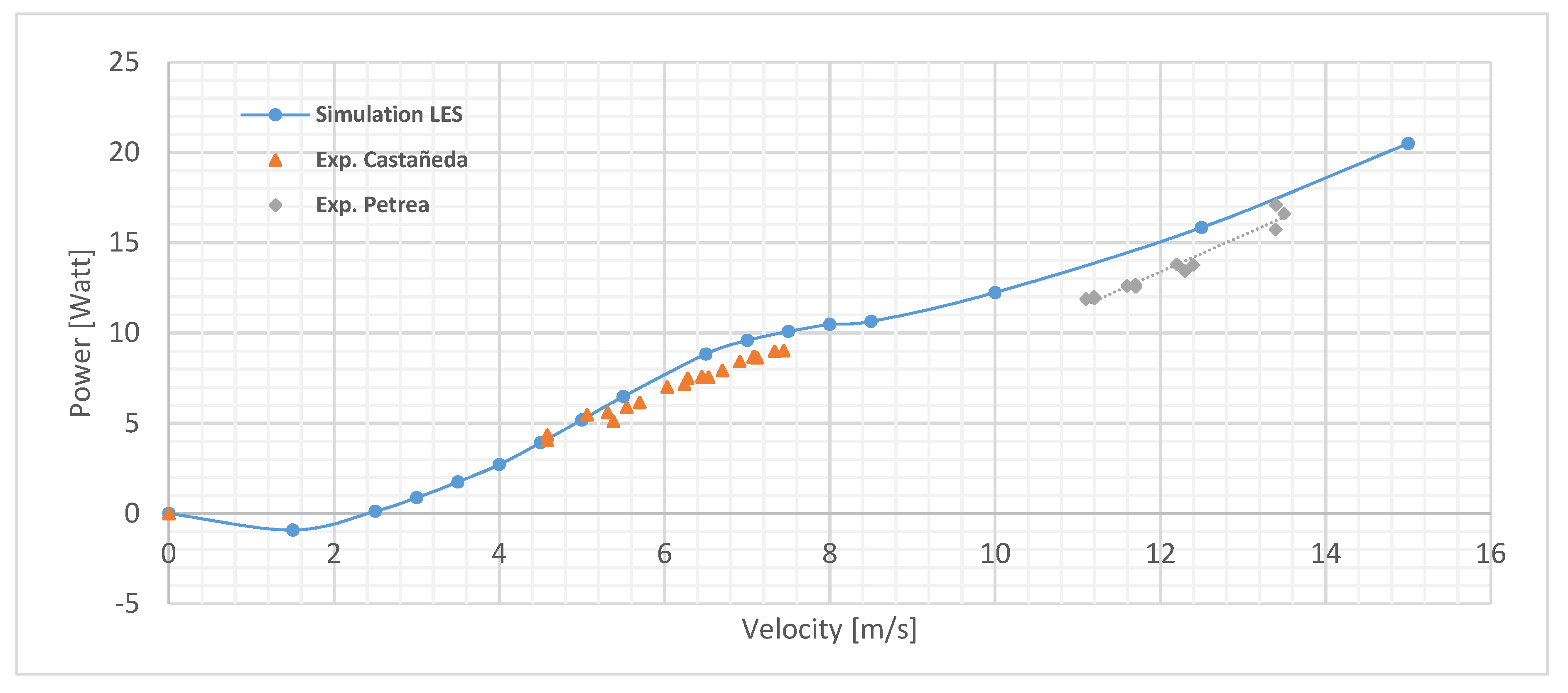
In this work, experimentation and a CDF analysis were developed for Petrea Volubilis (Machigua) rotor. xperimental results show that variable rotor blade pitch angle for maximum performance was obtained in the configuration of 15°: this pitch angle was analyzed with CFD using an LES turbulence model of Large Eddy Equation. It was noted that Machigua rotor predictions from CFD show potential to be useful in low upstream velocities, due to a fast increase in Cp for relatively small increases in upstream velocity from 2.5 m/s, where power is 0 for power predicted up to a maximum in Cp of 0.429 for an upstream velocity of 4.5 m/s. The experimental Cp value is higher than Cp from CFD prediction in 21%, where there is a Cp maximum value of 0.35 in the range of 1.94 < λ < 2.7. The difference between CFD prediction results and experimentation is due to the presence of the measuring device, which generates disturbances in the flow downstream of the rotor, causing differences in Cp values. Similar predictions on the power curve (experimental and CFD prediction) give differences in two different upstream velocity ranges. First, a range from 4.58 to 5.06 m/s, where, comparing CFD with results from Castañeda, power predicted for both velocities are 4.04 and 5.47 Watt, respectively, and experimental results on both velocities are 2.78% and 5.3% lower, respectively, than the CFD power results. The second range from 11.1 to 13.5 m/s gives a difference for both power results of 13.9% and 6.15%, lower than CFD prediction.

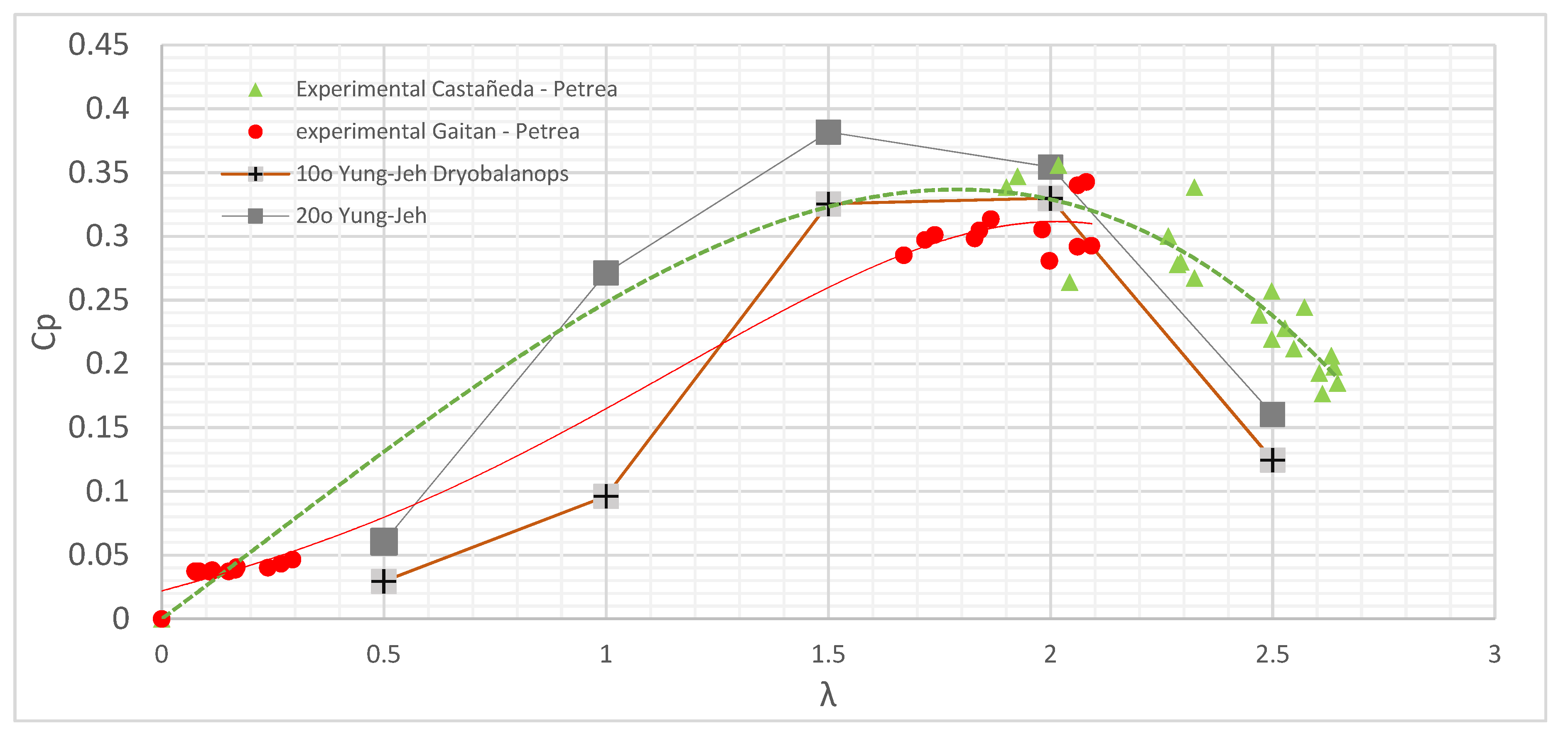
Dryobalanops aromatic rotor [13] modification using three blades rather than five was compared with the Machigua rotor. Dryobalanops rotor Cp curves with a pitch angle of 10° and 20° have similar performance curves to the Machigua wind rotor. A maximum Cp value for Dryobalanops of 0.329 has a 7.42% lower value for Machigua for pitch angle of 10° on λ = 2 for Machigua and λ = 1.5 for Dryobalanops. A difference for Dryobalanops with 20° of pitch angle gives a higher Cp maximum value of 0.38 and a 16.1% lower value for Machigua. This similar response in the Cp curve makes both rotors similar for power generation on lower upstream velocities. This study shows that Machiguá rotor has power transformation potential compared with similar rotors and it is interesting for future investigation to optimize the shape cross-section of the blade in order to keep the maximum lift to drag ratio by using NACA airfoils.