Developing a Mathematical Model for Wind Power Plant Siting and Sizing in Distribution Networks


1
College of Engineering and Science, Victoria University, Melbourne 3011, VIC, Australia
2
Engineering Institute of Technology, Melbourne 3000, VIC, Australia
3
Institute for Sustainable Industries and Liveable Cities, Victoria University, Melbourne 3011, VIC, Australia
*
Author to whom correspondence should be addressed.
Energies 2020, 13(13), 3485; https://doi.org/10.3390/en13133485
Submission received: 22 May 2020
/
Revised: 30 June 2020
/
Accepted: 3 July 2020
/
Published: 6 July 2020
(This article belongs to the Section F: Electrical Engineering)
Abstract
:Wind Power Plants (WPPs) are generally located in remote areas with weak distribution connections. Hence, the value of Short Circuit Capacity (SCC), WPP size and the short circuit impedance angle ratio (X/R) are all very critical in the voltage stability of a distribution system connected WPP. This paper presents a new voltage stability model based on the mathematical relations between voltage, the level of wind power penetration, SCC and X/R at a given Point of Common Coupling (PCC) of a distribution network connected WPP. The proposed model introduces six equations based on the SCC and X/R values seen from a particular PCC point. The equations were developed for two common types of Wind Turbine Generators (WTGs), including: the Induction Generator (IG) and the Double Fed Induction Generator (DFIG). Taking advantage of the proposed equations, design engineers can predict how the steady-state PCC voltage will behave in response to different penetrations of IG- and DFIG-based WPPs. In addition, the proposed equations enable computing the maximum size of the WPP, ensuring grid code requirements at the given PCC without the need to carry out complex and time-consuming computational tasks or modelling of the system, which is a significant advantage over existing WPP sizing approaches.
1. Introduction
Wind power is one of the most abundant, sustainable, cost effective and clean fuel energy sources [1,2]. The majority of small wind farms are being connected to distribution networks [3]. Increasing the penetration of Wind Power Plants (WPPs) in a distribution grid is subject to providing the voltage stability requirements defined by the grid codes. For example, the Australian and UK grid code requires continuous control of steady-state voltage at the Point of Common Coupling (VPCC) of a distribution network connected WPP, with a set point voltage ranging from 95% to 105% of the grid rated voltage [4]. Furthermore, the step-VPCC variation in response to the changes in wind power penetration should generally be maintained at less than 3% [5]. Nevertheless, two main reasons have incurred challenges in meeting the requirements for grid code: the provisions of WPP design regarding the placement of the Point of Common Coupling (PCC), and the limitations in WPP capability to control the terminal voltage [6].
In a distribution grid connected WPP, the overall system impedance angle (X/R) ratio seen at the PCC (X/RPCC) and the Short Circuit Capacity (SCC) are important parameters that affect VPCC stability [7,8]. Short Circuit Ratio (SCR), defined as the grid’s SCC divided by the power generated by WPP (Pwind) [9], is another determining factor. A SCR greater than 20 signifies that the stability requirements of the grid codes have been satisfied [10]. At a given point of a distribution system, SCC is proportional to the square of the system nominal voltage and inverse of the magnitude of system short circuit impedance (Zsc) seen at this point [11]. Generally, the wind velocity is high at sites located far from the distribution substation. Therefore, WPPs are usually connected to the distribution systems through long lines, which makes the Zsc value measured at the PCC large and the values of SCC and SCR small. The SCR value in many grid-connected WPPs is less than 10. The small values of the SCR leads to substantial difficulties to keep the VPCC profile and step-VPCC variations in the limits of steady-state standard defined by the grid codes [12]. Hence, it is critical to determine the optimal size of WPP and select the best site for the interconnection of the WPP to the grid in a way that the grid code requirements, in regards to steady-state voltage stability, are satisfied.
The optimal siting and sizing of Distributed Generators (DGs) in distribution networks has been addressed in literature by the use of analytical methods through improving the voltage stability and minimising the power loss [13,14,15]. The analytical approaches mainly rely on calculating the bus impedance matrix, the inverse of the bus admittance matrix, and the Jacobean matrix. The large size and complicated structure of distribution systems, however, detrimentally affect the efficiency of the algorithms developed for calculating these matrices. Moreover, the assumptions used for the simplifications of calculating Jacobean, impedance and the inverse of bus admittance matrices are not valid in distribution systems [16]. In particular, the inverse of admittance matrix is not applicable to distribution systems consisting of overhead lines as the shunt admittance of the overhead lines is ignorable resulting in singular admittance matrix [17].
A. Onlam et al. proposed an optimization algorithm for power loss reduction in a distribution system through network reconfiguration and DG installation [18]. Their algorithm is based on the simulation model of a 16-bus distribution network. However, the efficiency of the algorithm proposed in [18] is adversely impacted when it is applied into complex networks with a large number of buses.
Artificial intelligence has been widely used in the optimal sizing and interconnection siting of DG units. The efficiency of a method based on the Genetic Algorithm (GA) was compared with that of an analytical method by Pisica et al. [19] in the optimal siting and sizing of DG units in an IEEE 69-bus distribution network. The analytical method was based on nonlinear optimization. The results show that GA can provide a higher accuracy compared with the non-linear optimisation method when the number of DGs connected to the test distribution system is large. On the other hand, the results achieved by both approaches had similar accuracy when the number of DGs is small. Therefore, the results demonstrated that the analytical technique cannot effectively deal with the system complexity as the number of DGs increases, while GA does not require any computational derivatives. However, the main drawback of the GA-based method proposed in [19] is that it requires modelling the entire power system. Other Artificial intelligence-Based approaches for optimal sizing and siting of DG units presented in literature includes Particle Swarm Optimisation (PSO) [20], simulated annealing (SA) [21], the hybrid genetic algorithm (HGA) [21], an Artificial Bee Colony (ABC) [22] and the decision-making algorithm [23]. These approaches require modelling and simulating complicated test distribution systems.
The authors of [24] presented a strategy for the optimal siting of wind farms considering the local wind potential of a given interconnection site, wind speed correlations to other interconnection points and their installed capacities. The main advantage of their work is to simplify WPP site allocation by removing the need to model the system. However, their studies lack the investigation of the impact of WPP interconnection on the voltage stability. Golieva proposed an appropriate approach for the siting of wind farms into distribution networks by developing a numerical relation between VPCC and the system SCR. The proposed relation enables to predict the voltage value at a given distribution feeder and find the optimal size and interconnection site of WPP while ensuring that the voltage regulation requirements are provided without carrying out complex calculations and the computational modelling of test systems. However, the author did not take into account all the steps required for validating the developed relations. For instance, the analysis was performed on a test system having SCR in the range of 0 and 2.5. According to the guidelines provided by Australia Energy Market Operator (AEMO) [25], the wind turbine generator may trip when SCR < 2, indicating that the SCR value should not be less than 2 in actual systems. This demonstrates that the numerical relations developed in [26] cannot be applied in practice. In addition, the main disadvantage of the aforementioned work is that it does not consider the relation between the VPCC and X/RPCC ratio. As discussed earlier, in distribution networks, the VPCC stability has a high dependency on X/RPCC. Therefore, the validation of the equation proposed in [26] is adversely affected due to the lack of consideration of the relation between VPCC and X/RPCC.
Referring to the previous works reviewed in this section, the majority of existing techniques applied for finding optimal size allocation of DG systems require complicated computational tasks and/or designing the simulation model of the entire distribution systems. Furthermore, the limited number of previous works conducted to simplify the WPP siting and sizing did not consider the effect of all critical parameters on the voltage stability at the PCC point. These issues adversely impact the usability of the existing approaches for the sizing and siting of WPPs in distribution networks. Sifting the literature, it was observed that there is a knowledge gaps regarding:
- A simple WPP sizing and allocation approach: As discussed, the existing DG sizing and allocation methods suffer from complex calculations, modelling, and simulation issues. Therefore, a simple approach that does not require the analytical or simulation model of the distribution system is still a noticeable gap in the literature
- A holistic mathematical relation for WPP sizing and siting: The problems of existing DG placement and sizing methods in regard to calculating large and complex dimensional matrices and modelling the entire test system can be removed using a holistic mathematical model between steady-state VPCC and the key parameters of distribution systems. However, only one reference [26], addressed this issue by developing a mathematical relation between VPCC and SCR. The work did not consider the necessary factors needed for validating the results, such as consideration of X/R as one of the parameters of the proposed equation or the realistic range of SCR ratio.
The novelty of the work is to develop a new mathematical approach in response to the existing challenges of analysing the optimal siting and sizing of WPP as mentioned above. This work stems from our previous research [27,28]. The voltage stability analysis carried out in [27] demonstrated that there is a relation between VPCC, SCC and X/RPCC and Pwind. However, in [27], the relation between the aforementioned parameters were presented using power–voltage and reactive-power–voltage curve characteristics and the work has not proposed a mathematical relation between the parameters. The analysis studies carried out in [27] was further developed in our work in [28] by proposing an initial voltage stability mathematical model to show the relation between VPCC and key distribution network connected to Induction Generator (IG)-based WPP. However, the model presented in [28] lacks the investigation of WPPs that are based on the Double Fed Induction Generator (DFIG), which is one of the most common type of WTGs. In addition, the mathematical model developed in [28] has not considered all the steps required for validating the developed relations such as verifying the model using test systems that are different from those used for developing the model.
The hypothesis in this research was to create a holistic mathematical voltage stability model to simplify the sizing and siting of IG- and DFIG-based WPP in distribution network. The proposed model relies on the mathematical relation between PCC bus voltage and the PCC characteristics of a distribution network penetrated by IG- and DFIG-based WPP. The objectives of this research were to:
- Propose a novel voltage stability mathematical model demonstrating the mathematical relations between VPCC, Pwind, SCC, and X/RPCC.
- Validate the accuracy of the proposed analytical model in predicting three important voltage stability criteria at a given connection point of a distribution network penetrated by wind power, including: VPCC profile, step variation of VPCC due to the change of Pwind (ΔVPCC), and the WPP maximum permissible size ensuring the grid code requirements (Pmax), using standard test systems.
To achieve the aforementioned aims, a sensitivity analysis was first carried out to gather datasets, which were used to identify a numerical relation between the voltage and X/R ratio at the PCC of various IEEE test systems with different SCR values. Analysis was carried out based on both IG and DFIG. For each generator type, the obtained V-X/R data points were then used to develop general forms of equations capable of modelling the relations between the voltage, Pwind, and the PCC parameters. A Genetic Algorithm (GA)-based approach was then used to identify the coefficients of the developed equations. The accuracy of the proposed equations was then evaluated using different scenarios involving a wide range of operating conditions. The methodology proposed is based on all critical parameters that impact the voltage stability at potential distribution system WPP interconnection point. Therefore, the model enables to predict the important voltage stability criteria at a given PCC site. Using the predicted criteria, the design engineers can select the optimal site and size of WPPs in distribution grids, ensuring that the grid code requirements in regard to the voltage stability are provided.
Achieving the aforementioned aims made this work a leader in the research deals with modelling the mathematical relations between the key parameters of distribution network connected WPPs and main voltage stability criteria at the PCC. The mathematical relations enable prompt computation of the size of a WPP. It also enables the identification of the appropriate PCC buses in which it is assured that VPCC profile and ΔVPCC are in the standard range defined by the grid codes given the SCC and X/RPCC values. In the proposed mathematical model, the key PCC parameters, i.e., SCC, X/RPCC, are the only unknown of the developed equations. These parameters are usually available as the baseline characteristics of the distribution grid connected WPPs or can be easily calculated at any point looking back to the distribution substation. Hence, the proposed equations enable WPP siting and sizing without the need to solve complex and time-consuming computational tasks, which is the main advantage of the presented method over the existing approaches.
The paper is organized as follows: Section 2 presents the methodology and the specific steps carried out in this study to propose the mathematical model, including: the modelling test systems used for providing data needed for developing a series of alternative equations, identifying the coefficient of the developed equations using a GA-based approach, determining the most accurate equations among the developed alternative equations and proposing the final form of the mathematical model. Section 3 demonstrate the significance of the methodology proposed by comparison with the main previous works available in literature. The accuracy of the proposed model in predicting the critical voltage stability criteria was investigated in Section 4, and, then, Section 5 summarizes the major conclusions of this study.
2. Developing Mathematical Formulations
As discussed in Section 1, this paper aims to develop the mathematical relationships between VPCC, WPP size and inherent PCC characteristics of a distribution system, including: the SCC and X/RPCC ratio through voltage stability analysis studies. This was primarily conducted by investigating how VPCC behaves in response to changes in X/RPCC for networks with different SCC and SCR ratios. Analysis was preformed based on two types of generators most commonly used in wind turbines: the Induction Generator (IG) and the Double Fed Induction Generator (DFIG). Different steps followed for developing the proposed mathematical model have been presented in the sub-sequent sections.
2.1. Methodology
The overall methodology used in developing the mathematical formulations is presented below.
Modelling the test systems and measuring the SCR ratio for each system: Four distribution system models defined by the Institute of Electrical and Electronics Engineers (IEEE) were simulated and considered to provide data required for developing the mathematical relations. After modelling the test systems using MATLAB/Simulink (version 2019 developed by MathWorks, Natick, MA, USA) the short circuit current value was obtained at the PCC of each system. The Isc values were obtained and then the grid’s SCC was calculated using (1). Finally, the SCR value was given by (2) regarding the amount of power injected by the wind farm in each test system.
where Vrated is the nominal voltage of the distribution feeder, Isc is the short circuit current at the PCC and Pwind is the amount of power generated by WPP.
Plotting VPCC-X/RPCC characteristics: For each test feeder modeled in the previous step, the X/RPCC ratio was measured and varied under a fixed SCC and SCR network. The X/RPCC ratio was changed throughout the course of the analysis by changing the X/R ratios of the distribution lines. Then, VPCC value was recorded taking note of the variations in response to the change of the overall X/RPCC ratio. The VPCC versus X/RPCC characteristic has been plotted for each test feeder using the obtained data.
Developing alternative mathematical functions modelling the relations between VPCC, X/RPCC, SCC and Pwind: The voltage behaviour, with respect to changes in the X/RPCC ratio, was then analysed for all test systems to mathematically correlate VPCC, X/RPCC, Pwind and SCC. At the end of this step, the general forms of alternative equations, which can be used to describe the relation between the aforementioned parameters were developed. Then, the coefficients of the equations were identified using an Artificial Intelligence (AI)-based approach.
Determining the best fit function: The accuracy of each alternative equation was investigated in order to identify the best fit equations.
Developing the final form of the functions: Finally, it was investigated how the functions presented in the previous step can be further developed for different operating conditions.
Details about the aforementioned steps are provided in Section 2.2, Section 2.3, Section 2.4, Section 2.5 and Section 2.6.
2.2. Modelling Test Systems
In this paper, four test distribution networks were modelled and simulated to develop the mathematical formulations. The adoption of four systems was to take into account various values of SCC and X/RPCC and hence develop a formulation with higher validity. The modelling of two test systems, referred to as Test 1 and Test 2, relied on the 37-bus IEEE distribution network (Figure 1), while the modelling of other two test systems, referred to as Test 3 and Test 4, was based on the 9-bus IEEE distribution network (Figure 2). The PCC was considered to be at Bus 9 in the 9-bus system and at Bus 6 in the 37-bus system. The size of the WPP and the length of the lines are different amongst the four test systems, resulting in different values of SCC and SCR.
In each model, the distribution system is connected to a 120 kV, 50 Hz external source of infinite short circuit current through a Yg/Δ configuration of a three-phase distribution transformer. Furthermore, in each model, a WPP with the total rated capacity of 9 MVA, provided by three 3 MVA WTGs, is connected to the distribution system at the PCC. A three-phase transformer with Yg/Yn configuration is connected to each WTG to boost the generator terminal voltage to the rated voltage of distribution system, i.e., 22 kV. The parameter values of different components of the simulated models are presented in Table A1, Table A2, Table A3 and Table A4 in Appendix A.
The feeder steady-state voltage before the WPP connections, called Vinitial, has a significant impact on the VPCC stability after the WPP connection. Developing the mathematical relations for a constant Vinitial value hinders the application of the relations for any distribution network, as loading conditions and various voltage regulator set-point values impact the Vinitial value. In this study, it was firstly assumed that Vinitial is around 0.98 pu for each test distribution feeder. Therefore, the mathematical relations were firstly developed regarding Vinitial = 0.98 pu. Then, in Section 2.6, the proposed relations were further developed such that it satisfies a wide range of Vinitial values. The adoption of various Vinitial values in the proposed methodology was to reduce the uncertainty due to the load deviations from the values used in the test systems.
Table 1 presents the values of PCC parameters, including: Isc, SCC, Pwind, and SCR, for each test system.
Among the cases presented in Table 1, Test 1 with the least SCR value, is the weakest system. Moreover, the lowest value of SCC and Pwind is seen for Test 4 with the greatest SCR value, which is due to the small Pwind. This results in the PCC point in Test 4 being the stiffest among other test systems.
2.3. Characteristics of Voltage-X/R Ratio at the PCC
In this paper, the proposed methodology is based on the VPCC-X/RPCC data obtained from simulation models. The reason for using simulation models for obtaining VPCC-X/RPCC data is the fact that the development of mathematical relations with an appropriate accuracy requires a large number of data points. The lack of such a data base adversely impacts the accuracy of the mathematical relations. The use of simulation models enables to provide a large number of data by carrying out sensitive analysis through changing the X/RPCC ratios and monitoring VPCC taking note of the variations against the change of the X/RPCC ratio. The X/RPCC is an inherent characteristic of a power system and cannot be dynamically changed in an actual network. Therefore, having access to a large quantity of VPCC-X/RPCC data points obtained from actual systems is a complicated process.
From a practical perspective, the application of the proposed analytical model to the real-world distribution systems may impose additional complexity and challenges due to the uncertainty of the simulation models. To enhance the accuracy of the proposed model against the issues concerned with the uncertainty of the simulated test systems, the range of the X/RPCC ratio, analysed in this study, was derived from an analysis of actual distribution networks performed in [29]. Reginato et. all [29] carried out a research study concerned with an analysis of the effect of X/RPCC and the inverse of SCR, the so-called integration level (p), on VPCC using data from actual systems. The analysis was performed to determine a potentially viable X/RPCC range, ensuring the grid code requirements with regard to the steady-state VPCC stability for a given integration level. The analysis results were presented using p vs X/RPCC graphs, while 0.95 pu < VPCC < 1.05 pu. Although the authors in [29] did not present the value of VPCC for a given X/RPCC and p, the realistic range of X/RPCC has been identified for different integration levels using data obtained by actual systems. In the VPCC-X/RPCC characteristics presented in this section, the range of X/RPCC and the corresponding SCR value are based on the p-X/R graphs presented in [29] to decrease the issues related to the uncertainty of the data obtained from simulation models, i.e., VPCC- X/RPCC data points, in case of real application.
To draw the VPCC/X/RPCC curve characteristics, the X/RPCC ratio of the test systems in Section 2.2 was changed to observe the VPCC values for each X/RPCC with SCC and SCR values of the test system being constant. The data points collected were utilised to plot the characteristic of VPCC against the X/RPCC ratio. The results are presented in Figure 3.
For the IG-based WPP, Figure 3, in X/RPCC around 2, the VPCC values for all four systems are nearly equal. This observation is in accordance with [29], which states that the lowest variation in voltage happens at X/RPCC = 2 irrespective of the SCR value in an IG-based WPP, which is another piece of evidence to confirm that the methodology results are based on realistic cases.
The PCC voltage for both IG- and DFIG-based WPPs is high at the points with a low ratio of X/RPCC (X/RPCC < 2). This is particularly apparent in small SCR ratios. For example, from Figure 3, it can be seen that the PCC voltage of Test 1 with an SCR ratio equal to 3 is greater than the maximum acceptable voltage level defined by the grid codes (VPCC > 1.05 pu) when the X/RPCC ratio is smaller than 0.5. This is in contrast with Test 4 with the maximum SCR ratio equal to 7, where the low values of the X/RPCC ratio do not cause a noticeable increase in the voltage. When dealing with large X/RPCC ratios, Figure 3 demonstrates that the voltage variation due to changes in wind power penetration is negligible at the connection point of a DFIG-based WPP with X/RPCC > 2. Furthermore, Figure 3 shows that voltage at the PCC of IG-based WPP is small when the X/RPCC ratio is large (X/PPCC > 2). The variations in voltage according to a rise in X/RPCC ratio is more remarkable at the weaker test feeders. In Figure 3, Test 1 shows a VPCC value less than the minimum limit of the allowable range, i.e., VPCC < 0.95 pu, when X/RPCC is around 2.5. The voltage for Test 4 is shown to be within the standard range, even in X/RPCC ratios greater than 5.
2.4. Developing Alternative Functions
In this section, the main aim is to present the mathematical relations which can model the VPCC-X/RPCC characteristics shown in the previous section. The relations were developed for the values of X/RPCC that imposes Power Quality (PQ) concerns and voltage regulation problems at the PCC. Therefore, both small and large X/RPCC ratio ranges were considered for developing the formulation for the IG-based WPP. Furthermore, only small X/RPCC ratios were considered for expressing the mathematical relations for the DFIG-based WPP.
2.4.1. General Form of Alternative Functions for IG-Based WPPs
Mathematical formulas were developed to introduce the best fit curve for the VPCC-X/RPCC data points presented in Figure 3. Two key features in Figure 3 were considered in developing the equations, which are presented in Table 2.
Two possible functions, including an exponential function and a polynomial function with an order of 2, were proposed and investigated to cover the characteristics listed in Table 2. The general forms of the functions are as follows:
- Function 1—Exponential function
- Function 2—Polynomial with an order of 2where Z0, Z1, Y0, Y1 and Y2, are positive coefficients. γ and δ represent the exponential and polynomial decay coefficients, respectively.
Mathematically, it can be tested and confirmed that the VPCC-X/RPCC characteristic curves given by (3) and (4) have similar patterns for all X/RPCC ranges and different decay coefficients. Hence, both functions can be applied to model the relation between VPCC and X/RPCC. Figure 4 shows the general VPCC-X/RPCC curve of the considered alternative functions for different values of decay coefficients.
Figure 4 for (3) and (4) shows that smaller decay coefficients (γ and δ) increase the PCC voltage. Looking at the first characteristic presented in Table 2, small SCR values increase voltage at the PCC points with a small X/RPCC ratio. Therefore, it can be concluded that SCR and the decay coefficients are directly related when X/RPCC is small (X/RPCC < 2), expressed by (5) and (6).
where K1 and K2 are considered positive.
Figure 4 demonstrates that higher values of decay coefficients results in a decrease in VPCC. Referring to the second characteristic explained in Table 1, small SCR values decrease voltage at the feeder with a large X/RPCC ratio. Hence, SCR and decay coefficients have an inverse relationship when X/RPCC is large (X/RPCC > 2). This relationship is given by (7) and (8):
where K3 and K4 are considered positive.
Noting the relation between decay coefficients and SCR given in (5) to (8), the alternative functions (3) and (4) can be rewritten as (9) to (12).
where Zs0, Zs1, Ys0, Ys1 and Ys2 are positive coefficients in the equations representing the small X/RPCC range (X/RPCC < 2) and Zl0, Zl1, Yl0, Yl1 and Yl2 are positive coefficients in the equations representing the large X/RPCC range (X/RPCC > 2).
2.4.2. General Form of Alternative Functions for DFIG-Based WPPs
Comparing the results obtained for IG- and DFIG-based WPPs shown in Figure 3, the VPCC variation against changes in X/RPCC follows a similar pattern in both IG- and DFIG-based WPPs when X/RPCC < 2. Hence, the VPCC-X/RPCC curves plotted for DFIG and IG are similar to each other in the small X/RPCC ratio, where DFIG cannot efficiently regulate the voltage. This signifies that the alternative functions applied for the DFIG-based WPP are similar to those developed for the IG-based WPP with small X/RPCC. The general forms of the functions are expressed in (13) and (14).
where Ws0, Ws1, Ws0, Us0, Us1, Us2 and K5 are positive coefficients.
Due to the crucial effect of the coefficients on the accuracy of Equations (9)–(14), the next section is devoted to determining these coefficients by the use of a GA-based approach.
2.4.3. Determining the Coefficients Values Using GA
The Genetic Algorithm uses an exploratory approach to optimise a given objective function utilising the ideas of evolutionary processes [30]. Although GA is available in the MATLAB Optimization Toolbox, coding is required for defining the objective function and GA parameters.
The value/type of the most important GA parameters considered in developing the mathematical model presented in this paper is tabulated in Table 3.
The default number of generations and population size in the MATLAB GA toolbox are 100 and 20, respectively. As shown in Table 3, the generation and population sizes considered in this paper are noticeably larger than the default values increasing the accuracy of the GA outputs. From Table 3, the selection of individuals in current generation as the parents for the next generation is based on stochastic uniform, which provides the highest accuracy compared with other search strategies defined in GA [31]. Furthermore, the type of crossover parameter, which classifies two parents of the intermediate generation to build a new individual for the next generation, is ‘scattered’ as it provides higher flexibility compared with the other types of the crossover functions [32]. It can also be seen from Table 3 that the type of mutation function is constrained dependent. Another important GA parameter is mutation, which makes small randomly changes in the genes of parents to create mutation individuals for the next generation [33]. Mutation function is categorised into two types: unconstrained and constrained dependent. As shown in Table 3, in this study, a constrained dependent mutation function has been used and the constraints are related to the upper and lower boundaries of the input parameters of the objective functions.
A separate objective function has been coded for each Equation in (9)–(14), which resulted in 6 objective functions, as shown in Table 4.
From Table 4, the values of the input parameters of Objective Functions 1 to 6 (Func1 to Func6) represent the values of the coefficients of (9) to (14), respectively. In each objective function, the coefficient of the corresponding equation was considered as the input parameters, while the error between predicted graph and the reference VPCC-X/RPCC curve was considered as the output parameter. The main idea was to find the coefficient of each alternative equation in a way that the curve predicted and plotted by the equation has the lowest error with respect to the corresponding reference VPCC-X/RPCC curves shown in Figure 3. The error was calculated using Standard Deviation (SD) formulas.
For clarifying the operation of the objective functions, Figure 5 presents the flowchart diagram for one of the objective functions used for finding the coefficients of (9), named Func1.
Once the objective function has been coded and GA parameters have been defined, the optimal values of the function input parameters was determined by running a separate GA for each objective function. GA was responsible to find values of the input variables for which the output of the objective function becomes minimum. The values are as shown in Table 5, Table 6 and Table 7.
Utilizing the coefficient values from Table 5, Table 6 and Table 7, Equations (9)–(14) were rewritten to give Equations (15)–(20).
- IG-based WPP with X/RPCC < 2:
- IG-based WPP with X/RPCC > 2:
- DFIG-based WPP with X/RPCC < 2:
2.5. Finding the Fit Functions
The best fit function with the least amounts of errors compared with the reference VPCC-X/RPCC data points was obtained for Equations (15)–(20). As stated in Section 2.4.3, the output parameter for GA objective functions was considered to be the error between reference and predicted values and was calculated by SD formulas. In addition to SD, the Mean of Relative Error (MRE) and the Mean of Absolute Error (MAE), as two frequently used criteria, were considered for evaluation of the error in this section.
For each alternative function and test system, the error between the reference and predicted VPCC-X/RPCC curve characteristics were calculated using SD, MRE and MAE formulas, as shown in (21) to (23).
where the reference values of VPCC is expressed as Vk, and its predicted values are expressed as . Moreover, the total number of reference values is given as m.
The values of the three factors used for evaluating the error between the reference and predicted VPCC-X/RPCC values have been presented in Table 8 for each alternative function and test system. Furthermore, the difference between the reference VPCC-X/RPCC curve characteristics obtained by the simulation results and the VPCC-X/RPCC curve characteristics plotted by the developed alternative equations can be compared for each test system using graphical representation, as shown in Figure 6a–l.
Based on Table 8, in IG-based WPP with X/RPCC < 2 for all test cases, the evaluation criteria calculated for (15) is less than the criteria obtained for (16). This is confirmed in Figure 6a–d, where the curve for (15) shows a smaller error than the curve for (16) compared with the reference curve. Analysis of IG-based WPP with X/RPCC > 2 for all test cases based on Figure 6e–h and Table 8 reveals a slightly higher accuracy for (18) compared to (17).
In the case of DFIG-based WPP, Figure 6i–l and Table 8 show that the exponential function provides less error compared to the polynomial function. Therefore, according to the statistical and graphical results presented, the best fit functions are as listed in Table 9.
The mathematical relations developed in Section 2.2 is based on an initial voltage of 0.98 pu for the test systems, hence Equations (15), (18) and (19) would be only used for the feeders with Vinitial of 0.98 pu. Nevertheless, the initial voltage varies from the default value because of the loading conditions and values of voltage regulator set-point. Consequently, another set of equations is required to calculate the voltage stability criteria at a certain test system with any initial voltage value.
2.6. Developing the Final Form of the Functions
To establish the final form of the developed mathematical equations, the best fit functions presented in Table 9 were further developed for various initial voltage levels. The impact of variations in the initial voltage on the Pwind versus VPCC curve was evaluated using simulation systems characterized in Table 1. The initial voltage was varied in the simulations from the default value (Vinital = 0.98 pu) to plot the variations of Pwind against VPCC for each new voltage value. The shape of the curves remained the same with both the default and varied initial voltages. The only difference was a downward shift for initial voltages less than 0.98 pu and an upward shift for the initial voltages greater than 0.98 pu. Defining ΔVinitial = Vinitial - 0.98, it can be approximated that for a given initial voltage, the addition of ΔVinitial to the PCC voltage value calculated by the equations in Table 9 gives the voltage value at PCC point. Hence, Vinitial parameter was incorporated in (15), (18) and (19) to give (24)–(26) in Table 10, respectively.
As the SCR is equal to the ratio of the grid’s SCC to Pwind, Equations (21)–(23) can be rewritten to calculate optimal value of wind power generation (Pmax) such that the voltage value at PCC point is kept in the standard range. To do so, in Equation (25) related to WPP with large X/RPCC, the voltage value at the PCC point was assumed to be 0.95 pu, which is the minimum allowable voltage level defined by the Australian grid code. In Equations (24) and (26), developed for WPP with a small X/RPCC ratio, the voltage at PCC point was assumed to be equal to the maximum limit of the admissible steady-state voltage.
After determining the VPCC values, the equations were rewritten in terms of Pwind as a function of PCC parameters and Vinitial as can be found in (27) to (29) in Table 10.
3. The Significance of Proposed Model
In this section, the proposed mathematical model is compared with the main previous works available in literature to demonstrate the significance of the research performed in this paper and its contribution to the existing knowledge.
The majority of the previous works dealt with the effect of SCC, SCR and X/R ratios on VPCC in general terms and using graphical representation and different curve characteristics such as VPCC versus X/RPCC, VPCC versus SCR etc. For example, Kothari and et al. investigated the general relation between VPCC, X/RPCC and SCR in distribution systems connected WPP [34]. Their work presented the analysis results using the curve characteristic of VPCC versus SCR plotted for different X/RPCC ratios. For the X/RPCC = 0.5 case, the results in [34] demonstrated that the difference between the initial value of VPCC (Vinitial) when Pwind = 0 and the VPCC value obtained for high wind power penetration is around 7%. Referring to (2), the high penetration of wind power makes the SCR value small. Hence, in [34], it was demonstrated that the difference between Vinitial and VPCC after WPP connection is around 7% (ΔVPCC = 7%) when X/RPCC is 0.5 and SCR is noticeably small.
The results presented in [34] were compared with the results obtained by the equations proposed in this paper. For this purpose, the difference between the Vinitial and VPCC values after WPP connection was calculated using proposed equations considering that X/RPCC = 0.5 and SCR is small. The calculations were performed assuming that SCR is slightly greater than 2, i.e., SCR = 2.5. This is because, as mentioned in Section 1, AEMO documentation indicates that an SCR < 2 should be avoided in WPPs, as it adversely impacts the voltage stability in the steady-state operation and may lead to generator tripping [25]. The comparison results have been shown in Table 11.
As shown in Table 11, the results gained by the proposed equations confirm the discussion presented in [34] that the difference between Vinitial and VPCC under high wind power penetration is around 7% when X/RPCC = 0.5. Although the authors in [34] investigated the general relation between VPCC, SCR and X/RPCC using graphical representation, they did not propose any mathematical relation between these parameters. This shortcoming hinders to investigate the voltage variation for any given X/RPCC and SCR values.
In [12,35], it was demonstrated that the steady-state VPCC tends to increase for small X/RPCC ratios, while it decreases for large X/RPCC ratios in weak distribution networks penetrated by DGs. Furthermore, the authors in [36] showed that the voltage drop, due to an increase in X/RPCC, is more serious in distribution systems with low SCR values (weak systems) compared with that in the distribution feeders with larger SCR values (stiff systems). The results presented in [12,35,36] confirm the general characteristics of the functions given by the equations presented in Table 10. However, the authors in these works, only discussed the relation between VPCC, X/RPCC and SCR in a general manner and using graphical representation and their works do not propose a mathematical relation between these parameters.
The author of [26] offer one of the most valuable preliminary works, discussing the mathematical formulation of any formula to express the relationships between VPCC and SCR for the steady-state operation of the WPPs. It was demonstrated that the relation between VPCC and SCR can be expressed through a polynomial function with an order two as shown in (30) [26].
As claimed by the author in [26], taking advantage of this relation, the voltage profile can easily be predicted using the SCR value at each distribution feeder. This is a great achievement as it would allow WPP planning engineers to select the best site for the interconnection of a WPP without the need to carry out complex and time-consuming computational tasks and modelling test systems. However, the accuracy of the equation proposed in [26] is adversely impacted due to the lack of considering the relation between X/RPCC, which is one of the most important characteristics of distribution networks, and VPCC. In addition, the equation was developed using data provided by an invented test system with unrealistic SCR range (0 < SCR < 2.5), which adversely impact the accuracy of (30) in real distribution systems.
Sifting the literature, it is clear that a holistic relation between VPCC and the key parameters of the distribution systems, i.e., the SCR and X/RPCC ratio, is still a noticeable gap. This shortcoming has been eliminated in this paper using the proposed mathematical model presented in Table 10. Furthermore, the proposed equations have been developed using data obtained by IEEE standard distribution networks.
Referring to Table 10, the proposed model enables design engineers to plot the curve characteristic of Pwind versus voltage at a potential distribution network WPP interconnection point using (24) and (26), considering the WTG type and the values of SCC, Vinitial and X/R at that point. Taking the advantage of the Pwind versus voltage curve characteristic achieved by the proposed equations, the engineers can predict the VPCC value for different wind power penetration at a potential interconnection point. The predicted VPCC values enable the grid codes’ compliance check, i.e., to verify if VPCC is between 0.95 and 1.05 pu (compliance with the grid codes) or if VPCC is not maintained within 0.95 and 1.05 pu (grid codes violation), at the interconnection of WPP to a potential interconnection site. The potential site can then be selected for connecting WPP if the grid code requirements are met or identified as an inappropriate PCC point if the grid code requirements are not provided.
As another advantage of the proposed mathematical model, the engineers can estimate the step-VPCC variations in response to changes in wind power penetration at a given PCC point using (24) to (26) depending on the WTG type and the X/RPCC ratio. The predicted results obtained for the step-VPCC variations enables the engineers to decide how many WTGs can be simultaneously switched on, ensuring that the step-VPCC variation satisfies the grid code requirements (ΔVPCC ≤ 3%).
Furthermore, the proposed model enables the network and grid interconnection engineers to find optimal WPP size and estimate the maximum power injection by a WPP to ensure voltage stays within acceptable steady-state limits at a given PCC point using (27) to (29). Therefore, the proposed mathematical model provides design engineers with a series of informative equations to find the optimal size and site of WPP in a distribution network by predicting three critical voltage stability criteria, i.e., VPCC profile, step-VPCC variation and maximum permissible wind power generation, ensuring the grid code requirements.
As discussed in Section 1, the majority of existing approaches used for WPP siting and sizing are based on the modelling and simulation of the whole system and/or calculating the bus impedance, inverse of the bus admittance, and the Jacobean matrices. However, the simulation of distribution networks is a demanding process due to the size and complexity of these networks. Moreover, the assumptions used for the simplifications of calculating Jacobean, impedance and inverse of admittance matrices are not valid in distribution systems. These issues are removed using the proposed mathematical model presented in Table 10. The proposed equations require only three input parameters (Vinitial, X/RPCC and SCC) which are usually available as the baseline characteristics of the distribution systems or can easily be calculated at any point looking back to the distribution substation. Hence, the proposed equations enable WPP siting and sizing by promptly conducting three important voltage stability criteria at a potential distribution network interconnection point. Consequently, it removes the need to solve complex and time-consuming computational tasks or modelling the entire test distribution system, which is the main advantage of the presented over the existing WPP sizing and siting approaches. The proposed analytical model removes the need to investigate the effect of distribution network configuration and its component specifications on PCC bus voltage stability. This is due to the fact that the effect of these factors has been considered and modelled in the proposed analytical approach using SCC and X/RPCC parameters.
The validation of the proposed mathematical model in predicting the aforementioned three voltage stability criteria at a potential distribution network WPP interconnection point has been conducted in the subsequent sections of this paper.
4. Validation Results
This section presents the analyses performed to validate the proposed functions, listed in Table 10, which can be used to project three important VPCC stability criteria, including: VPCC, ΔVPCC, and Pmax for a potential connection site in a distribution network, given the Vinitial value. In this respect, the accuracy of the proposed functions was investigated using two case studies. Case study 1 provides initial validation studies by assessing the accuracy of the proposed mathematical model using the four test systems presented in Section 2 with different X/R ratios and Vinitial values. Then, in Case study 2, the functions developed were applied for a new test system based on a 30-bus IEEE distribution network.
4.1. Case Study 1—Validation for Different Vinitial Values
As discussed in Section 2.6, loading conditions and various voltage regulator set-point values may result in different Vinitial values. Therefore, the effect of load variations and any other factors that change operating voltage at a given distribution feeder before the WPP connection has been modelled using Vinitial parameter. Vinitial has a profound effect on the Pwind versus VPCC characteristic and on the steady-state voltage stability after the connection of WPP. In this regard, the proposed mathematical model should ideally work for any Vinitial value to ensure that the equations developed can be applied for a wide range of distribution networks with different loading conditions. Hence, as an initial assessment of the accuracy of the proposed mathematical model, the equations presented in Table 10 are verified for different Vinitial values. The validation study has been performed using the four test systems applied for developing the mathematical model with details presented in Section 2.2. However, the validation studies were performed considering that the loading conditions and Vinitial values of the four test systems are different from the default value (Vinitial_default = 0.98 pu) considered in Section 2.2.
Two test systems were simulated based on a 37-bus IEEE distribution network and two test systems were simulated based on a 9-bus IEEE distribution network using MATLAB/Simulink as shown in Figure 1 and Figure 2, respectively. For the 37-bus model, the potential distribution network WPP interconnection point was considered to be at Bus 6. Furthermore, the potential site for connecting WPP was considered to be at Bus 9 for the 9-bus model. The topology and/or length of distribution lines are different among the test systems considered making their SCC values to be different. The SCC value and topology of each test system are as listed in Table 1 in Section 2.2.
It is noted that the analysis performed in Case study 1 is the initial stage of validating the proposed mathematical model. In this stage, the SCC values and topology of the test systems used for validation studies are similar to the SCC values and topology of the test systems used for developing the mathematical model. However, the Vinitial values are different from that considered for developing the proposed equations. Therefore, the mathematical model is validated using new operating conditions. In addition, the proposed model is validated for various X/RPCC ratios.
In this section, six scenarios were analysed: two scenarios for the IG-based WPP with X/RPCC < 2, two scenarios for the IG-based WPP with X/RPCC > 2 and two scenarios for the DFIG-based WPP. Table 12 shows the test system, X/RPCC ratio and Vinitial value considered in each scenario. Furthermore, the SCC value and topology of each test system have been re-written in Table 12.
For each scenario, the Pwind versus VPCC curve characteristic obtained by the simulation results is compared with the Pwind versus VPCC curve characteristic given by the corresponding proposed equation presented in Table 10. The results are as shown in Figure 7a–f.
The curve characteristics presented in Figure 7a–f are used to validate the proposed equations in predicting VPCC profile and ΔVPCC.
When predicting VPCC value, the largest error between the reference and predicted results occurs in Scenarios 1 and 5 when wind power is not connected (Pwind = 0). Referring to Table 12, both the SCC and X/RPCC ratio are small in Test 1 and 5. Therefore, the accuracy of the proposed mathematical model is slightly impacted when both the SCC and X/RPCC ratio are small. However, as shown in Figure 7a,e, the highest error is 1%. In the other scenarios considered, the error between the simulation and predicted results is less than 0.5%.
In the case of the prediction of ΔVPCC, the simulation results in Figure 7a–f demonstrate that the proposed equations accurately verify the compliance or violation of ΔVPCC with respect to the grid code requirements. As defined by the grid codes, the ΔVPCC value must not exceed 3%. Comparing the curve characteristics shown in Figure 7a–f, it can be observed that both simulated and predicted results demonstrate that the highest ΔVPCC occurred in Scenario A, where the SCC and X/RPCC are both small. According to Figure 7a, both simulation and predicted results show that the VPCC variation in response to an increase in Pwind from 0 to 3 MVA is greater than 3%. Therefore, the results confirm that ΔVPCC violates the grid code requirement when only one 3 MVA generator is connected to the grid. However, for the same increase in Pwind, ΔVPCC does not exceed the standard range in other scenarios. In the case of scenarios with large X/RPCC (Scenarios 3 and 4), both simulation and predicted results presented in Figure 7c,d demonstrate that ΔVPCC is more serious in Scenario 3, where the SCC value of the test system considered is smaller.
Generally, comparing the simulation and predicted results in Figure 7a–f, it is clear that, in all scenarios, the proposed equations were accurate in estimating ΔVPCC, projecting the correct grid code compliance or violation outcome. Therefore, two voltage stability criteria (VPCC value and step-VPCC variation) could be predicted using the proposed mathematical model with an appropriate approximation for all scenarios considered for the 9-bus and 37-bus test systems.
Another key criterion for voltage stability is Pmax, which is possible to be predicted from the curve characteristics presented in Figure 7a–f. However, because there is no straight way to estimate the value of Pmax using PV characteristics, Equations (27) to (29) were utilized for the estimation of the Pmax value in Scenarios 1 to 6. For each scenario, the maximum permissible wind power generation obtained from both simulation and equations is illustrated in Figure 8.
As shown in Figure 8, for the IG-based scenarios (Scenarios 1 to 4), the greatest discrepancy between the simulation and predicted results is less than 1 MW (Percent error = 13%) in Scenario 1, where the values of SCC and X/RPCC are small. The error is much less, around 0.5 MW, in scenarios with greater SCC or X/RPCC > 2. Therefore, the IG-based WPP with a small X/RPCC ratio slightly affects the accuracy of the predictions by the mathematical model. For DFIG-based scenarios (Scenarios 5 and 6), the highest error is related to Scenario 5 where the SCC value is smaller than another scenario. Therefore, small SCC values slightly impact the accuracy of the equation proposed for DFIG-based WPP. However, as presented in Scenario 5 in Figure 8, the highest error is less than 1 MW (percentage error = 13%). Therefore, in both IG- and DFIG-based Scenarios, the worst-case accuracy is 87%. It can be seen from the results that the values of Pmax calculated from the presented mathematical model well agree with the values obtained from simulation with only a slight error margin.
4.2. Case Study 2—Validation for a New Test System
In this section, the accuracy of the final proposed functions presented in Table 10 is validated using a new test system with different characteristics and specifications from the test systems used for developing the mathematical model to increase the validity of the developed model by considering various system structures and PCC parameters. In Case study 2, the new test system has different topology and PCC characteristics and analysis was performed for different operating conditions, i.e., different load conditions and Vinitial values, various SCC and X/RPCC ratios, compared to the models used for developing the proposed equations. The new system is based on the 30-bus IEEE distribution network simulated in MATLAB, as shown in Figure 9.
The values of the 30-bus test system parameters, including rated voltage, frequency, the characteristics of substation transformer and specifications of WPPs, are the same as those used for the 9-bus and 37-bus test systems presented in Section 2.2. The validation studies were carried out based on three scenarios shown in Table 13. The length of lines and load demand are different among Scenarios A to B resulting in different values of X/RPCC and Vinitial. For each scenario, the type of WPP, PCC site location, X/RPCC ratio, grid’s SCC and Vinitial value are as shown in Table 13.
For each scenario presented in Table 13, the simulation curve characteristic of Pwind versus VPCC was obtained using simulation results. In addition, the equations proposed for predicting VPCC profile and ΔVPCC, i.e., (24) to (26), were used to plot the characteristic of Pwind versus VPCC. Comparing the simulation and predicted results enable one to investigate the accuracy of the developed functions in projecting the VPCC value and step-VPCC variation for different wind power penetration. The results for IG-based scenarios (Scenarios A and B) and DFIG-based scenario (Scenario C) are as shown in Figure 10a,b, respectively.
From Figure 10a,b, it can be observed that the highest error between the simulation and predicted results is less than 1% in all three scenarios. Furthermore, as shown in Figure 10b, the simulation and predicted curves intersect each other at some points in Scenario C. Therefore, similar to the validation results presented in the previous section, the functions proposed for predicting the voltage value at a given connection point, i.e., (24), (25) and (26), provide significant accuracy.
As discussed in the previous section, the Pwind versus VPCC characteristics enable an investigation on validating whether the proposed functions can accurately foresee ΔVPCC and project compliance or violation of the grid codes. For the scenario with the lowest SCC and small X/RPCC ratio (Scenario A with SCC = 18 and X/RPCC = 0.4), both simulation and predicted results presented in Figure 10a demonstrate that ΔVPCC violates the grid code requirements (ΔVPCC > 3%) when only one 3 MVA generator is connected to the grid. Furthermore, both the simulation and predicted curves plotted for another IG-based scenario (Scenario B with SCC = 46 and X/RPCC = 3.5) demonstrate that ΔVPCC is less than 3% for different wind power penetration. In the case of DFIG-based scenario, both simulation and predicted results in Figure 10b demonstrate that ΔVPCC satisfies the standard range if the maximum increase in Pwind is 6 MW, for example, when Pwind increases from 0 to 3 MVA (one 3 MVA generator is connected to the grid) or from 3 to 9 MVA (two 3 MVA generators are simultaneously connected to the grid). However, ΔVPCC violates the grid code requirements when three or more 3 MVA generators are simultaneously connected to the grid. Hence, the results demonstrate that the proposed equations are accurate in predicting ΔVPCC for different wind power penetration levels.
To validate the proposed mathematical model in estimating Pmax, the simulation results shown in Figure 10a,b were used to determine the maximum value of wind power generation ensuring 0.95 < VPCC < 1.05. The simulation results were then compared with the values given by (27) to (29). Figure 11 presents the simulation and predicted values of Pmax for Scenarios A to C.
As shown in Figure 11, the difference between the simulation and predicted results is negligible in all three scenarios. The highest difference occurred in Scenario A, where the predicted value is around 0.2 MW greater than the reference simulation value, which is corresponding with a 3.8% error. Therefore, the results demonstrate that the proposed equations can provide a very high accuracy in estimating the Pmax value for the IEEE 30-bus test system.
5. Conclusions
A mathematical model has been developed for the initial analysis of siting and sizing of potential distribution feeders for the interconnection of WPPs. The formulae consider a weak distribution network penetrated by WPP to determine the relation between VPCC, SCC, the overall system X/RPCC ratio and Pwind. The equations were developed using the VPCC-X/RPCC data points given by four test systems with different SCC and SCR values. The test systems were modelled and simulated based on IEEE standard networks. For each test system, a voltage stability hypothesis was developed based on the SCC and X/RPCC ratio measured at a potential PCC bus. In this respect, for each test system, the VPCC-X/RPCC characteristic was obtained and plotted under a specific SCR value considering the realistic range of X/RPCC and VPCC. The analysis studies were performed based on two types of WTGs commonly used in the WPPs, including: IG and DFIG. Alternative mathematical approximations were formulated for each WTG type and the corresponding VPCC-X/RPCC characteristic. The coefficients of the developed formula were determined using the GA optimization method. The accuracy of the alternative equations was then tested using the error evaluation criteria to determine the most accurate equations for each WPP type. The equations with the lowest error were then developed to calculate VPCC for any Vinitial values. Finally, six equations were proposed to calculate the three critical voltage stability criteria at a given PCC point, including the VPCC profile, step-VPCC variation in response to changes in wind power penetration and the maximum permissible wind power, ensuring that the steady-state VPCC requirements defined by the grid codes would be satisfied. The validation studies conducted for the VPCC profile demonstrated that the highest error amongst the all scenarios considered was less than 1%. Furthermore, validation studies confirmed the accuracy of the proposed method in predicting the step-voltage variation grid codes compliance check, i.e., to verify ΔVPCC ≤ 3% (compliance with the grid codes) or ΔVPCC ≥ 3% (grid codes violation). For maximum permissible wind power, the verification results showed that the accuracy of the proposed relations was slightly impacted in IG- and DFIG-based WPPs with small SCC and X/RPCC ratio. However, the worst-case accuracy amongst the all scenarios investigated was around 87%. Hence, the validity of the equations developed was confirmed through comparison with simulation results, which showed a highly accurate result for the voltage stability criteria at PCC points with various SCC and X/RPCC values.
The formulae could be used to assess the voltage stability in various distribution systems connected WPP as the basis of developing equations was the key parameters that affect the voltage stability at PCC points. The developed mathematical formulations would alleviate the challenges of the siting and sizing of WPPs through eliminating complex calculations and simulations of the existing methods. The research presented can be regarded as a first step towards the WPP sizing and siting using mathematical relations. However, the work can be further extended by removing some of the scope limitations assumed in this research to make the proposed mathematical model more comprehensive and reliable.
One possible research idea for future work is concerned with predicting other voltage stability criteria that were not considered in this research, specifically voltage stability limit. For this purpose, it is required to develop the proposed equations for modeling the relationships between voltage and the WPP reactive power at a given interconnection site. In this research, the mathematical formulation was developed as a polynomial function with the order of 2 and an exponential function for two X/RPCC regions, (X/RPCC < 2 and X/RPCC > 2). As another extension to this work, the proposed formulation can be further developed as a single function, such as a polynomial function with a high rank, which satisfies the whole X/R region and removes the need for dividing the X/R region into two parts. This may enhance the applicability of the mathematical model for estimating VPCC at feeders with X/RPCC around 2. However, the accuracy of such a function must be compared with the equations developed in this work to ensure that the error is not high. Moreover, the proposed model was developed and validated using IEEE distribution system models. Although, the IEEE standard models have been commonly used in electrical engineering studies, the validation of the proposed mathematical relations using actual cases is important. From a practical perspective, the application of the proposed model to the actual cases requires data obtained from real world distribution systems, such as the values of the X/R ratio and SCC measured at the buses of test system, which is not currently available to the authors. Hence, as part of future work, the authors are considering applying the obtained functions to actual cases to further complement this research.
Author Contributions
Conceptualization, S.M.A.; methodology, S.M.A. and C.O.; software, S.M.A.; validation, S.M.A. and S.S; formal analysis, S.M.A.; investigation, S.M.A. and S.S; resources, S.M.A. and S.S; data curation, S.M.A.; writing—original draft preparation, S.M.A. and S.S; writing—review and editing, S.M.A., A.K.; visualization, S.M.A.; supervision, S.M.A., A.K., C.O.; project administration, S.M.A. and S.S. All authors have read and agreed to the published version of the manuscript.
Funding
This research received no external funding.
Conflicts of Interest
The authors declare no conflict of interest.
Nomenclature
| IG | Induction generator |
| DFIG | Double fed induction generator |
| GA | Genetic Algorithm |
| PCC | Point of Common Coupling |
| PQ | Power Quality |
| Pwind | Power generated by wind power plant |
| SCC | Short circuit capacity |
| SCR | Short circuit ratio |
| VPCC | Voltage at the point of common coupling |
| Vinitial | Voltage at distribution feeder before the connection of wind power plant |
| WPP | Wind power plant |
| X/RPCC | Short circuit impedance angle ratio seen at the point of common coupling |
Appendix A

Table A1.
Distribution transformer parameters.
| Parameter | Unit | Value |
|---|---|---|
| Nominal power (Pn) | MVA | 47.5 |
| Frequency (fn) | Hz | 50 |
| Primary winding phase to phase voltage (V1) | kV | 120 |
| Primary winding resistance (R1) | p.u. | 0.0027 |
| Primary winding inductance (L1) | p.u. | 0.08 |
| Secondary winding phase to phase voltage (V2) | kV | 22 |
| Secondary winding resistance (R2) | p.u. | 0.0027 |
| Secondary winding inductance (L2) | p.u. | 0.08 |
| Magnetization resistance (Rm) | p.u. | 500 |
| Magnetization inductance (Lm) | p.u. | 500 |
Table A2.
Generator parameters.
| Parameter | Unit | Value |
|---|---|---|
| Nominal power (Pn) | MVA | 3 |
| Frequency (fn) | Hz | 50 |
| Line to line voltage (V) | kV | 575 |
| Stator resistance (Rs) | p.u. | 0.004843 |
| Stator leakage inductance (Ls) | p.u. | 0.1248 |
| Rotor reactance referred to stator (Rr’) | p.u. | 0.004377 |
| Rotor leakage inductance referred to stator (Lr’) | p.u. | 0.1791 |
| Magnetizing inductance (Lm) | p.u. | 6.77 |
Table A3.
Turbine parameters.
| Parameter | Unit | Value |
|---|---|---|
| Pitch angle controller gains (Kp, Ki) | - | 5, 25 |
| Maximum pitch angle | Degree (°) | 45 |
Table A4.
Wind farm transformer parameters.
| Parameter | Unit | Value |
|---|---|---|
| Nominal power (Pn) | MVA | 4 |
| Frequency (fn) | Hz | 50 |
| Primary winding phase to phase voltage (V1) | kV | 22 |
| Primary winding resistance (R1) | p.u. | 0.00084 |
| Primary winding inductance (L1) | p.u. | 0.025 |
| Secondary winding phase to phase voltage (V2) | kV | 575 |
| Secondary winding resistance (R2) | p.u. | 0.00084 |
| Secondary winding inductance (L2) | p.u. | 0.025 |
| Magnetization resistance (Rm) | p.u. | 500 |
| Magnetization inductance (Lm) | p.u. | Infinite |
References
- Kumar, V.S.; Asok, A.B.; George, J.; Amrutha, M.M. Regional Study of Changes in Wind Power in the Indian Shelf Seas over the Last 40 Years. Energies 2020, 13, 2295. [Google Scholar] [CrossRef]
- Alizadeh, S.M.; Ozansoy, C. The role of communications and standardization in wind power applications—A review. Renew. Sustain. Energy Rev. 2016, 54, 944–958. [Google Scholar] [CrossRef]
- Khlaifat, N.; Altaee, A.; Zhou, J.; Huang, Y.; Braytee, A. Optimization of a Small Wind Turbine for a Rural Area: A Case Study of Deniliquin, New South Wales, Australia. Energies 2020, 13, 2292. [Google Scholar] [CrossRef]
- Australian Energy Market Operator. Wind Integration: International Experience WP2: Review of Grid Codes; Australian Energy Market Operator: Canberra, ACT, Australia, 2011. [Google Scholar]
- Hasan, I.J.; Ghani, M.R.A.; Gan, C.K. Optimum distributed generation allocation using PSO in order to reduce losses and voltage improvement. In Proceedings of the 3rd IET International Conference on Clean Energy and Technology (CEAT) 2014, Kuching, Malaysia, 24–26 November 2014; pp. 1–6. [Google Scholar]
- Ahmed, S.D.; Al-Ismail, F.S.M.; Shafiullah, M.; Al-Sulaiman, F.A.; El-Amin, I.M. Grid Integration Challenges of Wind Energy: A Review. IEEE Access 2020, 8, 10857–10878. [Google Scholar] [CrossRef]
- Alizadeh, S.M.; Ozansoy, C. Analysis into the Impacts of Short Circuit Capacity and X/R Ratio on Voltage Stability in Wind Power Plants. Int. Rev. Model. Simul. 2017, 10, 268–278. [Google Scholar] [CrossRef]
- Sultan, H.M.; Diab, A.A.Z.; Kuznetsov, O.N.; Ali, Z.M.; Abdalla, O. Evaluation of the Impact of High Penetration Levels of PV Power Plants on the Capacity, Frequency and Voltage Stability of Egypt’s Unified Grid. Energies 2019, 12, 552. [Google Scholar] [CrossRef] [Green Version]
- Wang, D.; Huang, Y.; Liao, M.; Zhu, G.; Deng, X. Grid-Synchronization Stability Analysis for Multi DFIGs Connected in Parallel to Weak AC Grids. Energies 2019, 12, 4361. [Google Scholar] [CrossRef] [Green Version]
- Neumann, T.; Feltes, C.; Erlich, I. Response of DFG-based wind farms operating on weak grids to voltage sags. In Proceedings of the 2011 IEEE Power and Energy Society General Meeting, Detroit, MI, USA, 24–28 July 2011; pp. 1–6. [Google Scholar]
- Misyris, G.S.; Mermet-Guyennet, J.A.; Chatzivasileiadis, S.; Weckesser, T. Grid Supporting VSCs in Power Systems with Varying Inertia and Short-Circuit Capacity. In Proceedings of the 2019 IEEE Milan PowerTech, Milan, Italy, 23–27 June 2019; pp. 1–6. [Google Scholar]
- Liu, G.; Cao, X.; Wang, W.; Ma, T.; Yang, W.; Chen, Y. Adaptive control strategy to enhance penetration of PV power generations in weak grid. In Proceedings of the 2014 International Power Electronics and Application Conference and Exposition, Shanghai, China, 5–8 November 2014; pp. 1217–1221. [Google Scholar]
- Hung, D.Q.; Mithulananthan, N. Multiple distributed generator placement in primary distribution networks for loss reduction. IEEE Trans. Ind. Electron. 2013, 60, 1700–1708. [Google Scholar] [CrossRef]
- Naik, S.G.; Khatod, D.; Sharma, M. Sizing and siting of distributed generation in distribution networks for real power loss minimization using analytical approach. In Proceedings of the 2013 International Conference on Power, Energy and Control (ICPEC), Sri Rangalatchum Dindigul, India, 6–8 February 2013; pp. 740–745. [Google Scholar]
- Khan, H.; Choudhry, M.A. Implementation of Distributed Generation (IDG) algorithm for performance enhancement of distribution feeder under extreme load growth. Int. J. Electr. Power Energy Syst. 2010, 32, 985–997. [Google Scholar] [CrossRef]
- Teng, J.H. A direct approach for distribution system load flow solutions. IEEE Trans. Power Deliv. 2013, 18, 882–887. [Google Scholar] [CrossRef]
- Patel, C.A.; Mistry, K.; Roy, R. Loss allocation in radial distribution system with multiple DG placement using TLBO. In Proceedings of the 2015 IEEE International Conference on Electrical, Computer and Communication Technologies (ICECCT), Coimbatore, India, 5–7 March 2015; pp. 1–5. [Google Scholar]
- Onlam, A.; Yodphet, D.; Chatthaworn, R.; Surawanitkun, C.; Siritaratiwat, A.; Khunkitti, P. Power Loss Reduction in Small-Scale Electrical Distribution System Using Adaptive Shuffled Frog Leaping Algorithm. Int. J. Energy Convers. IRECON 2019, 7, 12. [Google Scholar] [CrossRef]
- Pisica, I.; Bulac, C.; Eremia, M. Optimal Distributed Generation Location and Sizing Using Genetic Algorithms. In Proceedings of the ISAP ’09. 15th International Conference on Intelligent System Applications to Power Systems, Curitiba, Brazil, 8–12 November 2009; pp. 1–6. [Google Scholar]
- Kumari, R.V.S.L.; Kumar, G.V.N.; Nagaraju, S.S.; Jain, M.B. Optimal sizing of distributed generation using particle swarm optimization. In Proceedings of the 2017 International Conference on Intelligent Computing, Instrumentation and Control Technologies (ICICICT), Kannur, India, 6–7 July 2017; pp. 499–505. [Google Scholar]
- Ali, A.; Padmanaban, S.; Twala, B.; Marwala, T. Electric Power Grids Distribution Generation System for Optimal Location and Sizing—A Case Study Investigation by Various Optimization Algorithms. Energies 2017, 10, 960. [Google Scholar] [CrossRef] [Green Version]
- Kumar, R.; Ishwarya, S. Mitigate the Real Power Losses in Radial Distributed Network Using DG by ABC Algorithm. J. Adv. Chem. 2016, 12, 5273–5284. [Google Scholar]
- Vita, V. Development of a Decision-Making Algorithm for the Optimum Size and Placement of Distributed Generation Units in Distribution Networks. Energies 2017, 10, 1433. [Google Scholar] [CrossRef] [Green Version]
- Raik Becker, D.T. Optimal Siting of Wind Farms in Wind Energy Dominated Power Systems. Energies 2018, 11, 978. [Google Scholar] [CrossRef] [Green Version]
- Australian Energy Market Operator. Modelling Requirements. Available online: https://www.aemo.com.au/Electricity/National-Electricity-Market-NEM/Network-connections/Modelling-requirements (accessed on 2 October 2018).
- Golieva, A. Low Short Circuit Ratio Connection of Wind Power Plants. Master’s Thesis, Delft University of Technology, Delft, The Netherlands, 2015. [Google Scholar]
- Alizadeh, S.M.; Ozansoy, C.; Alpcan, T. The impact of X/R ratio on voltage stability in a distribution network penetrated by wind farms. In Proceedings of the 2016 Australasian Universities Power Engineering Conference (AUPEC), Brisbane, QLD, Australia, 25–28 September 2016; pp. 1–6. [Google Scholar]
- Seyed Morteza Alizadeh, A.K.; Ozansoy, C.; Sadeghipour, S. A Mathematical Method for Induction Generator Based Wind Power Plant Sizing and Siting in Distribution Network. In Proceedings of the 29th IEEE International Symposium on Industrial Electronics (ISIE), Delft, The Netherlands, 17–19 June 2020. [Google Scholar]
- Reginato, R.; Zanchettin, M.G.; Tragueta, M. Analysis of safe integration criteria for wind power with induction generators based wind turbines. In Proceedings of the 2009 IEEE Power & Energy Society General Meeting, Calgary, AB, Canada, 26–30 July 2009; pp. 1–8. [Google Scholar]
- Alizadeh, S.M.; Sedighizadeh, M.; Arzaghi-Haris, D. Optimization of micro-turbine generation control system using genetic algorithm. In Proceedings of the 2010 IEEE International Conference on Power and Energy, Kuala Lumpur, Malaysia, 29 November–1 December 2010; pp. 589–593. [Google Scholar]
- Krajčovič, M.; Hančinský, V.; Dulina, Ľ.; Grznár, P.; Gašo, M.; Vaculík, J. Parameter Setting for a Genetic Algorithm Layout Planner as a Toll of Sustainable Manufacturing. Sustainability 2019, 11, 2083. [Google Scholar] [CrossRef] [Green Version]
- Yoo, J.; Yoon, H.; Kim, H.; Yoon, H.; Han, S. Optimization of Hyper-parameter for CNN Model using Genetic Algorithm. In Proceedings of the 2019 1st International Conference on Electrical, Control and Instrumentation Engineering (ICECIE), Kuala Lumpur, Malaysia, 25–25 November 2019; pp. 1–6. [Google Scholar]
- Khair, U.; Lestari, Y.D.; Perdana, A.; Hidayat, D.; Budiman, A. Genetic Algorithm Modification Analysis of Mutation Operators in Max One Problem. In Proceedings of the 2018 Third International Conference on Informatics and Computing (ICIC), Palembang, Indonesia, 17–18 October 2018; pp. 1–6. [Google Scholar]
- Kothari, K.C.; Ranjan, D.P.; Singal, K.C. Renewable Energy Sources and Emerging Technologies; Prentice-Hall of India Pvt. Limited: Delhi, India, 2011. [Google Scholar]
- Shukla, M.; Sekar, A. Study of the effect of X/R ratio of lines on voltage stability. In Proceedings of the 35th Southeastern Symposium on System Theory, Morgantown, WV, USA, 18 March 2003; pp. 93–97. [Google Scholar]
- Morren, J.; Haan, S.W.H.; Ferreira, J.A. Contribution of DG units to voltage control: Active and reactive power limitations. In Proceedings of the 2005 IEEE Russia Power Tech, St. Petersburg, Russia, 27–30 June 2005; pp. 1–7. [Google Scholar]
Figure 1.
37-bus test system.
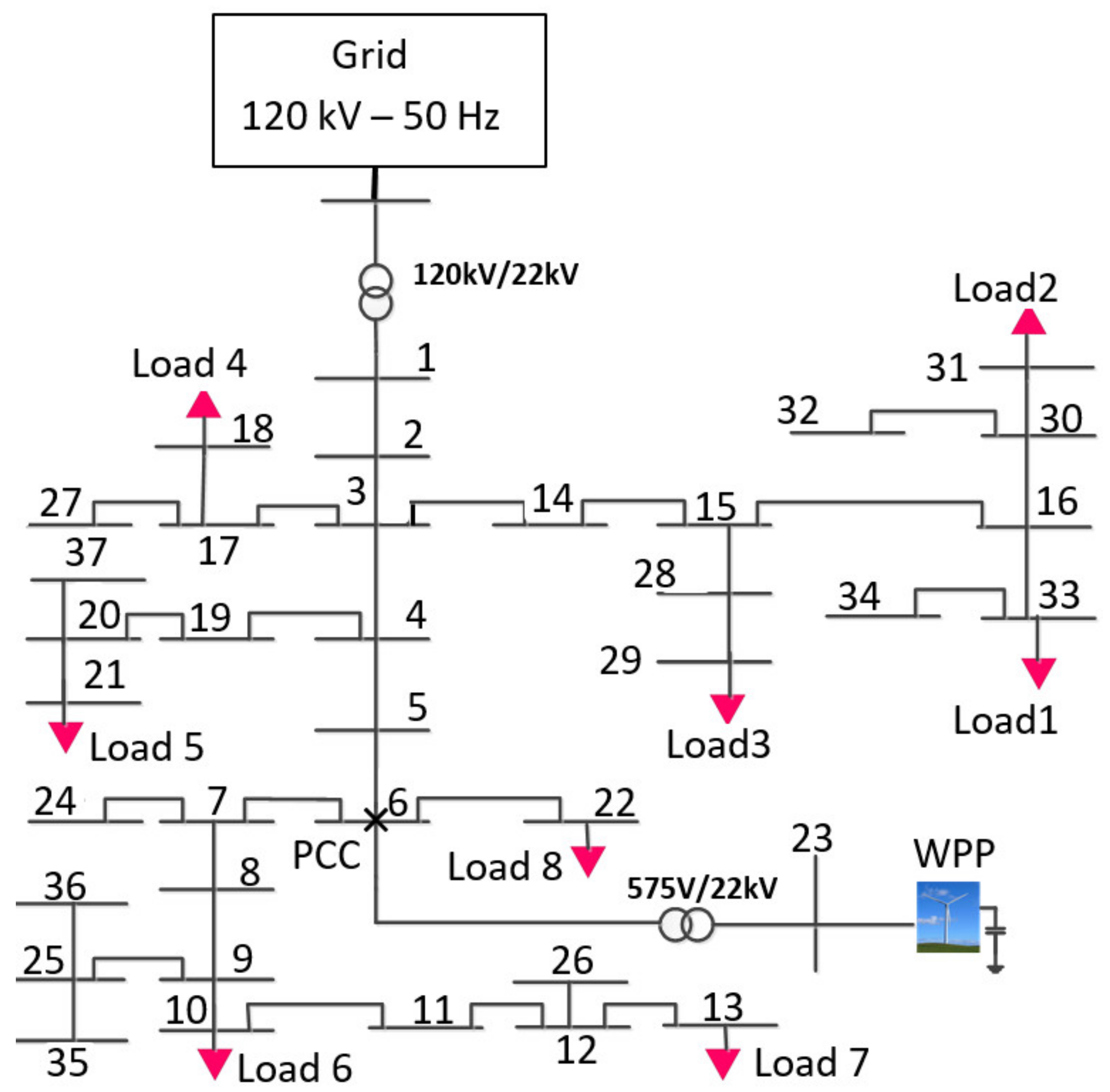
Figure 2.
9-bus test system.
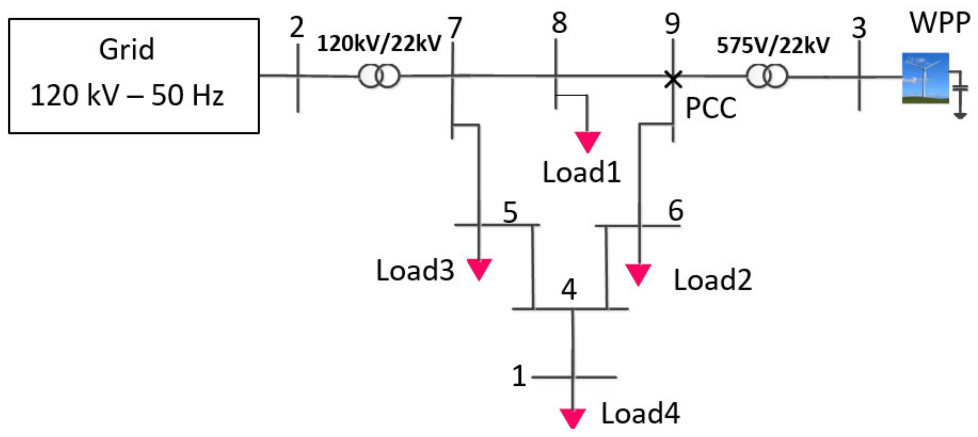
Figure 3.
VPCC-X/RPCC characteristic for each test system for both the Induction Generator (IG) and the Double Fed Induction Generator (DFIG).
Figure 3.
VPCC-X/RPCC characteristic for each test system for both the Induction Generator (IG) and the Double Fed Induction Generator (DFIG).
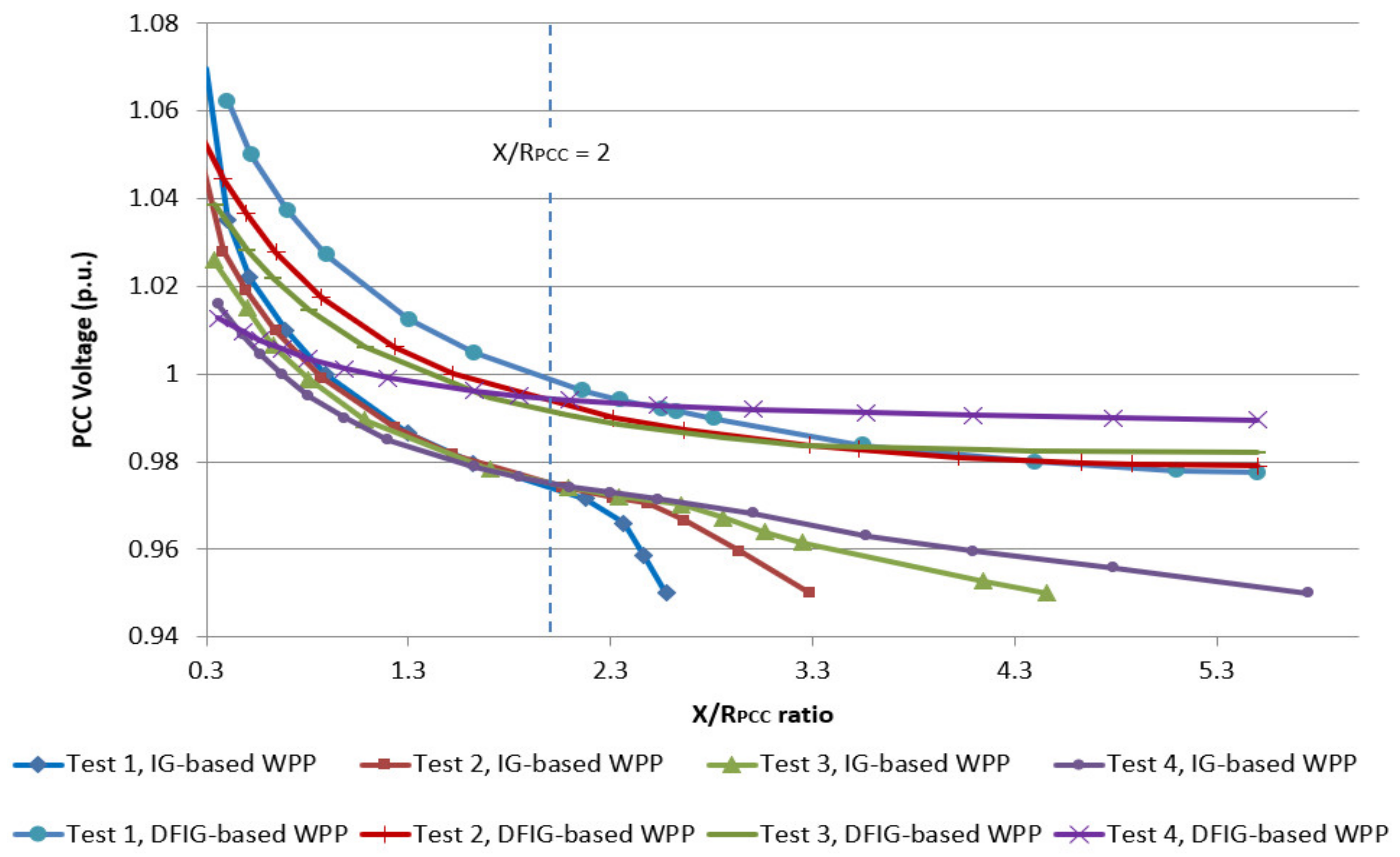
Figure 4.
General VPCC-X/RPCC characteristic curve given by (3) and (4) for different decay coefficients.
Figure 4.
General VPCC-X/RPCC characteristic curve given by (3) and (4) for different decay coefficients.
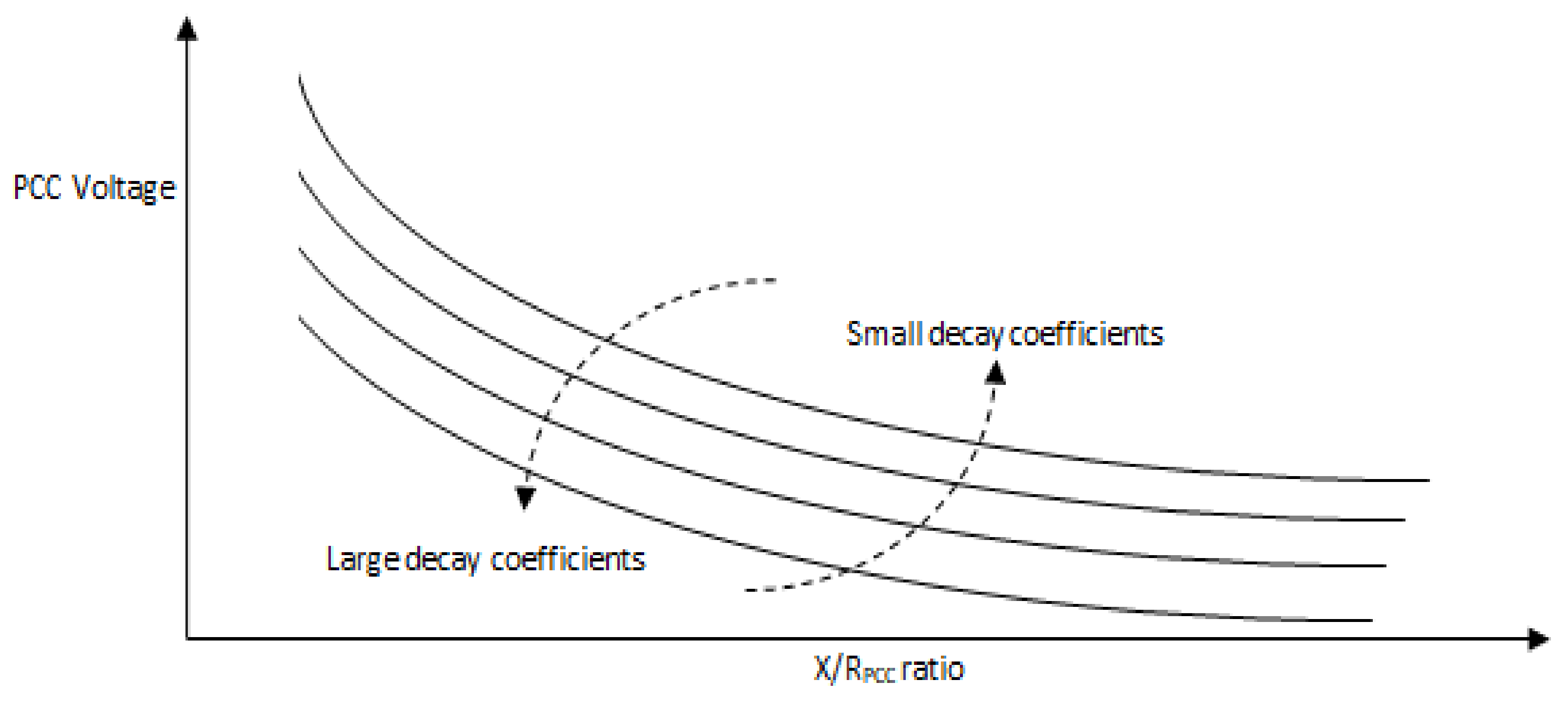
Figure 5.
Flowchart diagram of Func1.
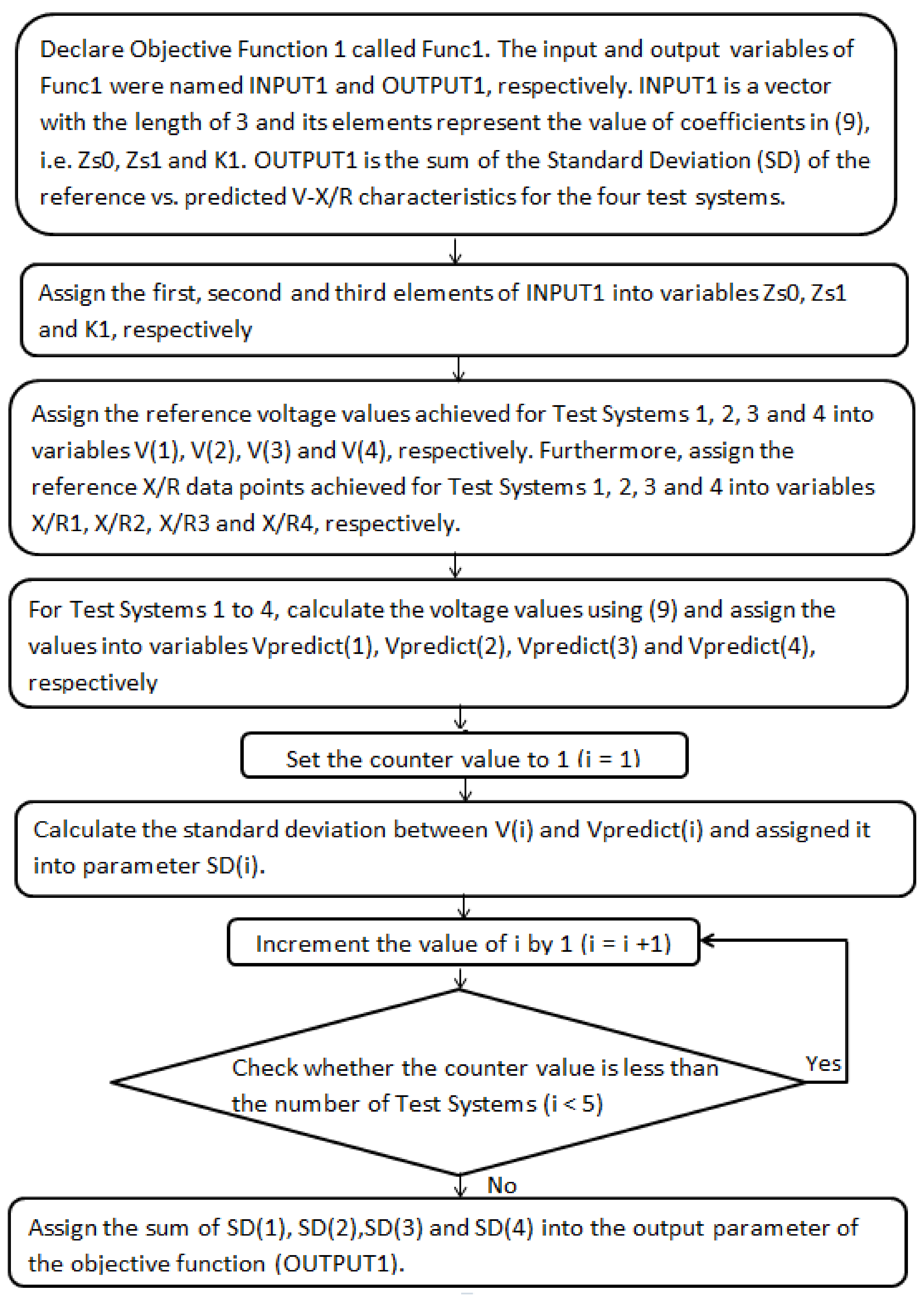
Figure 6.
VPCC-X/RPCC characteristics plotted by the developed alternative equations. (a) VPCC-X/RPCC curves obtained by (15) and (16) for Test 1; (b) VPCC-X/RPCC curves obtained by (15) and (16) for Test 2; (c) VPCC-X/RPCC curves obtained by (15) and (16) for Test 3; (d) VPCC-X/RPCC curves obtained by (15) and (16) for Test 4; (e) VPCC-X/RPCC curves obtained by (17) and (18) for Test 1; (f) VPCC-X/RPCC curves obtained by (17) and (18) for Test 2; (g) VPCC-X/RPCC curves obtained by (17) and (18) for Test 3; (h) VPCC-X/RPCC curves obtained by (17) and (18) for Test 4; (i) VPCC-X/RPCC curves obtained by (19) and (20) for Test 1; (j) VPCC-X/RPCC curves obtained by (19) and (20) for Test 2; (k) VPCC-X/RPCC curves obtained by (19) and (20) for Test 3; (l) VPCC-X/RPCC curves obtained by (19) and (20) for Test 4.

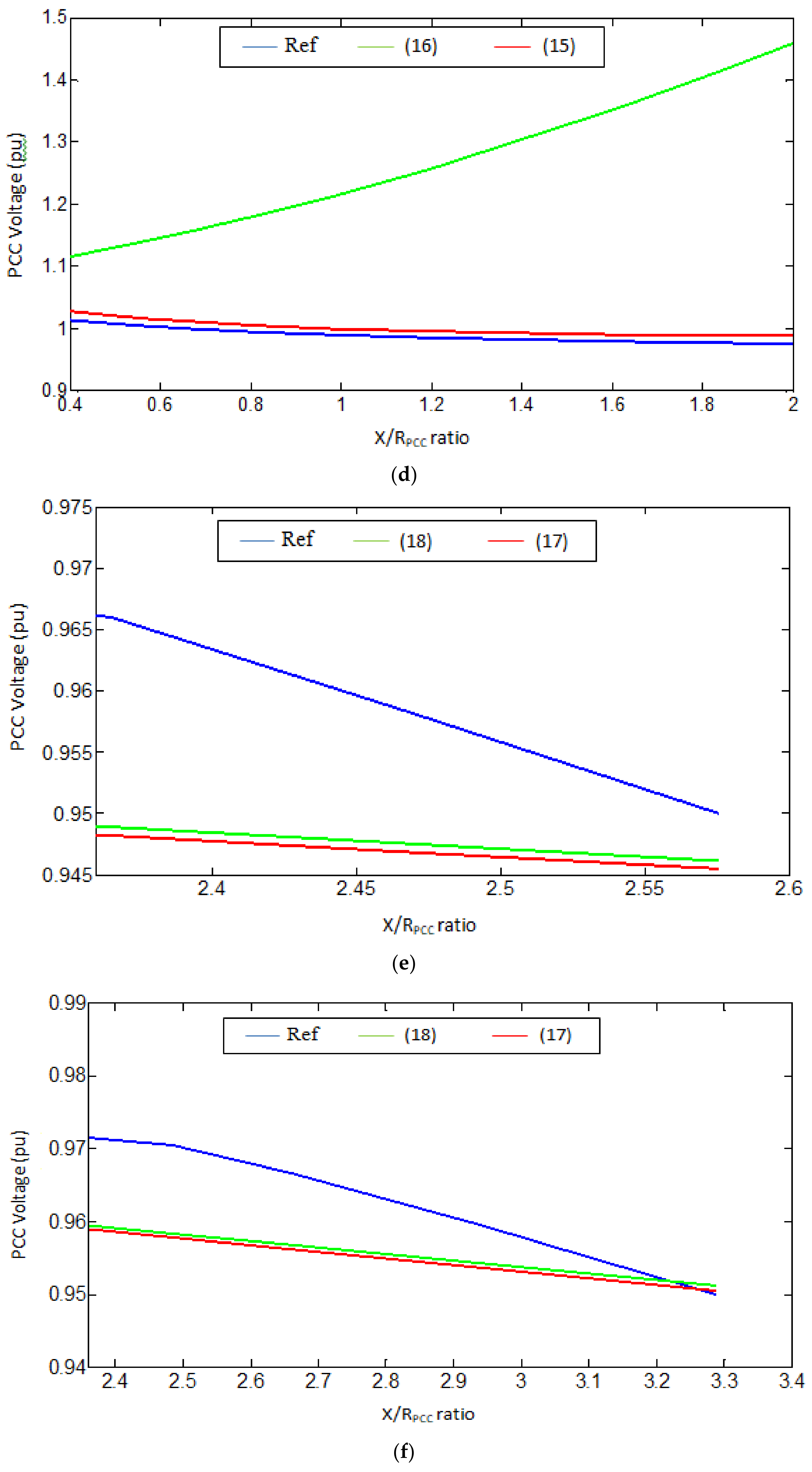
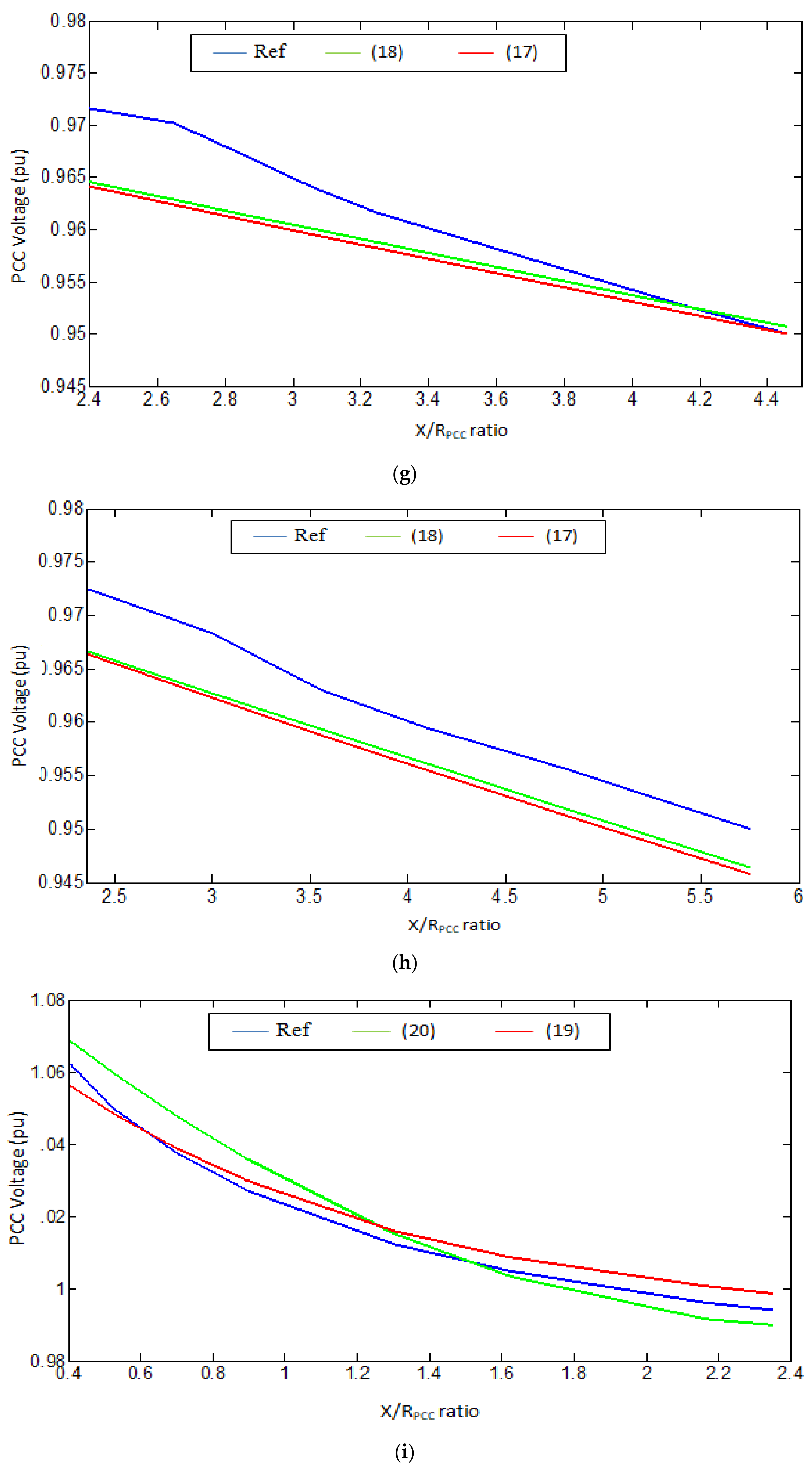
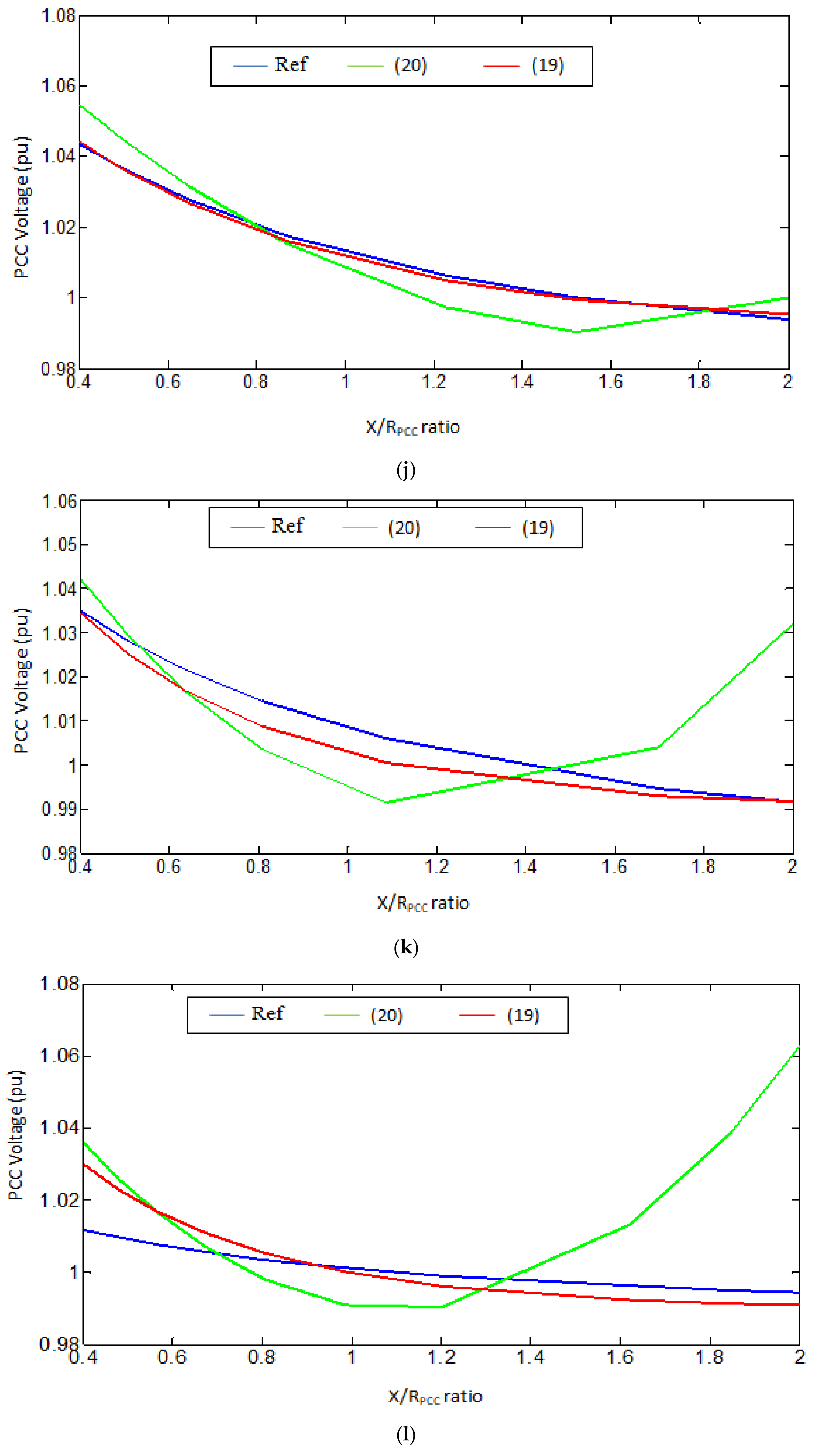
Figure 7.
Pwind versus VPCC characteristic for validation scenarios considered for the 9-bus and 37-bus test systems. (a) Scenario 1; (b) Scenario 2; (c) Scenario 3; (d) Scenario 4; (e) Scenario 5; (f) Scenario 6.
Figure 7.
Pwind versus VPCC characteristic for validation scenarios considered for the 9-bus and 37-bus test systems. (a) Scenario 1; (b) Scenario 2; (c) Scenario 3; (d) Scenario 4; (e) Scenario 5; (f) Scenario 6.
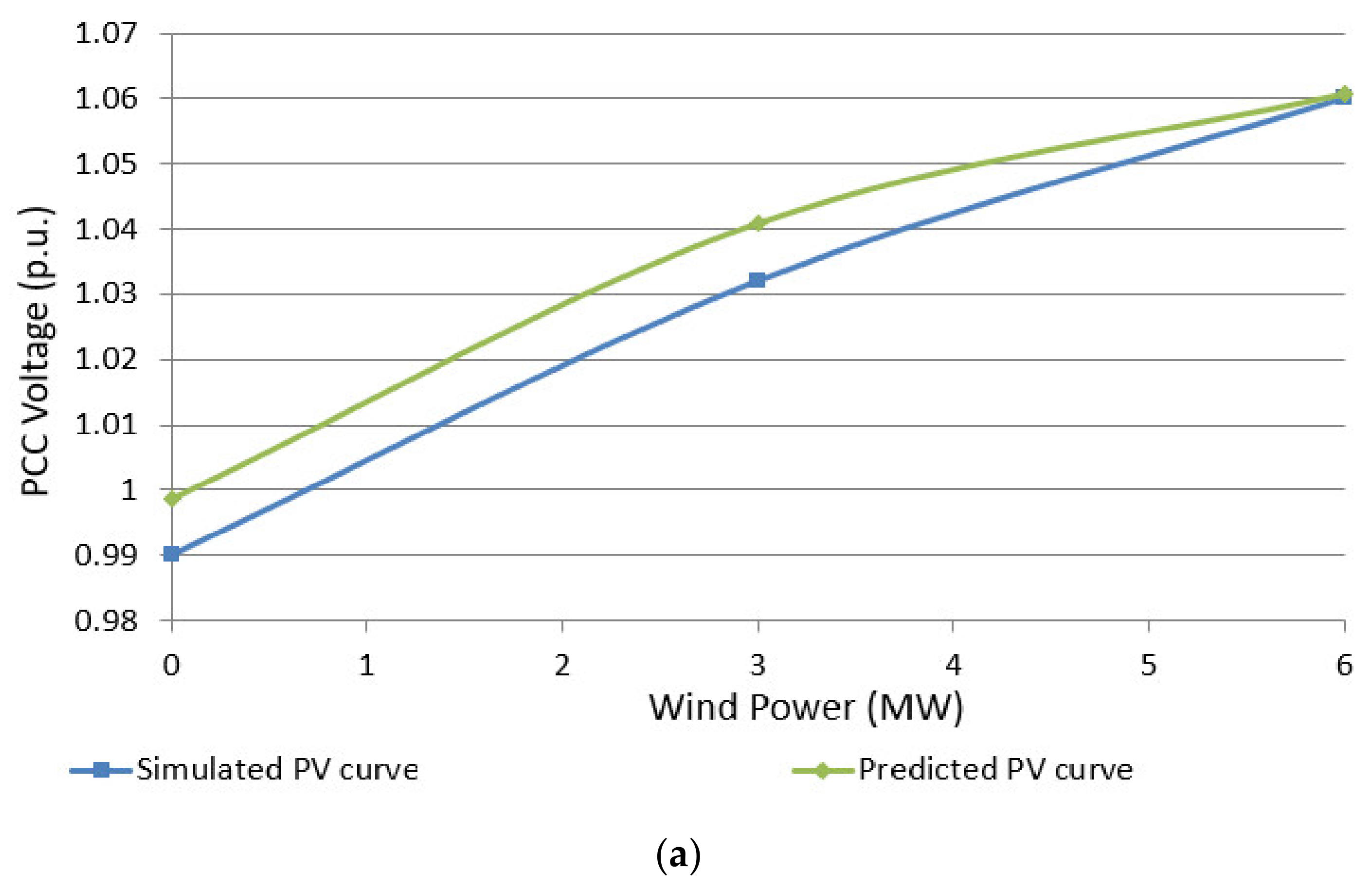
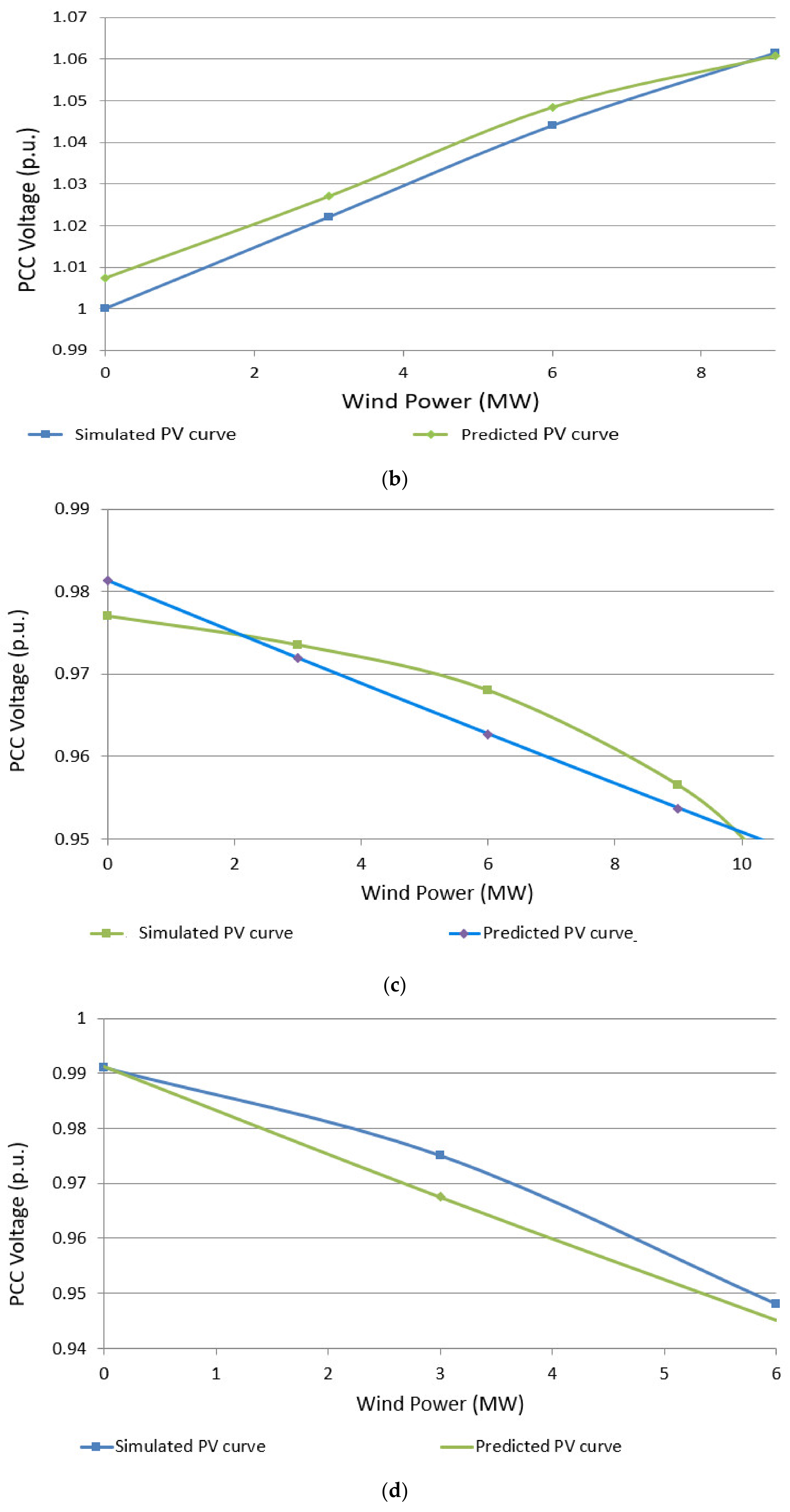
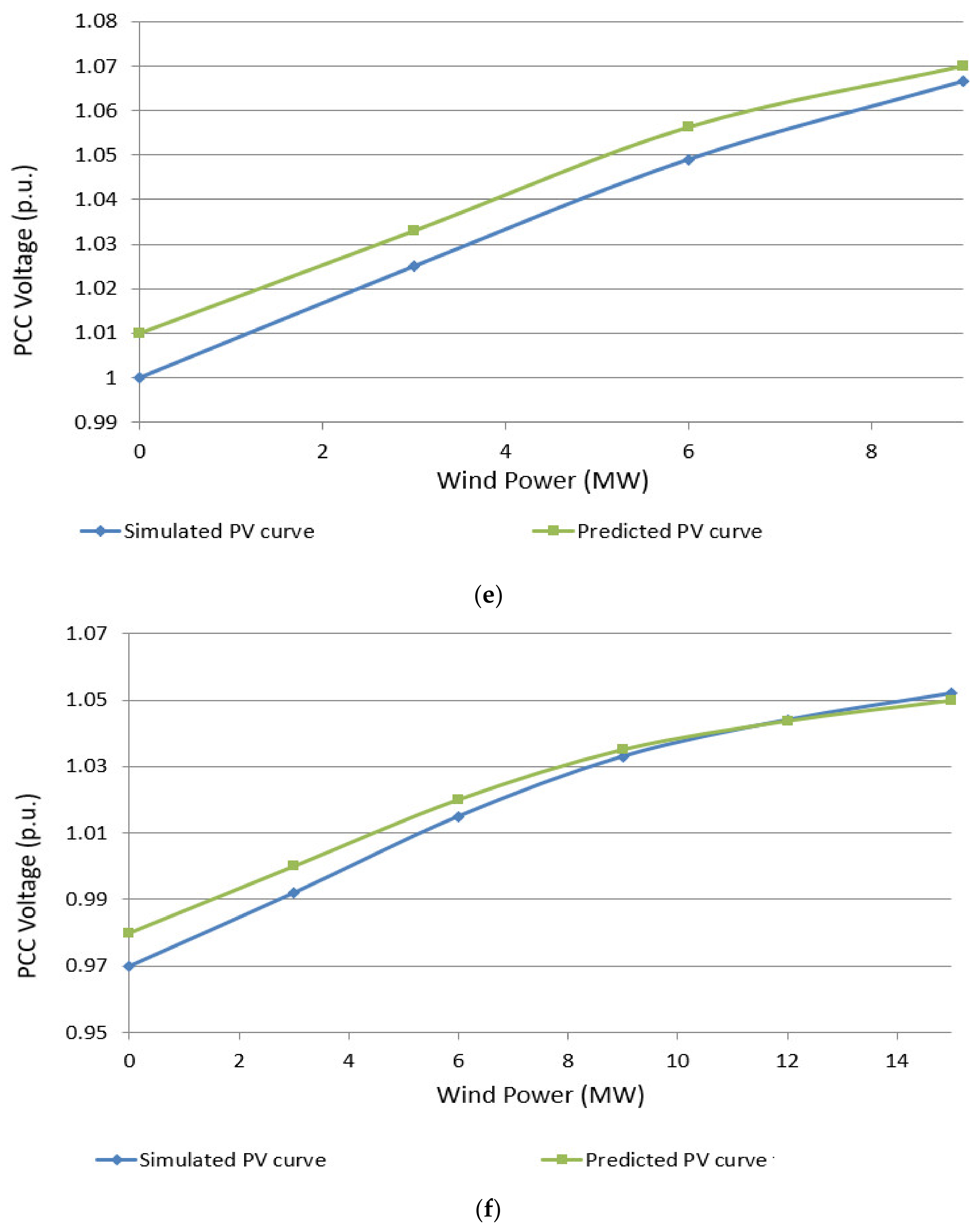
Figure 8.
Maximum permissible wind power generation ensuring 0.95 < VPCC < 1.05 for Scenarios 1 to 6.
Figure 8.
Maximum permissible wind power generation ensuring 0.95 < VPCC < 1.05 for Scenarios 1 to 6.
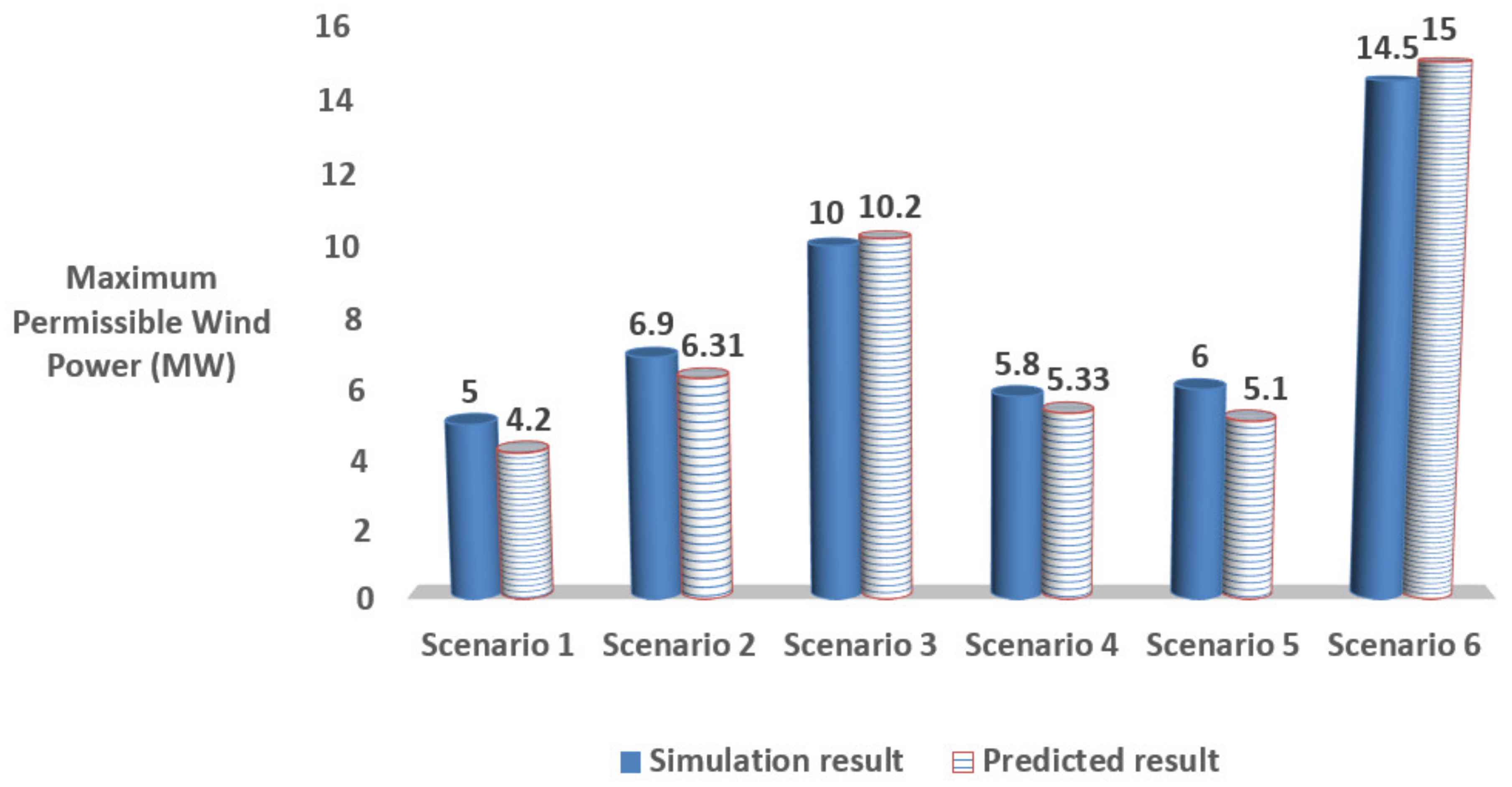
Figure 9.
30-bus test system.
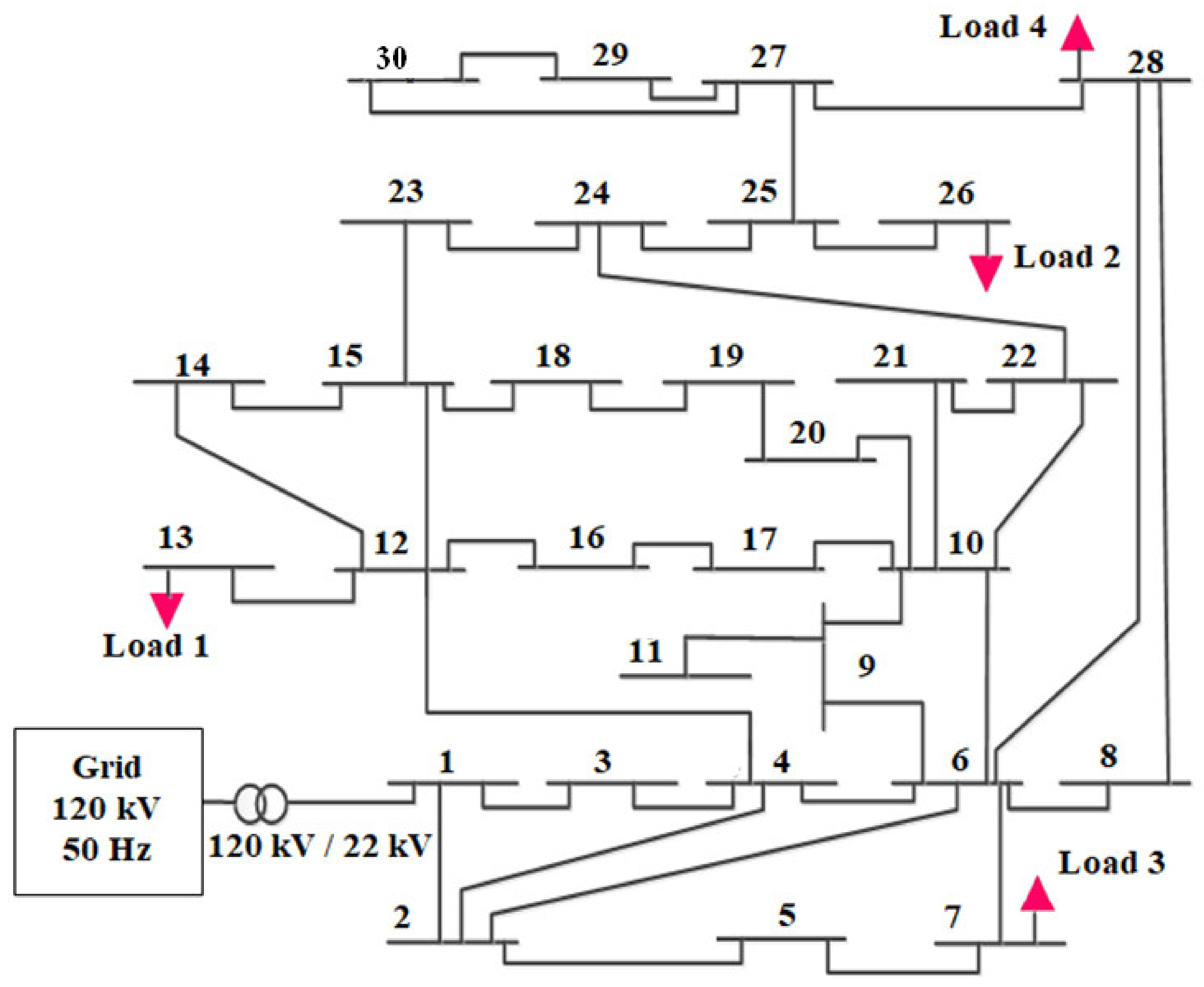
Figure 10.
Pwind versus VPCC curves for validation scenarios considered for the 30-bus test system. (a) Scenarios A and B; (b) Scenario C.
Figure 10.
Pwind versus VPCC curves for validation scenarios considered for the 30-bus test system. (a) Scenarios A and B; (b) Scenario C.
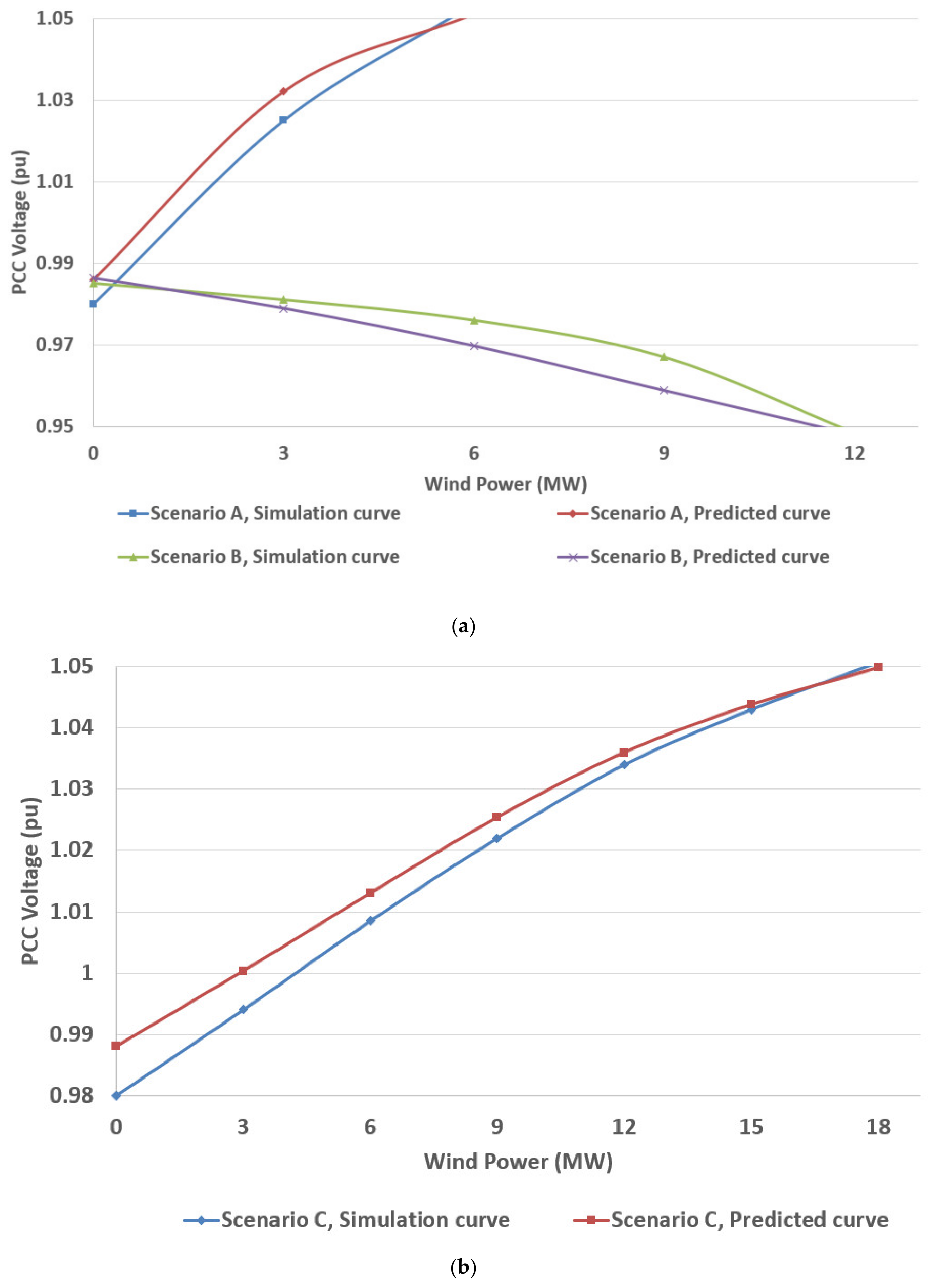
Figure 11.
Maximum permissible wind power generation ensuring 0.95 < VPCC < 1.05 for Scenarios A to C.
Figure 11.
Maximum permissible wind power generation ensuring 0.95 < VPCC < 1.05 for Scenarios A to C.
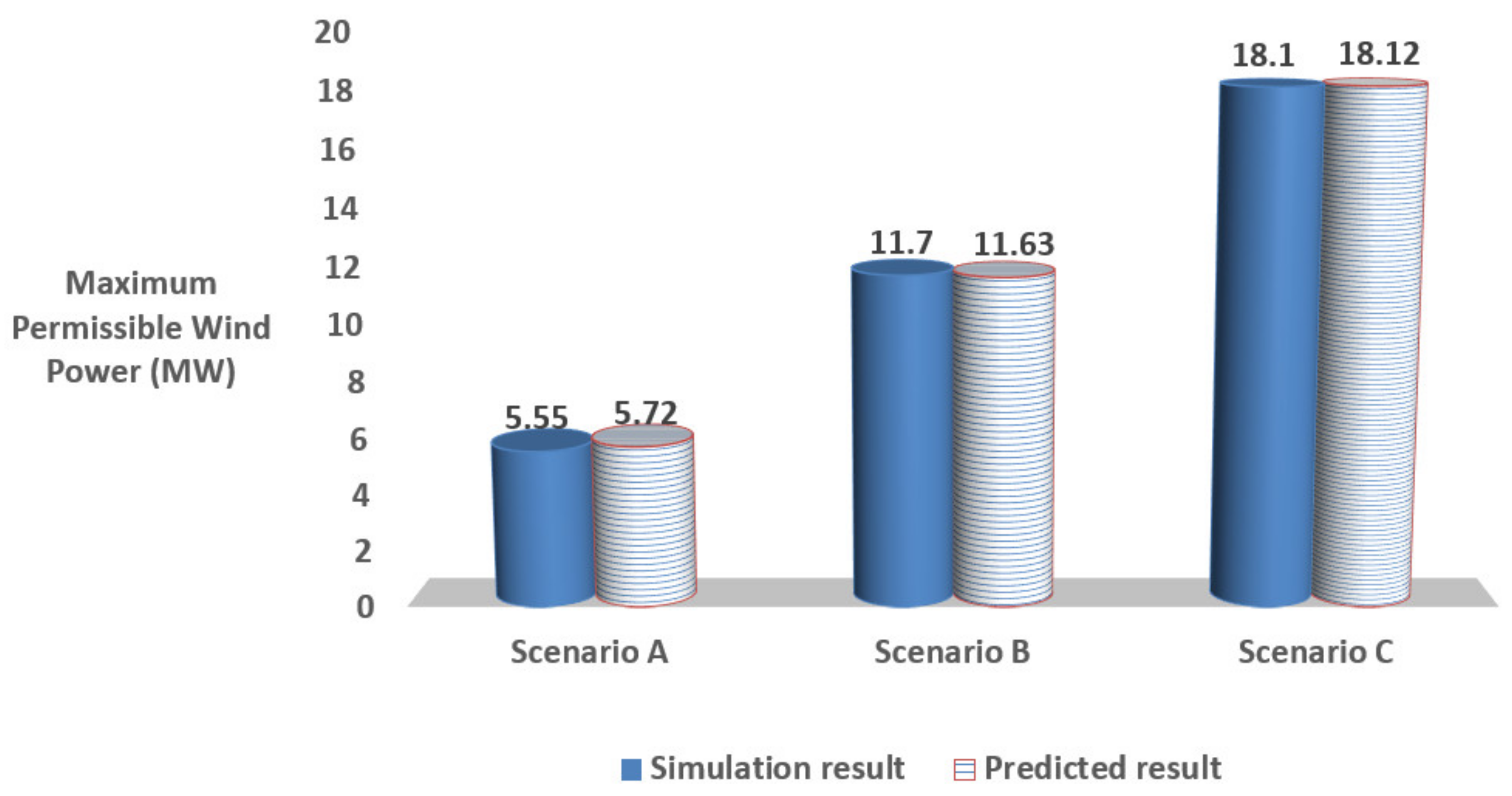
Table 1.
Point of Common Coupling (PCC) characteristics of each test system.
| Case Study | Topology | Isc (kA) | SCC (MVA) | Pwind (MW) | SCR |
|---|---|---|---|---|---|
| Test 1 | IEEE 37-bus system | 0.71 | 27 | 9 | 3 |
| Test 2 | IEEE 37-bus system | 1.05 | 40 | 9 | 4.5 |
| Test 3 | IEEE 9-bus system | 1.42 | 54 | 9 | 6 |
| Test 4 | IEEE 9-bus system | 0.55 | 21 | 3 | 7 |
Table 2.
Two main features considered for developing mathematical equations for IG-based Wind Power Plants (WPPs).
Table 2.
Two main features considered for developing mathematical equations for IG-based Wind Power Plants (WPPs).
| Feature | Description |
|---|---|
| Feature 1 | Voltage at feeders with a low X/RPCC ratio is increased as SCR is decreased. |
| Feature 2 | Voltage at feeders with a high X/RPCC ratio is decreased as SCR is decreased. |
Table 3.
Genetic Algorithm (GA) parameter settings.
| Parameter | Value/Type |
|---|---|
| Generation | 300 |
| population size | 200 |
| Selection | stochastic uniform |
| Crossover | Scattered |
| Mutation | constraint dependent |
Table 4.
Characteristics of the objective functions.
| Alternative Equation | Objective Function Name | Input of Objective Function | Output of Objective Function |
|---|---|---|---|
| (9) | Func1 | Coefficients of (9), i.e., Zs0, Zs1 and K1 | Error between the VPCC-X/RPCC graphs predicted by (9) and the reference curves presented in Figure 3 for IG-based WPP and X/RPCC < 2 |
| (10) | Func2 | Coefficients of (10), i.e., Ys0, Ys1 and Ys2 | Error between the VPCC-X/RPCC graphs predicted by (10) and the reference curves presented in Figure 3 for IG-based WPP and X/RPCC < 2 |
| (11) | Func3 | Coefficients of (11), i.e., Zl0, Zl1 and K3 | Error between the VPCC-X/RPCC graphs predicted by (11) and the reference curves presented in Figure 3 for IG-based WPP and X/RPCC > 2 |
| (12) | Func4 | Coefficients of (12), i.e., Yl0, Yl1 and Yl2 | Error between the VPCC-X/RPCC graphs predicted by (12) and the reference curves presented in Figure 3 for IG-based WPP and X/RPCC > 2 |
| (13) | Func5 | Coefficients of (13), i.e., Ws0, Ws1 and K5 | Error between the VPCC-X/RPCC graphs predicted by (13) and the reference curves presented in Figure 3 for DFIG-based WPP and X/RPCC < 2 |
| (14) | Func6 | Coefficients of (14), i.e., Us0, Us1 and Us2 | Error between the VPCC-X/RPCC graphs predicted by (14) and the reference curves presented in Figure 3 for DFIG-based WPP and X/RPCC < 2 |
Table 5.
Coefficients for Objective Functions 1 and 2.
| Coefficient | Zs0 | Zs1 | K1 | Ys0 | Ys1 | Ys2 |
| Value | 0.9867 | 0.0912 | 0.29 | 1.068 | 0.015 | 0.001 |
Table 6.
Coefficients for Objective Functions 3 and 4.
| Coefficient | Zl0 | Zl1 | K3 | Yl0 | Yl1 | Yl2 |
| Value | 0.788 | 0.195 | 0.24 | 0.9813 | 0.0427 | 0.002 |
Table 7.
Coefficients for Objective Functions 5 and 6.
| Coefficient | Ws0 | Ws1 | K5 | Us0 | Us1 | Us2 |
| Value | 0.99 | 0.101 | 0.347 | 1.102 | 0.03 | 0.002 |
Table 8.
Error between the reference VPCC-X/RPCC graphs and the graphs plotted by the alternative equations.
Table 8.
Error between the reference VPCC-X/RPCC graphs and the graphs plotted by the alternative equations.
| WPP Type | X/RPCC Range | Test System | Equation | SD | MAE | MRE |
|---|---|---|---|---|---|---|
| IG-based WPP | X/RPCC < 2 | 1 | 15 | 0.0264 | 0.026 | 0.0254 |
| - | - | - | 16 | 0.0324 | 0.0314 | 0.0305 |
| IG-based WPP | X/RPCC > 2 | 1 | 17 | 0.015 | 0.014 | 0.0144 |
| - | - | - | 18 | 0.0144 | 0.013 | 0.0137 |
| DFIG-based WPP | X/RPCC < 2 | 1 | 19 | 0.0038 | 0.0035 | 0.0034 |
| - | - | - | 20 | 0.0068 | 0.006 | 0.0058 |
| IG-based WPP | X/RPCC < 2 | 2 | 15 | 0.0155 | 0.0145 | 0.0143 |
| - | - | - | 16 | 0.0247 | 0.0223 | 0.0218 |
| IG-based WPP | X/RPCC > 2 | 2 | 17 | 0.0102 | 0.0091 | 0.0095 |
| - | - | - | 18 | 0.0097 | 0.0087 | 0.0091 |
| DFIG-based WPP | X/RPCC < 2 | 2 | 19 | 0.0014 | 0.0012 | 0.0012 |
| - | - | - | 20 | 0.0103 | 0.0093 | 0.009 |
| IG-based WPP | X/RPCC < 2 | 3 | 15 | 0.0117 | 0.0116 | 0.0115 |
| - | - | - | 16 | 0.0318 | 0.0274 | 0.0267 |
| IG-based WPP | X/RPCC > 2 | 3 | 17 | 0.0055 | 0.0047 | 0.0049 |
| - | - | - | 18 | 0.0052 | 0.0044 | 0.0046 |
| DFIG-based WPP | X/RPCC < 2 | 3 | 19 | 0.0036 | 0.0031 | 0.003 |
| - | - | - | 20 | 0.0361 | 0.0234 | 0.0223 |
| IG-based WPP | X/RPCC < 2 | 4 | 15 | 0.0122 | 0.0121 | 0.012 |
| - | - | - | 16 | 0.2876 | 0.2523 | 0.194 |
| IG-based WPP | X/RPCC > 2 | 4 | 17 | 0.0051 | 0.005 | 0.0052 |
| - | - | - | 18 | 0.0046 | 0.0045 | 0.0047 |
| DFIG-based WPP | X/RPCC < 2 | 4 | 19 | 0.0088 | 0.0065 | 0.0064 |
| - | - | - | 20 | 0.0327 | 0.0225 | 0.0215 |
Table 9.
Best fit functions considering WPP type and X/RPCC range.
| WPP Type | X/RPCC Range | Proposed Equation |
|---|---|---|
| IG-based WPP | X/RPCC < 2 | (15) |
| IG-based WPP | X/RPCC > 2 | (18) |
| DFIG-based WPP | X/RPCC < 2 | (19) |
Table 10.
Proposed mathematical model.
| Equation | Equation Number | Application |
|---|---|---|
| Plotting PV curve for IG WPP with X/RPCC < 2. | ||
| Plotting PV curve for IG WPP with X/RPCC > 2. | ||
| Plotting PV curve for DFIG WPP with X/RPCC < 2 | ||
| IG WPP sizing with X/RPCC < 2 | ||
| IG WPP sizing with X/RPCC > 2 | ||
| DFIG WPP sizing with X/RPCC < 2 | ||
Table 11.
ΔVPCC obtained by (24) and (26) for X/RPCC = 0.5 and SCR = 2.5.
| WPP Type | SCR | X/RPCC | Proposed Equation | ΔVPCC (%) |
|---|---|---|---|---|
| IG-based WPP | 2.5 | 0.5 | (24) | 7 |
| DFIG-based WPP | 2.5 | 0.5 | (26) | 7.5 |
Table 12.
Parameters considered for validation scenarios used in Case study 1.
| Scenario | WPP Type | Test System | Topology | SCC (MVA) | X/RPCC | Vinitial |
|---|---|---|---|---|---|---|
| 1 | IG-based WPP | Test 1 | IEEE 37-bus system | 27 | 0.3 | 0.99 |
| 2 | IG-based WPP | Test 3 | IEEE 9-bus system | 54 | 0.3 | 1 |
| 3 | IG-based WPP | Test 2 | IEEE 37-bus system | 40 | 3 | 0.98 |
| 4 | IG-based WPP | Test 4 | IEEE 9-bus system | 21 | 4 | 0.99 |
| 5 | DFIG-based WPP | Test 1 | IEEE 37-bus system | 27 | 0.5 | 1 |
| 6 | DFIG-based WPP | Test 2 | IEEE 37-bus system | 40 | 0.4 | 0.97 |
Table 13.
WPP type, PCC site and parameters in scenarios considered for the 30-bus system.
| Scenario | WPP Type | PCC Bus | SCC (MVA) | X/RPCC | Vinitial |
|---|---|---|---|---|---|
| A | IG-based WPP | Bus 26 | 18 | 0.4 | 0.98 |
| B | IG-based WPP | Bus 13 | 46 | 3.5 | 0.985 |
| C | DFIG-based WPP | Bus 7 | 68 | 0.4 | 0.98 |
© 2020 by the authors. Licensee MDPI, Basel, Switzerland. This article is an open access article distributed under the terms and conditions of the Creative Commons Attribution (CC BY) license (http://creativecommons.org/licenses/by/4.0/).
Share and Cite
MDPI and ACS Style
Alizadeh, S.M.; Sadeghipour, S.; Ozansoy, C.; Kalam, A. Developing a Mathematical Model for Wind Power Plant Siting and Sizing in Distribution Networks. Energies 2020, 13, 3485. https://doi.org/10.3390/en13133485
AMA Style
Alizadeh SM, Sadeghipour S, Ozansoy C, Kalam A. Developing a Mathematical Model for Wind Power Plant Siting and Sizing in Distribution Networks. Energies. 2020; 13(13):3485. https://doi.org/10.3390/en13133485
Chicago/Turabian StyleAlizadeh, Seyed Morteza, Sakineh Sadeghipour, Cagil Ozansoy, and Akhtar Kalam. 2020. "Developing a Mathematical Model for Wind Power Plant Siting and Sizing in Distribution Networks" Energies 13, no. 13: 3485. https://doi.org/10.3390/en13133485
Note that from the first issue of 2016, this journal uses article numbers instead of page numbers. See further details here.