Interval Optimization-Based Optimal Design of Distributed Energy Resource Systems under Uncertainties

Abstract

Distributed energy resource (DER) systems have elicited increasing attention and applications because of their excellent economic and environmental performance. However, uncertainties exist in such systems, preventing their potential advantages to be realized. In this study, an interval optimization-based model for the optimal design of DER systems is proposed, considering uncertainties in energy prices, renewable energy intensity, and load demands. Uncertainties are described as interval numbers, and the uncertain optimization model is transformed into a deterministic optimization problem using the order relationship and probability degree of interval numbers. The proposed model is applied to a typical hospital in Lianyungang, China, and its effectiveness is verified. One deterministic case and three uncertain cases are designed. The effects of uncertainties on system configuration and economic performance are also analyzed, and the optimal operation strategy under the three uncertainties is determined. A sensitivity analysis is conducted to analyze the effects of probability degree and weighting coefficient on total annual cost. Results show that uncertainties exert a cumulative effect on system optimization outcomes, and the proposed interval optimization model can obtain robust solutions to uncertainties.

1. Introduction

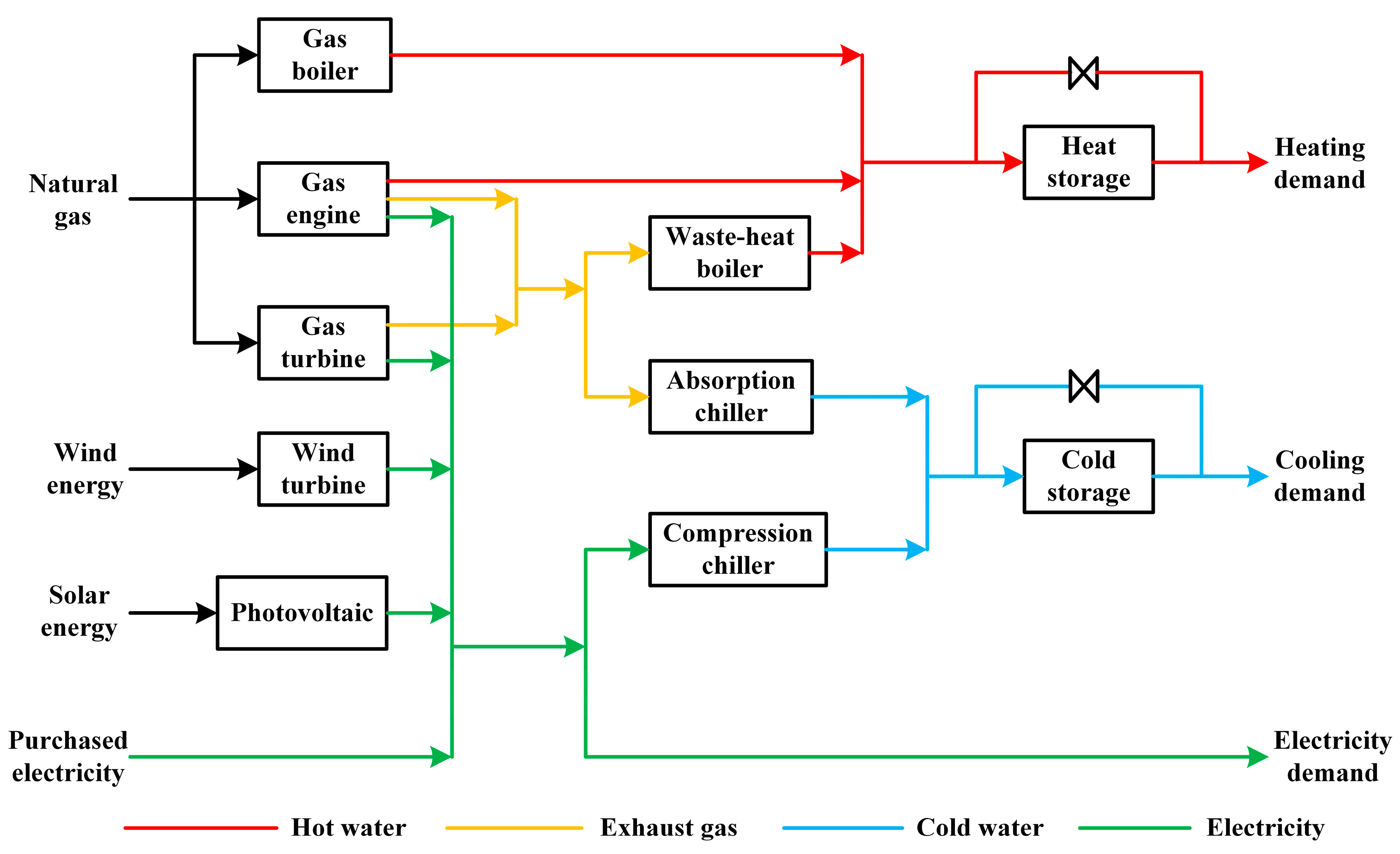
Distributed energy resource (DER) systems have elicited increasing attention and applications to save energy resources, reduce carbon emissions, and lessen energy costs. DER systems can utilize multiple energy forms (e.g., traditional energy and renewable energy), incorporate various types of equipment (e.g., gas engines, boilers, chillers, and storage units), and provide different forms of energy to end users (e.g., electricity, cooling, and heating). Through on-site generation and the reuse of exhaust heat, DER systems provide a series of advantages, such as low energy transmission losses, high efficiency, and excellent economic and environmental performance [1].

The design of DER system configuration and operation strategy is difficult because of the complex structure, numerous pieces of equipment, long operating period, and various energy forms of such systems. In this context, optimization models have been proposed for the optimal design of DER systems. The optimization of DER systems has been conducted from different aspects, such as exergy [2,3], multi-objective [4,5], design [2,6,7], and operation [8,9] optimization. In these studies, however, mathematical models were proposed in a deterministic environment without considering uncertainties. In application, these systems are impacted by many uncertainties, such as those in energy prices, renewable energy intensity, energy demands of end users, and interest rates [10]. Without considering such uncertainties, the results obtained may be suboptimal and the designed benefits of DER systems may not be realized [11]. Therefore, optimization methods that can incorporate uncertainties into the system design process should be adopted [12].

Stochastic optimization (SO) is an effective method that can address optimization problems with uncertainties. Uncertainties in SO are described with probability distribution or scenarios with probability [13]. Moreover, multistage SO has been developed in the optimal design of DER systems [11,14,15,16]. Mavromatidis et al. [11] formulated a two-stage stochastic programming model for the optimal design of distributed energy systems; this model considers uncertainties in energy carrier prices, emission factors, energy demands, and incoming solar radiation patterns. Beraldi et al. [14] proposed an optimal management model for DER systems under uncertainties in demand profiles, electricity prices, and renewable sources using two-stage stochastic programming.

Robust optimization (RO) is another widely used method that can deal with uncertainties. Uncertainties are distributed in uncertainty sets in RO. The purpose of RO is to find a solution that satisfies the constraints for all possible situations and optimizes the objective function value in the worst-case scenario [17]. RO has been applied to the optimization of energy systems under uncertainties [18,19,20,21]. Wang et al. [18] proposed an RO-based risk-averse energy transaction approach that considers uncertainties in renewable energy and transaction prices in networked microgrids. Jeddi et al. [19] constructed an optimization model for DER planning that considers load uncertainty with a RO approach.

In the preceding studies, the probability distribution function, probability scenarios, or uncertainty sets are introduced when applying SO and RO to the optimal design of DER systems to describe uncertainties and solve problems. However, this additional information will complicate the optimization process. In addition, such information is typically based on a huge amount of historical data that are difficult to obtain, particularly when the system is applied to a new area or object. Moreover, some uncertainties in DER systems cannot be accurately described as a probability distribution function. Interval optimization, which was proposed by Moore [22], is an uncertainty optimization theory that considers situations in which uncertainties change by following a specific interval.

Comparing with SO and RO, interval optimization has advantages in the following aspects. First, in this optimization approach, knowledge is only required of the lower and upper limits of uncertain variables, which can be easier to obtain in practice than the probability distribution function. In addition, interval optimization can be easily implemented and can provide quicker solutions. Moreover, the attitude of interval optimization toward risks is neutral, and it can obtain less conservative results than RO, which is pessimistic toward risks and optimizes problems on the basis of the worst-case scenario. In interval optimization, the interval of the objective function is optimized rather than the expected value of the objective such as in SO and RO, helping decision makers identify the range in which the possible solution may fall. Additionally, the parameters defined in the formulation and solution processes in interval optimization, such as probability degree and weighting coefficient, can be selected appropriately to meet various requirements in accordance with the attitude of decision makers toward risks and actual conditions. The drawback of interval optimization is that it cannot provide the importance and occurrence probability of results in the interval because of the simple uncertainty information in input parameters. Interval optimization has been applied to the uncertain optimization of various energy systems, such as household multi-energy [23,24], hybrid energy [25], and gas–electricity integrated energy [26,27,28] systems. The results show that interval optimization can effectively handle uncertainties in energy systems and obtain robust solutions to uncertainties.

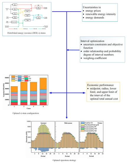
In the current study, an interval optimization model for the optimal design of DER systems under uncertainties is constructed. Compared to the previous work, the contributions of this work primarily lie in three aspects. First, an interval optimization model is developed for the optimal design of DER systems under uncertainties, which can effectively overcome the shortcomings of SO and RO as discussed above. To the best of our knowledge, this is the first time that interval optimization has been incorporated into the optimal design of DER systems. Second, the major uncertainties (uncertainties in energy prices, renewable energy intensity, and load demands) in DER systems are considered, thus allowing complex uncertain situations to be handled and more accurate results to be obtained. Third, the analysis of the effects of uncertainties on the DER systems is more comprehensive than some closely related references such as [15,29]. The configuration, economic performance, and operation strategy of DER systems under uncertainties are analyzed, and the effects of uncertainties are highlighted by comparing the results of uncertain cases to that of deterministic case.

The remainder of the paper is arranged as follows. After the introduction section, Section 2 presents the mathematical models for the deterministic mixed-integer linear programming (MILP) model, interval optimization, and the interval optimization model for DER systems. Section 3 describes the numerical study. Section 4 introduces the setting of the cases. The results and analysis are presented in Section 5. Lastly, the conclusion is provided in Section 6.

2. Mathematic Models

2.1. Deterministic MILP Model

In the DER system considered in this work, the power generation equipment includes a gas engine (GE) and gas turbine (GT), which use natural gas as an energy source, and a photovoltaic (PV) system and wind turbine (WT), which use renewable energy (solar energy and wind energy, respectively). A waste-heat boiler (WB) and absorption chiller (AC) reuse energy in exhaust gas from the GE and the GT. A gas boiler (GB) and compression chiller (CC) use natural gas and electricity to produce hot and cold water, respectively. Heat storage (HS) and cold storage (CS) can store and release hot and cold water, respectively, and adjust energy flow in the system. Figure 1 shows the superstructure of the considered DER system.

In the optimization model, the objective is to minimize the total annual cost C_Total, which is the sum of the equipment capital investment cost C_ECapital, energy cost C_Energy, and operating and maintenance cost of the equipment C_EOM, and then subtract the renewable energy subsidy R_subsidy, as follows:

$$C_{\mathrm{Total}}=C_{\mathrm{ECapital}}+C_{\mathrm{Energy}}+C_{\mathrm{EOM}}-R_{\mathrm{subsidy}}$$

(1)

Energy cost is the product of energy prices EPrice_u of energy form u, the amount of energy purchased EPG_k,u at time k, and annual duration hours AH_k.

$$C_{Energy}={\displaystyle \sum _{k\in K}{\displaystyle \sum _{u\in U}EPric{e}_u\times EP{G}_{k,u}\times A{H}_k}}$$

(2)

The model contains three types of constraints. The first category of constraints is the selected number and capacity of pieces of equipment. The selected number n_i,j of equipment type i with capacity j cannot exceed its maximum available number N_i,j. γ_i,j is a binary variable that denotes whether equipment type i with capacity j is selected (0 for not selected, 1 for selected). Each equipment type can choose only one type of capacity.

$$\begin{array}{l}\{\begin{array}{l}{n}_{i,j_i}\le N_{i,j_i}\times {\gamma }_{i,j_i}\\ {\gamma }_{i,j_i}\le n_{i,j_i}\end{array}\hspace{0.17em}\hspace{0.17em}\forall i\in I,j_i\in J_i\\ {\displaystyle \sum _{j_i\in J_i}{\gamma }_{i,j_i}}\le 1\hspace{0.17em}\hspace{0.17em}\forall i\in I\end{array}$$

(3)

The second category of constraints is the operation characteristics of equipment. For the equipment that utilizes renewable energy (e.g., WT and PV), the generated energy y_k,RE,el is dependent on the surface area of the installed equipment WArea_jRE, renewable energy intensity Intens_k,RE, generation efficiency η_jRE, and the number of pieces of operating equipment δ_k,RE. Meanwhile, the generated electricity cannot exceed the rated capacity Rcap_RE,jRE of the operating equipment.

$$y_{k,RE,el}\le {\displaystyle \sum _{j_{RE}\in J_{RE}}WAre{a}_{j_{RE}}\times Inten{s}_{k,RE}\times {\eta }_{j_{RE}}\times {\gamma }_{RE,j_{RE}}\times {\delta }_{k,RE}}\begin{array}{cc}& \end{array}\forall k\in K$$

(4)

$$y_{k,RE,el}\le {\displaystyle \sum _{j_{RE}\in J_{RE}}Rca{p}_{RE,j_{RE}}\times {\gamma }_{RE,j_{RE}}\times {\delta }_{k,RE}} \forall k\in K$$

(5)

The third category of constraints is the energy balance in the system. The sum of the energy produced by equipment y_k,i,u and the purchased energy should not be smaller than the sum of the load demands LD_k,u of end users, energy consumption of equipment x_k,u, and energy flow in storage E_k,u.

$${\displaystyle \sum _i{y}_{k,i,u}}+EP{G}_{k,u}\ge L{D}_{k,u}+x_{k,u}+E_{k,u}\begin{array}{cc}& \end{array}\forall k\in K$$

(6)

A more detailed configuration of the deterministic mathematical model for the optimal design of DER systems can be found in our previous work [29].

2.2. Interval Optimization

An interval number A^I represents a random variable that is distributed between the lower limit A^L and the upper limit A^R. It can be expressed as:

$$A^I=[A^L,A^R]=\left\{x|A^L\le x\le A^R,x\in R\right\}$$

(7)

When A^L = A^R, the interval number degenerates to a real number. The interval number can also be expressed as:

$$A^I=\langle A^c,A^w\rangle =\left\{x|A^c-A^w\le x\le A^c+A^w\right\}$$

(8)

where A^c and A^w are the midpoint and radius values of the interval number, which can be expressed as:

$$A^c=\frac{A^R+A^L}{2},A^w=\frac{A^R-A^L}{2}$$

(9)

The mathematical programming model with interval numbers can be expressed as:

$$\begin{array}{l}\underset{X}{\min }f(X,U)\\ s.t. g_i(X,U)\le (=,\ge )b_i^I=[b_i^L,b_i^R],i=1,2,\dots l,X\in {\Omega }^n\\ U\in U^I=[U^L,U^R],U_i\in U_i^I=[U_i^L,U_i^R],i=1,2,\dots ,q\end{array}$$

(10)

where f and g_i are the objective function and constraints that contain interval uncertainties, respectively; and X and U are the decision variables and interval uncertainties, respectively. $b_i^I$ is the right-hand side interval of the ith constraint, and l is the number of the constraints. Ωⁿ is the range of X, and q is the dimension of U.

The preceding mathematical model cannot be solved directly because of the existence of interval number uncertainties.

The probability degree of interval numbers can be used to compare interval numbers A^I and B^I, and their formulations are discussed in a previous work [30]. When interval number B^I degenerates into a real number b, the probability degree of A^I ≤ b is expressed as:

$$P(A^I\le b)=\{\begin{array}{l}0,b\le A^L\\ \frac{b-A^L}{A^R-A^L},A^L<b\le A^R\\ 1,b>A^R\end{array}$$

(11)

When interval number A^I degenerates into a real number a, the probability degree of a ≤ B^I is expressed as:

$$P(a\le B^I)=\{\begin{array}{l}1,\mathrm{a}\le B^L\\ \frac{B^R-a}{B^R-B^L},B^L<a\le B^R\\ 0,\mathrm{a}>B^R\end{array}$$

(12)

By utilizing the probability degree, the uncertainty constraints with the form of ≤, such as g_i(X,U) ≤ $b_i^I$, can be transformed into a deterministic constraint as follows:

$$P(g_i^I(X)\le b_i^I)\ge {\lambda }_i,$$

(13)

where $0\le \lambda \le 1$ is the predefined probability degree level, representing the probability that the constraint is satisfied. $g_i^I\left(X\right)$ is the possible interval of the uncertain constraint $g_i^I\left(X,U\right)$, as follows:

$$g_i^I(X)=[g_i^L(X),g_i^R(X)]$$

(14)

The lower limit $g_i^L\left(X\right)$ and the upper limit $g_i^R\left(X\right)$ of interval $g_i^I\left(X\right)$ can be obtained using:

$$g_i^L(X)=\underset{U}{\min }{g}_i(X,U),g_i^R(X)=\underset{U}{\max }{g}_i(X,U)$$

(15)

The uncertain constraints with the form of ≥, such as g_i(X,U) ≥ $b_i^I$, can be easily transformed into the form of ≤, such as $b_i^I$ ≤ g_i(X,U), and further transformed into the deterministic form using the aforementioned method.

Given the existence of interval uncertainties U, the possible value of the objective function f(X,U) will fall within an interval:

$$f^I(X)=[f^L(X),f^R(X)]=\langle f^c(X),f^w(X)\rangle$$

(16)

The midpoint f^c(X) and radius f^w(X) of the objective interval f^I(X) are defined as:

$$f^c(X)=\frac{f^L(X)+f^R(X)}{2},f^w(X)=\frac{f^R(X)-f^L(X)}{2}$$

(17)

The lower limit f^L(X) and upper limit f^R(X) of the objective interval can be obtained using:

$$f^L(X)=\underset{U}{\min }f(X,U),f^R(X)=\underset{U}{\max }f(X,U)$$

(18)

Using the order relationship of interval numbers, the minimum objective function in Equation (10) is converted to minimize the midpoint and radius of the interval objective value [31]:

$$\underset{X}{\min }\left(f^c(X),f^w(X)\right)$$

(19)

A weighting coefficient β between 0 and 1 is adopted to transform the preceding multi-objective problem into the following single-objective optimization problem:

$$\underset{X}{\min }f(X)=(1-\beta )f^c(X)+\beta f^w(X)$$

(20)

Through the aforementioned method, the uncertain interval optimization problem with uncertain constraints and objective function is transformed into a deterministic optimization problem and can be solved using conventional mathematical programming solvers.

2.3. Interval Optimization Model for DER Systems

After considering uncertainties, renewable energy intensity becomes an interval number $Intens\begin{array}{c}I\\ k,RE\end{array}$ with lower limit $Intens\begin{array}{c}L\\ k,RE\end{array}$ and upper limit $Intens\begin{array}{c}R\\ k,RE\end{array}$, and the uncertain constraint with renewable energy intensity becomes:

$$y_{k,RE,el}\le {\displaystyle \sum _{j_{RE}\in J_{RE}}WAre{a}_{j_{RE}}\times Inten{s}_{k,RE}^I\times {\beta }_{j_{RE}}\times {\gamma }_{RE,j_{RE}}\times {\delta }_{k,RE}}\begin{array}{cc}& \end{array}\forall k\in K$$

(21)

The lower limit $Renew\begin{array}{c}L\\ k,RE\end{array}$ and upper limit $Renew\begin{array}{c}R\\ k,RE\end{array}$ of the uncertain interval of the right-hand side of the preceding constraint are defined as:

$$Rene{w}_{k,RE}^L={\displaystyle \sum _{j_{RE}\in J_{RE}}WAre{a}_{j_{RE}}\times Inten{s}_{k,RE}^L\times {\beta }_{j_{RE}}\times {\gamma }_{RE,j_{RE}}\times {\delta }_{k,RE}}\begin{array}{cc}& \end{array}\forall k\in K,$$

(22)

$$Rene{w}_{k,RE}^R={\displaystyle \sum _{j_{RE}\in J_{RE}}WAre{a}_{j_{RE}}\times Inten{s}_{k,RE}^R\times {\beta }_{j_{RE}}\times {\gamma }_{RE,j_{RE}}\times {\delta }_{k,RE}}\begin{array}{cc}& \end{array}\forall k\in K$$

(23)

By incorporating probability degree λ₁, the uncertain constraint of the operation characteristic of the renewable energy equipment can be transformed into the following form:

$$\frac{Rene{w}_{k,RE}^R-y_{k,RE,el}}{Rene{w}_{k,RE}^R-Rene{w}_{k,RE}^L}\ge {\lambda }_1$$

(24)

The load demand becomes an interval number $LD\begin{array}{c}I\\ k,u\end{array}$ with lower limit $LD\begin{array}{c}L\\ k,u\end{array}$ and upper limit $LD\begin{array}{c}R\\ k,u\end{array}$ after considering uncertainties, and the constraint of energy balance becomes

$${\displaystyle \sum _i{y}_{k,i,u}}+EP{G}_{k,u}\ge L{D}_{k,u}^I+x_{k,u}+E_{k,u}\begin{array}{cc}& \end{array}\forall k\in K$$

(25)

By incorporating probability degree λ₂, the constraint of energy balance can be transformed into

$$\frac{{\displaystyle \sum _i{y}_{k,i,u}}+EP{G}_{k,u}-(L{D}_{k,u}^L+x_{k,u}+E_{k,u})}{(L{D}_{k,u}^R+x_{k,u}+E_{k,u})-(L{D}_{k,u}^L+x_{k,u}+E_{k,u})}\ge {\lambda }_2$$

(26)

The energy price becomes an interval number $EPrice\begin{array}{c}I\\ k,u\end{array}$ with lower limit $EPrice\begin{array}{c}L\\ k,u\end{array}$ and upper limit $EPrice\begin{array}{c}R\\ k,u\end{array}$ after considering uncertainties, and the objective function accordingly becomes an uncertain interval, as follows:

$$C_{Total}^I=C_{ECapital}+{\displaystyle \sum _{k\in K}EPric{e}_{k,u}^I\times EP{G}_{k,u}\times A{H}_k}+C_{EOM}-R_{subsidy}$$

(27)

The lower limit $C\begin{array}{c}L\\ \mathrm{Total}\end{array}$ and upper limit $C\begin{array}{c}R\\ \mathrm{Total}\end{array}$ of the interval of total annual cost is:

$$C_{Total}^L=C_{ECapital}+{\displaystyle \sum _{k\in K}EPric{e}_{k,u}^L\times EP{G}_{k,u}\times A{H}_k}+C_{EOM}-R_{subsidy},$$

(28)

$$C_{Total}^R=C_{ECapital}+{\displaystyle \sum _{k\in K}EPric{e}_{k,u}^R\times EP{G}_{k,u}\times A{H}_k}+C_{EOM}-R_{subsidy}$$

(29)

The midpoint $C\begin{array}{c}c\\ \mathrm{Total}\end{array}$ and radius $C\begin{array}{c}w\\ \mathrm{Total}\end{array}$ of the interval of total annual cost $C\begin{array}{c}I\\ \mathrm{Total}\end{array}$ is:

$$C_{Total}^c(X)=\frac{C_{Total}^L(X)+C_{Total}^R(X)}{2},C_{Total}^w(X)=\frac{C_{Total}^R(X)-C_{Total}^L(X)}{2}$$

(30)

By adopting the order relationship of interval numbers, the uncertain objective function of minimizing total annual cost is transformed into a deterministic two-objective function and further converted into a deterministic single-objective function by incorporating a weighting coefficient β between 0 and 1, as follows:

$$\min [C_{Total}^c(X),C_{Total}^w(X)]=(1-\beta )C_{Total}^c(X)+\beta C_{Total}^w(X)$$

(31)

To this point, the uncertain interval optimization model for the optimal design of DER systems under uncertainties has been transformed into a deterministic single-objective mathematical model that can be solved using conventional mathematical solvers.

3. Numerical Study

In this study, the proposed interval optimization model for the optimal design of DER systems is applied to a typical hospital in Lianyungang, China.

3.1. Climate Characteristics

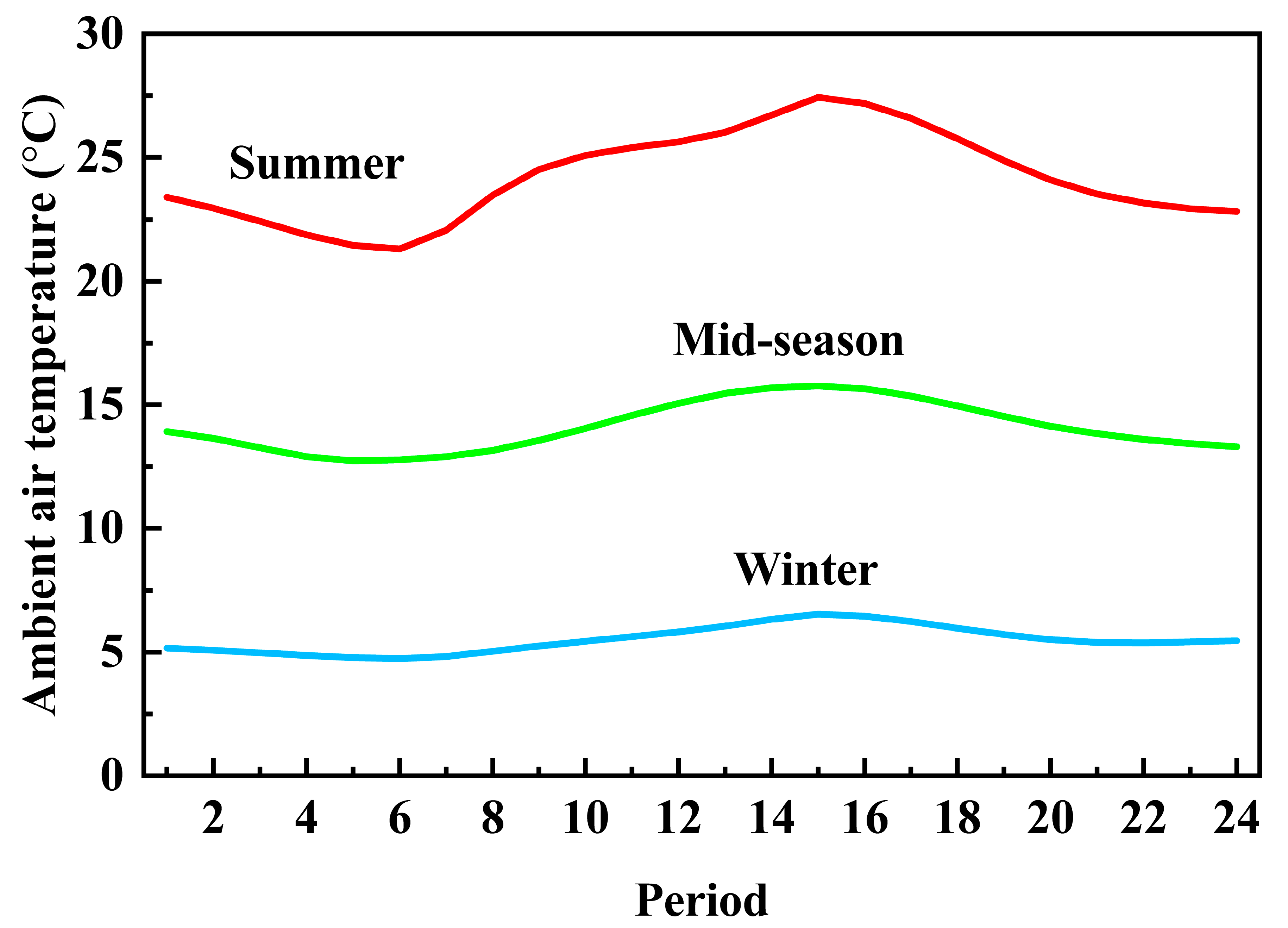
The city is located in the southern part of a warm temperate zone, with an average annual temperature of 14 °C. It has a humid monsoon with slightly maritime climate due to the regulation of the ocean. The four seasons are distinct. Winter is cold and dry, and summer is hot and rainy. Sunlight is sufficient, and rainfall is moderate. The entire year is represented by three typical days, namely, one for each of winter, mid-season, and summer, in accordance with the characteristics of local climate change. The durations of the three typical days are 120, 92, and 153 days, respectively.

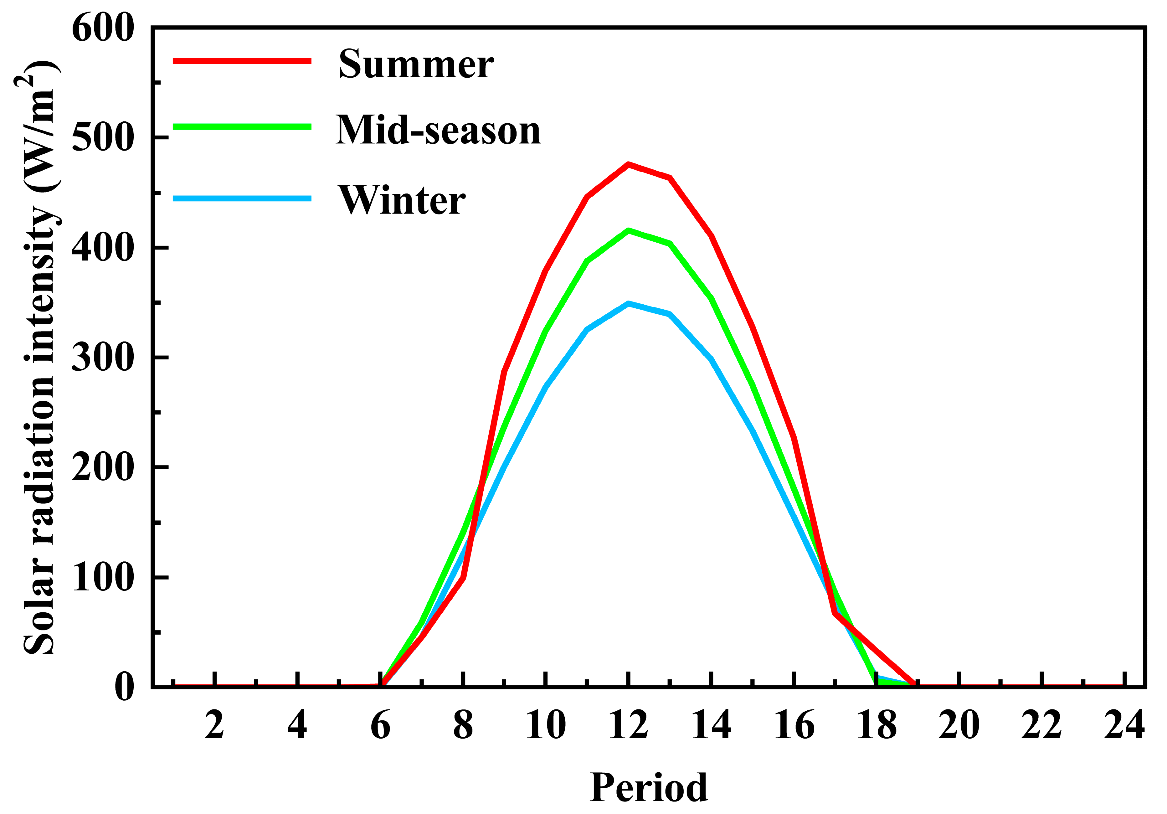
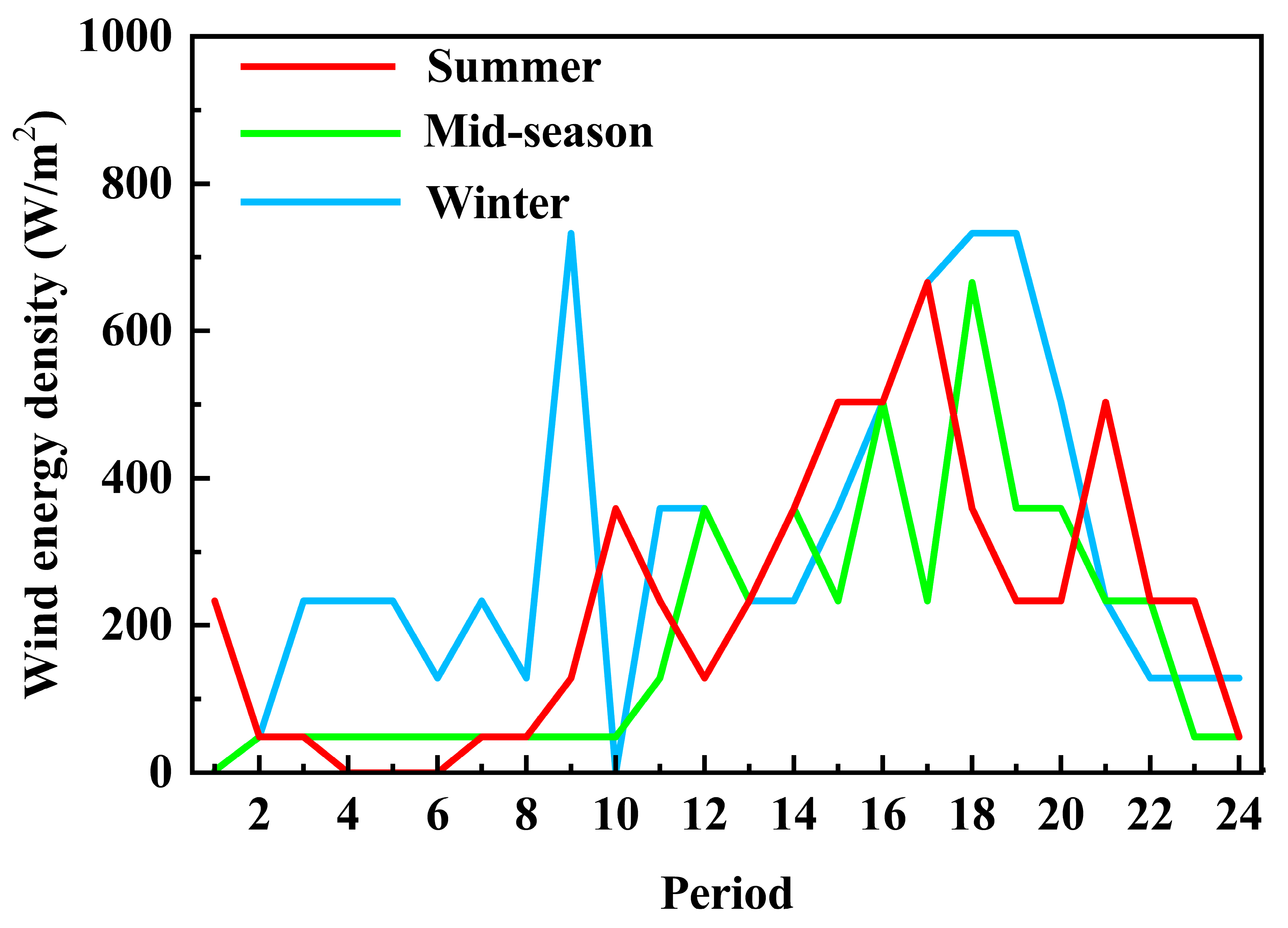
The city has abundant solar energy resources. Annual sunshine time is between 2200 and 3000 h. Total solar radiation for the entire year is between 502 and 586 kJ/cm². Figure 2, Figure 3 and Figure 4 show the hourly values of temperature, solar radiation intensity, and wind energy density for the three typical days.

In this study, each typical day is divided into 24 periods from 01:00 to 24:00, and each period lasts for 1 h. The whole year is divided into 72 periods. This processing method can effectively alleviate the problem of large-scale mathematical programming while ensuring accuracy.

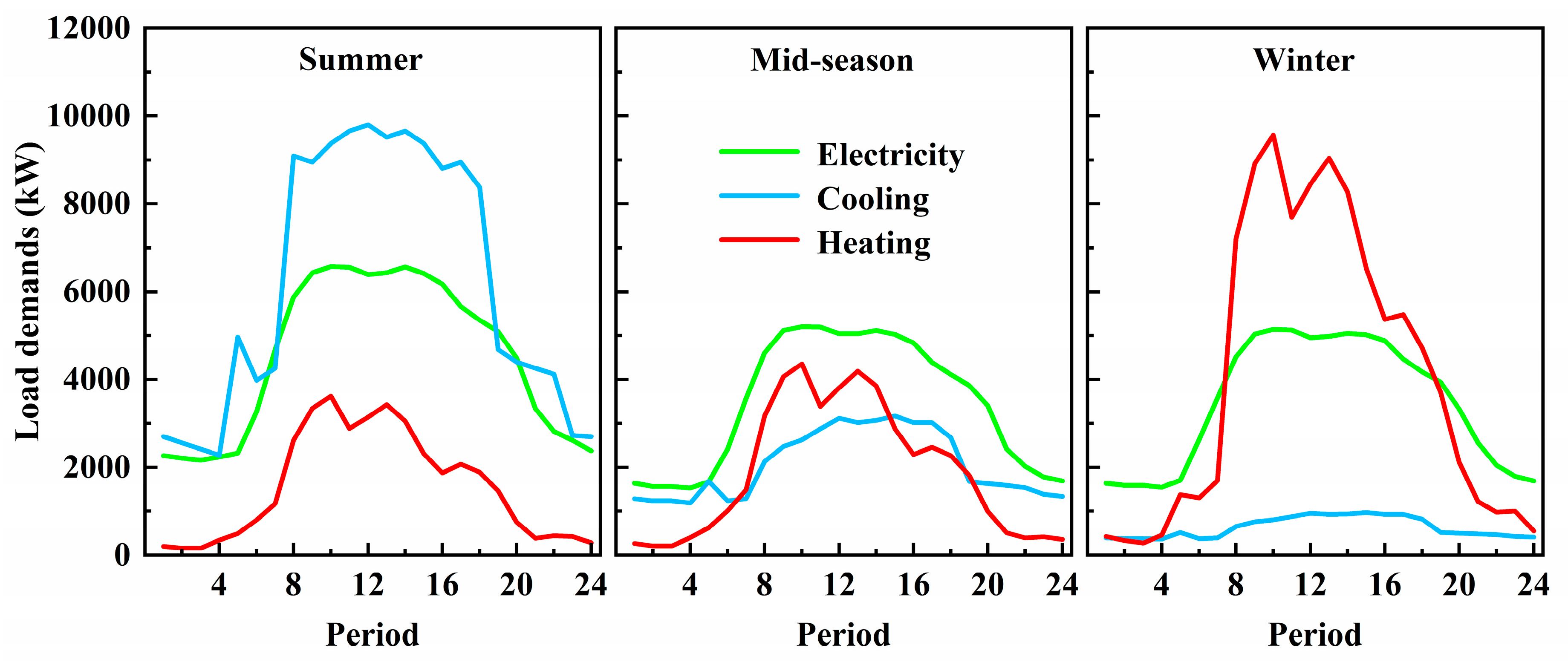
3.2. Load Demands

The hospital selected for the case study has a building area of 294,000 m². The hospital has cooling, heating, and electricity demands throughout the year, with a high daytime load and a relatively low nighttime load. The hourly load demand of the hospital during the three typical days is shown in Figure 5.

3.3. Electricity and Gas Tariffs

The natural gas used in the system is liquefied natural gas with a low calorific value of 41.9 MJ/Nm³ and a price of 0.5505 $/Nm³. The hospital’s electricity is commercial electricity, and the local commercial electricity price is 0.1357 $/kWh.

3.4. DER Equipment Options

The pieces of equipment involved in this system include 4345 and 5200 kW GT; 5200 and 6000 kW GE; 20 kW WT; 28 kW PV; 700 and 1000 kW WB; 700 and 1041 kW GB; 872 and 1454 kW AC; and 1230 and 3520 KW CC, HS and CS. The technical and economic data of these devices are shown in

Table 1. Information of candidate equipment [31,32,33,34].

Equipment Type	Rated Capacity (kW)	Rated Efficiency/COP	Unit Capital and Installation Cost ($/kW)	Unit Fixed O&M Cost ($/kW/year)	Unit Variable O&M Cost ($/kWh)	Load Regulation Range	Lifetime (year)
GT	5200	29.4%	596	0	0.004	0.4–1	15
	4345	28.3%	616	0	0.004	0.38–1	15
GE	5200	40.3%	655	0	0.009	0.4–1	15
	6000	41.2%	635	0	0.009	0.4–1	15
WT	20	35%	1017	0	0.0084	-	25
PV	28	17%	1694	16.7	0.02	-	25
WB	700	78%	130	0	0.0027	0.26–1	15
	1000	78%	130	0	0.0027	0.38–1	15
GB	700	83%	100	0	0.0027	0.48–1	15
	1041	83%	100	0	0.0027	0.26–1	15
HS	-	-	23 $/kWh	-	0.0013	-	20
AC	1454	1.417	172	0	0.001	0.05–1.15	25
	872	1.419	172	0	0.001	0.05–1.15	25
CC	3520	4.73	102	0	0.0015	0.1–1	25
	1230	4.3	102	0	0.0015	0.1–1	25
CS	-	-	23 $/kWh	-	0.0013	-	20

.

4. Setting of Cases

Four cases are designed for comparison and analysis in this work.

Case 1: The system is optimized under deterministic conditions without considering uncertainties.

Case 2: Uncertainties in energy prices (prices of purchased electricity and natural gas) are considered as interval numbers. The radius of the interval is set as 20% of the typical values of energy prices.

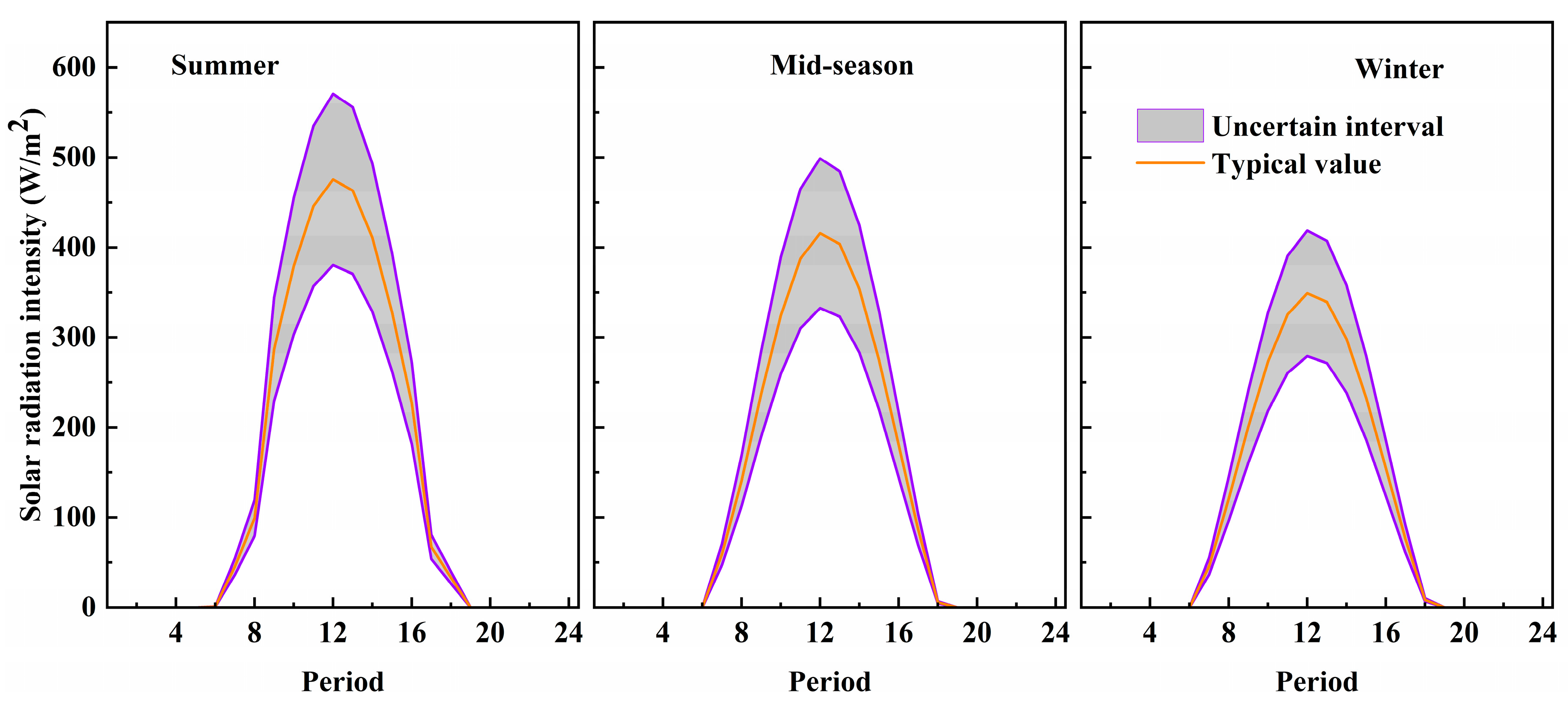
Case 3 (based on Case 2): Uncertainties in energy prices and renewable energy intensity (solar radiation intensity and wind energy density) are considered. The radius of the uncertain interval of renewable energy intensity is set as 20% of the typical values. Figure 6 shows the uncertain interval of solar radiation intensity during the three typical days.

Case 4 (based on Case 3): Uncertainties in energy prices, renewable energy intensity, and load demands (electricity, heating, and cooling demands) are considered. The radius of the uncertain interval of load demands is set as 20% of the typical values.

Probability degrees λ₁ and λ₂ are both set as 0.8, and the weighting coefficient β is also set as 0.8.

The proposed uncertain interval optimization model and the cases were formulated using the optimization software AIMMS 4.29 and solved with the CPLEX 12.6 solver on an Intel^® Pentium^® CPU G620 (2.60 GHZ) with 4 GB RAM.

5. Results and Analysis

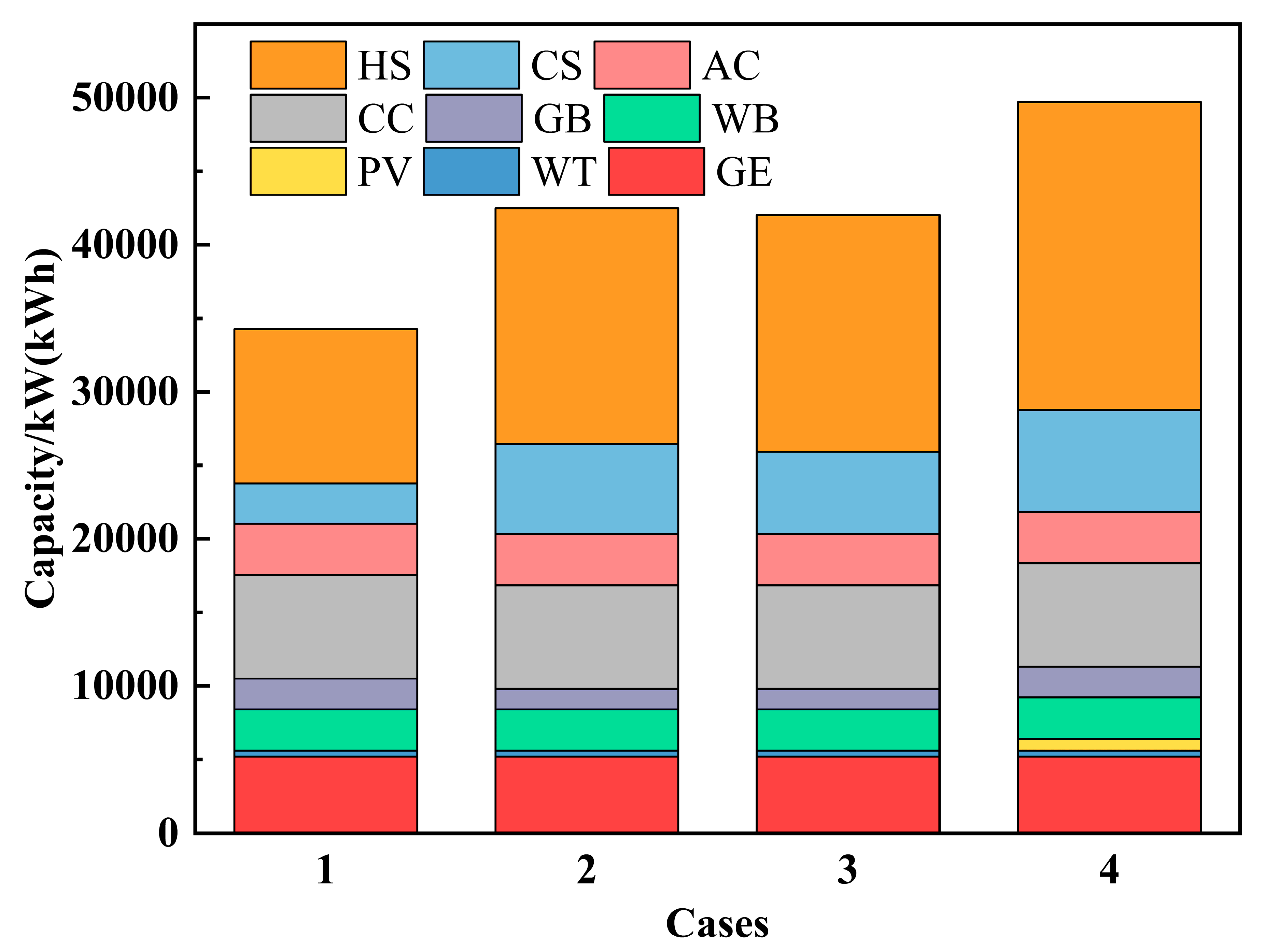
5.1. Optimal System Configuration

After optimization calculation, the optimal system configuration for the four cases were determined as shown in Figure 7. In the deterministic case, the GE and WT are selected as the power generation facility, and exhaust gas from the GE is reused in the AC and WB to generate cold and hot water, respectively. The unmet heating and cooling are provided by the GB and CC. The selected HS and CS can store and release energy during each period to level off the strong constraint of load demands on equipment and to adjust energy flow in the system. The PV system has not been selected because of its high capital cost and low energy efficiency, and the installed number of WT reached its maximum available number.

In Case 2, the selected equipment type is the same as that in Case 1. The installed capacity of the GB decreases from 2100 kW in Case 1 to 1400 kW in Case 2. When the uncertainties in energy prices are considered in this case, the electricity is relatively more expensive than natural gas, and the system relies more on natural gas. The GE operates with a high load rate to generate more electricity and the exhaust gas increases accordingly. Thus, the WB can generate more hot water for the system, and the unmet heating demands that need to be met by the GB reduces, thereby leading to the decrease of installed capacity of the GB. At the same time, the AC generates more cold water, and the cooling met by the CC decreases. To better supply heating and cooling among various time periods, the installed capacity of the HS increases from 10,487 kWh in Case 1 to 16,041 kWh in Case 2, and the installed capacity of the CS increases 2.2 times from 2748 kWh in Case 1 to 6127 kWh in Case 2.

In Case 3, in which uncertainties in renewable energy intensity are added and considered, the optimal system structure remains unchanged, and only the installed capacities of the HS and CS change slightly compared with those in Case 2. In Case 4, in which uncertainties in load demands are also considered, the PV system is installed to generate electricity to meet the increased electricity demands. Compared with that in Case 3, the installed capacity of the GB increases to 2100 kW, which is the same as that in Case 1 and can supplement the increased heating demands. The installed capacity of the HS continues increasing to 20,930 kWh, and the installed capacity of the CS increases to 6929 kWh, improving the ability to regulate energy flow under the larger heating and cooling demands. As can be seen from the Figure 7, the total installed capacity of the equipment in Case 4 is the largest among the four cases.

Overall, uncertainties in energy prices and load demands exert greater impact on system configuration than uncertainties in renewable energy intensity, and uncertainties mostly affect the installation capacities of the GB, HS, and CS, and the selection of PV. Comparing the results of Cases 4 and 1, it can be found that without considering uncertainties, the system configuration may be inappropriate and the installed capacity of equipment may be underestimated.

5.2. Economic Performance

The economic performance of each case is obtained through optimization.

Table 2. Midpoint, radius, lower limit and upper limit of interval of total annual cost in the four cases ($).

	Midpoint	Radius	Lower limit	Upper limit
Case 1	5,816,459	—	—	—
Case 2	5,829,397	907,611	4,921,786	6,737,007
Case 3	5,842,010	910,266	4,931,744	6,752,275
Case 4	6,582,206	1,002,055	5,580,151	7,584,261

provides the total annual cost in the deterministic case, and midpoint, radius, lower limit, and upper limit of the interval of the optimal total annual cost in the uncertain cases.

In Case 1, the total annual cost of the system is a single and deterministic value, because parameters in this case are supposed to be deterministic values. When uncertainties are considered as interval numbers, the total annual cost becomes an interval value, where the midpoint presents the expected value of the cost and the radius indicates the uncertainties of the results because of the uncertainties in the parameters. When the uncertainties in energy prices are considered, in Case 2, the midpoint value of the total annual cost increases by 0.2% compared with the total annual cost in Case 1, mainly due to the increase of the equipment capital investment cost because of the increased installation capacity of storage as described in Section 5.1. The radius of the interval is 15.6% of the midpoint value of the total annual cost, and the interval between the lower and upper limits present the range in which the results may fall. When the uncertainties in renewable energy intensity are added and considered, in Case 3 the midpoint of total annual cost increases by 0.2% compared with that in Case 2, mainly due to the increase of the energy cost, because when there are uncertainties in renewable energy intensity, the system purchases more energy from the market. In Case 4, when the uncertainties in load demands are added and considered, to meet the increased load demands, the system increases the installed capacity of equipment and utilizes more energy resources, leading to the significant increase of the equipment capital investment cost, energy cost, and the total annual cost.

As shown in the table, the midpoint and the radius of the interval of total annual cost increase as the considered uncertainties increase in Case 2 to Case 4, indicating that the uncertainties of the economic results increase and the three types of uncertainties exert a cumulative effect on the optimization results. Uncertainties in load demands have a significant effect on system cost. The comparison of the results of Cases 1 and 4 shows that evaluating the economic performance of the system without considering uncertainties will be over-optimistic.

5.3. Optimal Operation Strategy

The optimal system operation strategy, including optimal dispatch of energy sources and operation status of equipment, was also obtained after optimization. In this section, the optimal operation strategy in Case 4, in which all three uncertainties are considered, is analyzed, and the optimal operation strategy can help decision makers to operate the system appropriately under uncertainties to achieve good system performance.

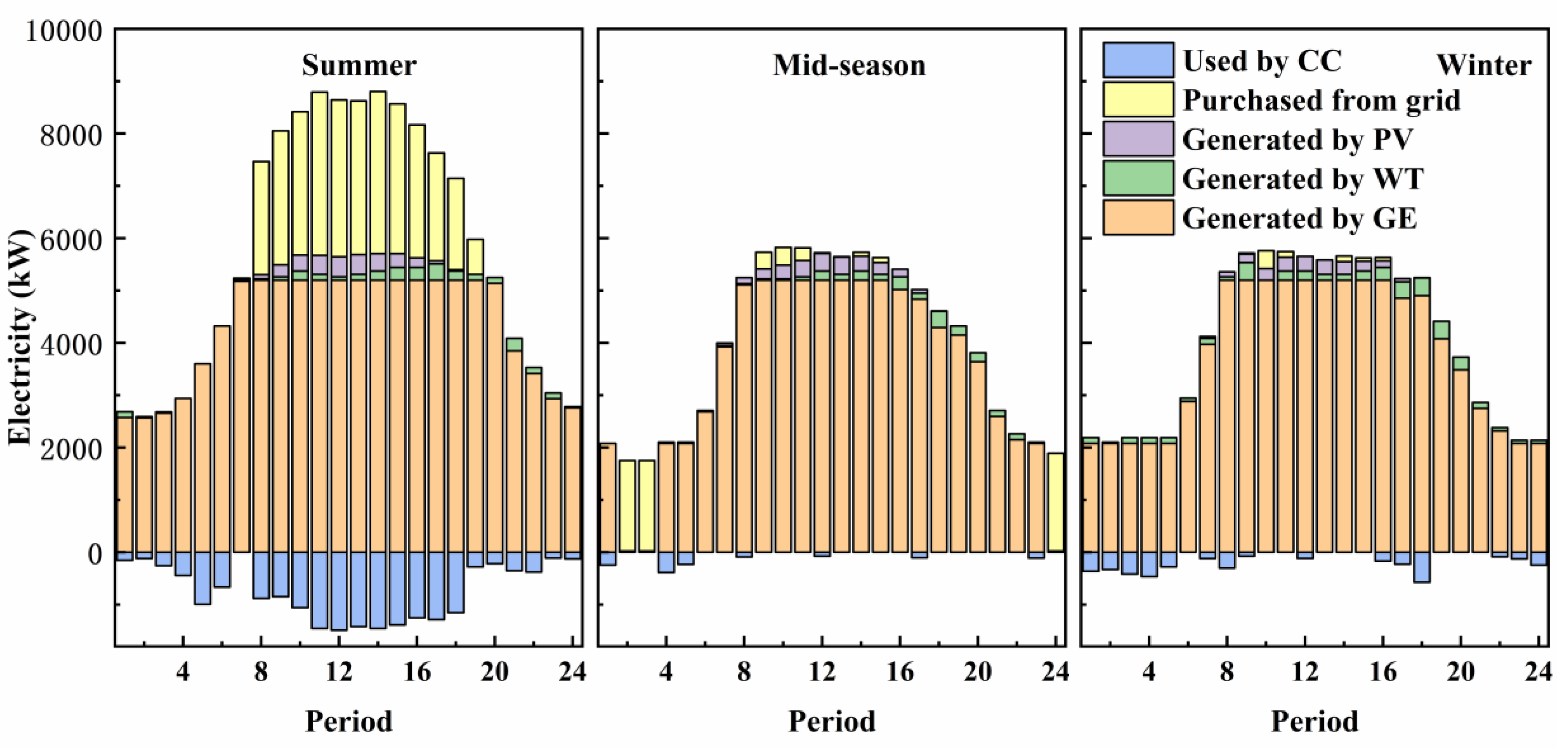
Figure 8 shows the electricity balance in Case 4 during the three typical days. As shown in the figure, the system preferentially uses the GE to provide electricity. When the electricity demands are low, the electricity is mainly provided by the GE. The PV system and WT operate during some periods and provide a small portion of electricity to end users according to the renewable energy intensity. When the electricity demands are beyond the maximum amount of electricity that the GE can generate, electricity is purchased from the grid to meet the extremely high electricity demands. In the 08:00–19:00 periods during summer, a large amount of electricity is purchased from the grid to supplement the unmet demands, and part of the electricity is consumed by the CC to meet the high cooling demands in these periods. In the 02:00–3:00 and 24:00 periods during mid-season, the GE does not operate and the electricity demands of the end users are met mostly by the grid. For the whole year, the electricity generated by the GE and purchased by the grid account for 83.0% and 12.5%, respectively, of the total electricity provided to the end users.

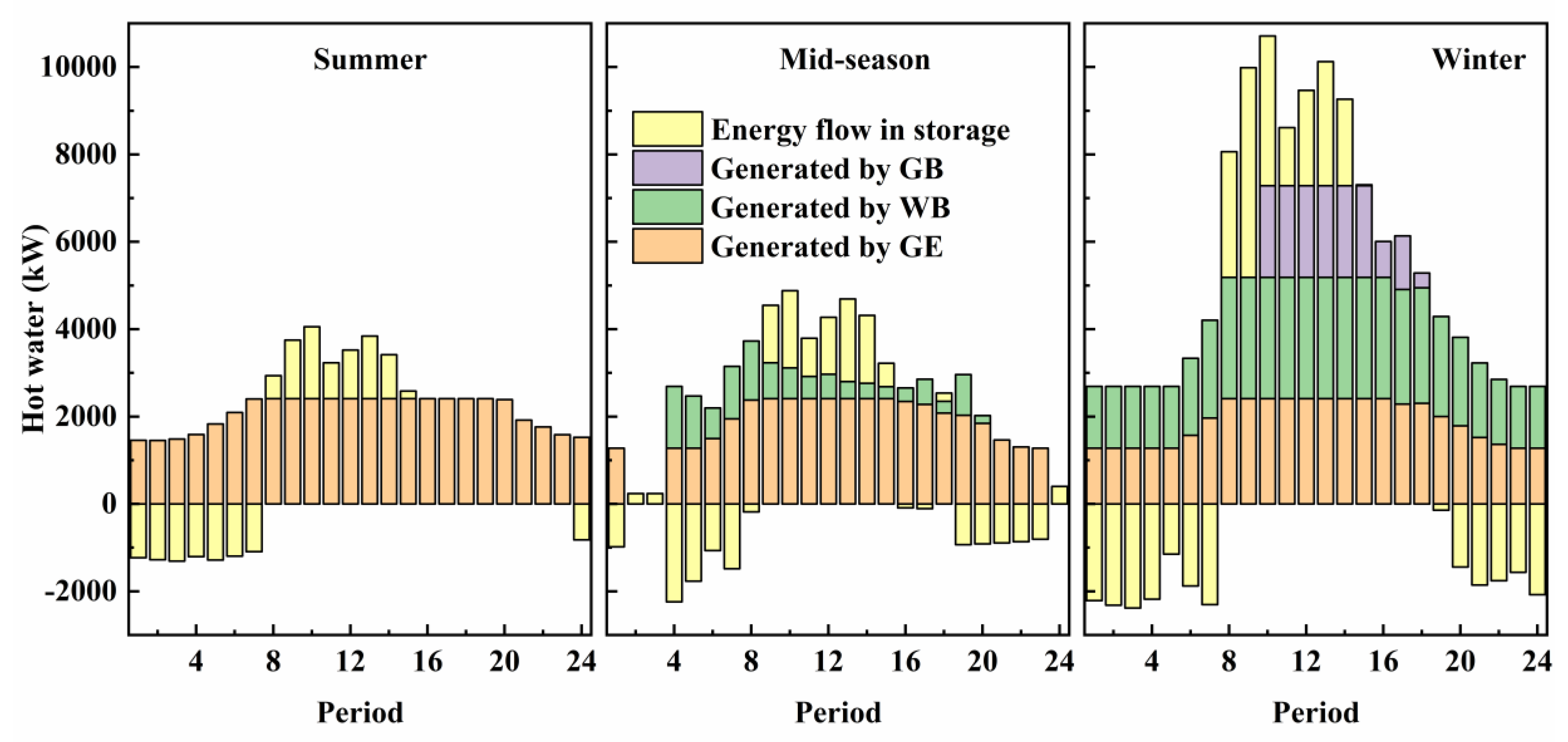
Figure 9 shows the heating balance in Case 4 during the three typical days. During summer, heating demands are met by the GE, and the HS stores heating when the demands are low and releases the stored heating to end users when the demands are high, making the system meet the different heating demands flexibly in periods and achieve good economic performance. During mid-season, the WB also generates hot water in some periods with high heating demands. Notably, the energy required to provide hot water during the two aforementioned typical days is obtained from the waste heat of the GE, without consuming other primary energy sources, indicating the high energy efficiency of this DER system. During winter, the GB operates and supplements the unmet heating demands in the 10:00 to 18:00 periods with high heating demands. The heat released from the HS during winter helps the system meet the extremely high heating demands in 8:00 to 15:00 periods. Without the HS, to meet the extremely high heating demands, the system is required to increase the installed capacity of the GB or WB, leading to an increase in the equipment capital investment cost and reducing system economic performance. For the whole year, the heating generated by the GE and WB account for 65.1% and 28.0%, respectively, of the total heating provided to the end users, and the heating generated by the GB only accounts for 6.9% of the total heating provided to the end users, indicating the high energy efficiency of DER systems.

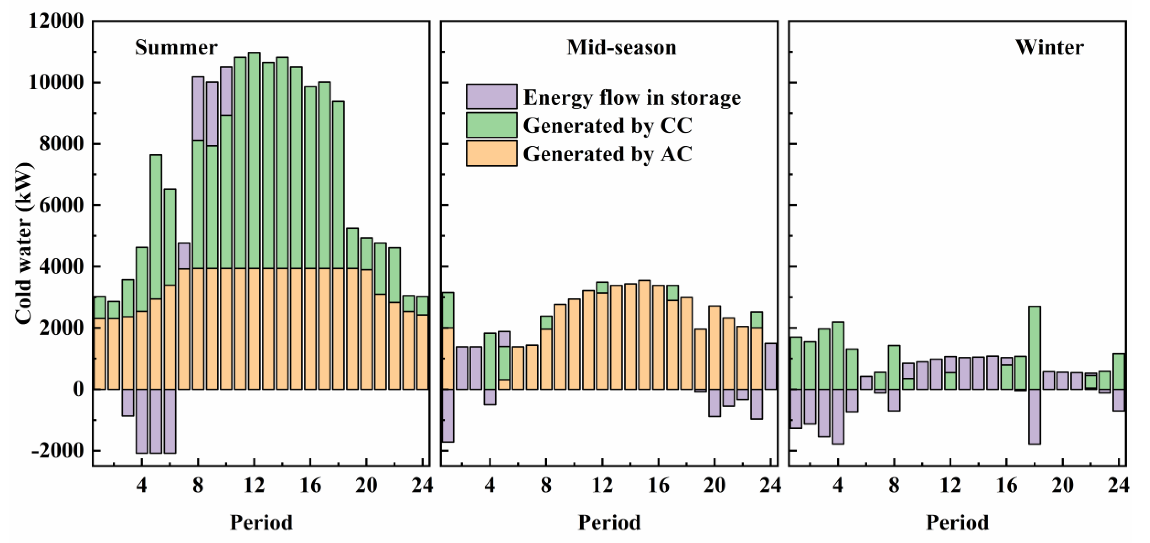
Figure 10 shows the cooling balance in Case 4 during the three typical days. The cooling demands are met by the AC and CC. During summer, the AC reuses the energy in the exhaust gas from the GE and generates cold water to meet the cooling demands, and the unmet cooling demands are supplemented by the AC. The CS stores energy in 03:00 to 06:00 periods and releases the stored energy to end users in 07:00 to 10:00 periods, reducing the strong constraints of cooling demands on the AC and CC and enabling the system to operate flexibly. During mid-season, the cooling demands are mostly met by the AC. In the periods of 02:00–3:00 and 24:00, the AC does not operate because there is no exhaust gas from the GE, and the cooling demands are met by the energy released from the CS. During winter, the cooling demands are largely met by the CC. For the whole year, 52.3% of the total cold water is provided by the AC and 47.7% of the total cold water is provided by the CC.

5.4. Sensitivity Analysis

A sensitivity analysis was conducted to analyze the effects of probability degree and weighting coefficients on system economic performance.

Table 3. Interval of total annual cost with different weighting coefficients and probability degrees ($).

β	λ1	λ2	Midpoint	Radius	Lower Limit	Upper Limit
0.9	0.8	0.8	6,758,731	969,499	5,789,232	7,728,231
0.8	0.8	0.8	6,582,206	1,002,055	5,580,151	7,584,261
0.7	0.8	0.8	6,490,883	1,026,250	5,464,633	7,517,133
0.6	0.8	0.8	6,485,701	1,028,585	5,457,116	7,5142,86
0.8	0.9	0.9	6,745,561	1,057,121	5,688,440	7,802,681
0.8	0.7	0.7	6,283,870	977,995	5,305,875	7,261,865
0.8	0.6	0.6	6,040,841	945,174	5,095,668	6,986,015
0.8	0.5	0.5	5,831,009	907,913	4,923,096	6,738,921

provides the midpoint, radius, lower limit, and upper limit of the interval of total annual cost under different weighting coefficients β and probability degrees λ₁ and λ₂ in Case 4. The table indicates that when β decreases, the midpoint value of the interval of total annual cost also decreases. Meanwhile, the radius of the interval increases. The weighting coefficient β indicates the degree of emphasis on the midpoint value and the radius of the objective interval. The midpoint value represents the average design performance, and the radius represents the sensitivity of the objective value to uncertainties. A small β value ensures the system achieve good expected performance, and a large β value enables the system to achieve better robustness to uncertainties.

When the probability degrees λ₁ and λ₂ decrease, the midpoint and radius of the interval of total annual cost also decreases. The probability degree represents the probability that the constraints can be satisfied. Although a decrease in the probability degree can improve economic performance, the risk that constraints may be violated increases. A trade-off between objective performance and reliability of the solution should be made when choosing the probability degree values.

5.5. Discussion

The optimal system configuration, optimal operation strategy, and the interval of the total annual cost of the system under uncertainties were obtained by applying interval optimization to the optimal design of DER systems. The results show the effects of uncertainties on system configuration and economic performance, and identify the most important uncertainty factors in DER systems. Uncertainties exert a cumulative effect on the system results. When more uncertainties are considered in a system, the system is capable of dealing with more complex real-life situations with uncertainties. However, the deviation of the results of the uncertain case from those of the deterministic case may become larger. In Case 4, the midpoint value of the total annual cost of the system increases by 13.2% compared with total annual cost in Case 1. For the system configuration, the installed capacities of the HS and the CS increase by 2 times and 2.5 times, respectively, compared with those in the deterministic case. It can be easily seen that when operation conditions change, the system configuration obtained under deterministic conditions will be inappropriate and system economy will deteriorate. Designing a DER system with a suitable configuration and operation strategy that can achieve potential benefits in practice requires considering uncertainties as comprehensively as possible and incorporating uncertain optimization methods into the optimization process. The proposed interval optimization model in this work can effectively deal with uncertainties in DER systems and obtain an appropriate solution.

In the work [29], which considers uncertainties in DER systems with SO, the normal, uniform, and Weibull distributions are used to describe various uncertainties. In the current work, the only information needed is the upper and lower limit of uncertain variables, which can be obtained more easily and accurately. Compared to work [29], in the current study the total time periods of the whole year increased to 72, and the optimality gap in the solving process decreased to 0, improving the accuracy of the results. At the same time, the solving time of the model on the same computer dropped from several thousand seconds to several hundred seconds, demonstrating the good calculation performance of interval optimization. Moreover, the interval results of interval optimization can provide decision makers with more information, such as the range in which the possible solution may fall, and the sensitivity of results to uncertainties. In addition, the parameters defined in the formulation and solution processes in interval optimization model in this work, such as probability degree and weighting coefficients, can be selected appropriately to meet various requirements, such as improving the expected performance of the system, increasing robustness to uncertainties, enhancing objective performance, or increasing the reliability of the solution and satisfaction of the constraints in accordance with the attitude of decision makers toward risks and actual conditions.

This research verifies the effectiveness of interval optimization in the optimal design of DER systems under uncertainties. The interval optimization model proposed in this work can be easily extended to more complex energy systems or applied to other real-world problems. By using this method, decision makers cannot only obtain an optimal and robust solution under interval uncertainties, but can also be aware of the uncertainty level of the solution and its sensitivity to uncertainties.

6. Conclusions

An interval optimization-based model for the optimal design of DER systems is proposed in this study, considering uncertainties in energy prices, renewable energy intensity, and load demands, which are presented as interval numbers. On the basis of the order relationship and probability degree of interval numbers, the proposed uncertainty interval optimization model is transformed into a multi-objective deterministic mathematical model, which is further transformed into a single-objective deterministic mathematical model by incorporating a weighting coefficient. The proposed model is applied to a typical hospital in Lianyungang, China, and its effectiveness is verified. Four cases under a deterministic and uncertain environment are designed, and the effects of uncertainties on system optimal configuration and economic performance are analyzed. The optimal operation strategy under uncertainties is also determined. A sensitivity analysis is conducted to analyze the effects of weighting coefficient and probability degree on the interval of total annual cost.

The results show that uncertainties in energy prices and load demands exert significant effects on system configuration and economic performance, primarily affecting the installed capacities of the GB, HS, and CS. The three uncertainties have a cumulative effect on the system optimization results, indicating the importance of comprehensively considering uncertainties. Weighting coefficients and probability degree can be appropriately selected to achieve the designed objective performance in interval optimization. Overall, the application of interval optimization to the optimal design of DER systems can effectively handle various uncertainties and help decision makers obtain a solution that is robust to uncertainties and to become aware of the sensitivity level of the solution to uncertainties.

In the future, other uncertainties in DER systems can be incorporated and considered to obtain a more comprehensive result that is closer to reality. Moreover, a more effective solution method can be developed to address the transformed multi-objective problem in the objective function. Finally, in recent years the importance of considering the rebound effect in energy forecasts has been recognized [35], and the related work in the field of DER systems can be carried out.