Local Market for TSO and DSO Reactive Power Provision Using DSO Grid Resources

Abstract

This paper proposes a near to real-time local market to provide reactive power to the transmission system operator (TSO), using the resources connected to a distribution grid managed by a distribution system operator (DSO). The TSO publishes a requested reactive power profile at the TSO-DSO interface for each time-interval of the next delivery period, so that market agents (managing resources of the distribution grid) can prepare and send their bids accordingly. DSO resources are the first to be mobilized, and the remaining residual reactive power is supplied by the reactive power flexibility offered in the local reactive market. Complex bids (with non-curtailability conditions) are supported to provide flexible ways of bidding fewer flexible assets (such as capacitor banks). An alternating current (AC) optimal power flow (OPF) is used to clear the bids by maximizing the social welfare to supply the TSO required reactive power profile, subject to the DSO grid constraints. A rolling window mechanism allows a continuous dispatching of reactive power, and the possibility of adapting assigned schedules to real time constraints. A simplified TSO-DSO cost assignment of the flexible reactive power used is proposed to share for settlement purposes.

1. Introduction

In traditional power systems, voltage support and reactive power regulation have typically been provided by conventional generators. These generators can be already paid back or still recovering costs mainly through energy markets, and, to a lesser extent, through ancillary services markets. However, under the expected renewable energy sources (RES) integration scenarios, conventional generation units could dramatically decrease in number, due to strict environmental regulations and a lower economic viability (lower prices and lower capacity factors). Under this new framework, new sources of system services must be investigated.

1.1. Related Works

Many approaches can be found for the provision and the corresponding remuneration of reactive power services, grouped under two main alternatives, regulated and market based approaches [1,2,3,4]. Under regulated approaches, reactive power is provided on a mandatory basis: (1) without compensation, at least up to certain limits; (2) compensating a guaranteed reactive power regulation reserve with fixed long-term premiums; (3) compensating the amount effectively dispatched with regulated tariffs; or (4) combining long and short-term regulated compensations to account for investment and operation cost of the resources used. Market based approaches may focus on longer-term agreements for reserve tenders with dispatch prices, or on short-term zonal or nodal dispatching markets.

The costs of providing reactive power depend on the assets, with different responses and regulation capability, but investment costs are in general much larger than operation costs [1]: see for example [5] for static VAR compensators (SVCs) and static synchronous compensators (STACOMs), or [6] for synchronous generators (SGs) and doubly-fed induction generators (DFIGs). Providing reactive power can increase asset losses and decrease other potential revenues. Indeed, SG may need to reduce real power generation to provide the required reactive power, leading to a lost opportunity cost [1,7]. From the cost perspective, as remarked upon in [8], capacitor banks (with lower investments costs but low regulation capacity) should provide steady state reactive power (preferably owned by the TSO), while SG or STATCOM (with larger investments costs but finer reactive power control) should only provide real-time reactive power reserve for dynamic regulation. With this approach, under a generator contingency, the loss of reactive power is lower, and does not increase the reactive power typically needed, due to the overloading of lines by the provision of active power reserves to balance the contingency [8]. However, as remarked upon in [2], expensive reactive power is sometimes needed, because the expensive sources may be more reliable and/or nearer the location that needs the reactive power. At the same time, the cheaper sources may be unable to provide the reactive power to where it is needed, since these types of problems are often local and related with voltage regulation.

While generally accepted that market mechanisms, if appropriate conditions are met, incentivize optimal private investment and efficiency of supply, the question is, for this commodity, if these conditions are really met. Therefore, the question is are the market mechanisms adequate to provide reactive power [3,8,9], or if a regulated cost-of-service remuneration mechanism should be used instead [8]. The fact that reactive power does not “travel” far can lead to local market power, intensified by the fact that a generator withholding reactive power at its bus can congest lines to increase the price for its real power, [3,8]. Other concerns come from the fact that providing reactive power has a frequently very low but volatile variable costs, being large only under contingencies, making pricing harder, [3,10], and possibly leading to price volatilities that could reduce incentives to invest [3]. The above concerns may fit well to traditional power systems where conventional large generators, connected at the transmission grid, and usually belonging to a reduced amount of generation companies, supply most of the reactive power regulation. However, the current energy transition to a renewable mix fostered by more environmental regulations, will probably lead to the progressive closure of CO₂ emitting power plants, and to a large increase of renewable distributed generation (DG), which is rapidly reducing the costs of its investment. This will increase the need for new sources of flexibility to support system services. In addition, new technologies and the behavior of consumers evolving towards more active roles will also increase the number of smaller players, which could have a significant role in market based mechanisms to provide these system services (for example the provision of reactive power), and also reduce the risk of market power. Therefore, if well designed, markets can increase efficiency through market determined prices, and also provide better investment signals for suppliers, with uniform pricing incentivizing bids based on true costs, thus contributing to transparency and fair play [6].

Local markets are a recent approach to integrate these local smaller size distributed resources in market mechanisms to trade energy locally, but also to provide local services to DSO or system services to TSO [11,12]. Local reactive power markets are for example proposed in [13], where the concept of electrical distance is used to decide markets areas, and clearing is performed with a modified Optimal Power Flow (OPF). Only generators provide the service, and their bids consist of four components that represent the costs of producing reactive power, according to [14]. These components are the availability, two types of operation costs and the opportunity cost. Zonal market uniform prices are obtained by minimizing the total payment for the service. In [15], a day-ahead reactive power market is proposed, where both reactive power provision costs and transmission losses are minimized, and the reactive power reserve is provided per detected voltage control areas, similarly to [13]. A multi-objective problem is formulated to minimize the total payments for the reactive power and energy losses, and to maximize system voltage security and reactive power reserves. Finally, [16] proposes a local reactive power market for low level voltage control, where the main providers are electric vehicles.

In [17], reactive power, losses costs and voltages deviations, are all together minimized in a multi-objective minimization problem. A Pareto frontier is proposed, using a non-dominated sorting genetic algorithm II. Reactive power costs come from the reactive power bids offered from the distributed power producers and from the cost of using capacitor banks (being unclear if they are private or DSO resources). Uniform pricing is proposed and computed as the marginal cost of the formulated problem. The problem of recovering investments cost for providing reactive power is not addressed. However, several remarks can be made. First, remunerating the provision of reactive power under a market mechanism can be seen as an improvement, with respect to regulated remuneration mechanisms, so market agents can decide to invest or not for this purpose according to the market prices. Second, the capacity of providing reactive power could need some additional capacity mechanism, as suggested, for example, in [18], but this is not in contradiction with a real time market based on uniform pricing, as occurs with other commodities. In fact, under marginal theory, pricing is not compatible with including fixed costs, since, ideally, price should be equal to the marginal cost of providing the service [19]. For that cases, if the system has evolved in an optimal way, marginal price should allow all units to recover all costs except the marginal unit. If non-supplied service prices are allowed, even the marginal unit could recover all costs in an adapted system. Finally, note that this is not a case of those approaches based on total cost minimization, where variable and fixed costs can be taken into account together in the optimization problem for the medium to long term, as in [20].

Reference [6] proposes a day-ahead distribution grid market, where DG supplies the reactive power. The costs of supplying reactive power are estimated as in the previous references, based on [14]. Clearing is performed based on the cost minimization of providing the service, so the marginal cost is set to the market price. In fact, as in other works, four different market prices are set for the four bids components (availability, two types of operation and opportunity cost). Finally, to cope with DG variability, Monte Carlo scenarios are fed to a multi-objective problem (payments, active power curtailments, line losses and voltage profile index). The problem is solved with a Strength Pareto Evolutionary Strength Pareto Evolutionary Algorithm 2 (ISPEA2). The procurer is the DSO and the coordination TSO-DSO, if any, remains unclear.

Another local reactive power day-ahead market with uniform pricing is proposed in [21] for distribution grids, run by the DSO which is the only procurer. An OPF minimizes the total costs of supplying the service, subject to the grid constraints. The distributed resources are hierarchically organized in microgrids and managed by a central management autonomous controller, which, in turn, controls the lower level microgrids central controllers.

The participation of another type of assets (apart from the conventional generators) is also considered in other works. For example, in [5], losses and reactive provision costs are minimized with special attention to SVC and STATCOM devices. Reference [20] focuses on DG and static compensator costs to provide reactive power in a local combined active and reactive power dispatch based on an OPF. In [6], multiple scenarios are used to reduce the uncertainty of renewable generators. Most approaches are USA markets oriented, where no explicit reactive power bids are made, and clearing is made with an OPF, with the declared technical features and costs of the assets as inputs. In addition, a complex cost description is very often used to represent them in detail (including availability, operation and lost opportunity costs), often considering investments costs for some of the participant assets. Reviews of real approaches to voltage control and reactive power provision and remuneration can be found in [4,22,23].

1.2. Assumptions and Contributions

The present work is part of the Flexibility Hub platform of the Portuguese demonstration of the on-going research project H2020 EU-SysFlex (see funding section). This research focuses on how to ensure an efficient and sufficient level of system services to facilitate very large penetration of renewable energy sources [24]. In this paper, a local reactive power market is proposed to supply, close to real-time, reactive power to the TSO at the TSO-DSO interface by using the resources connected at the distribution grid of the DSO.

The objective is not to address a global reactive power market, whose complexity and power market issues may overcome the benefits. The objective is to propose a local market to allow distributed resources to contribute to the reactive power service, guaranteeing the DSO reactive power responsibility at the TSO-DSO interface, and also provide the additional TSO reactive power needs, guaranteeing that the constraints of the DSO grid are not violated. DSO resources (paid by the users through regulated tariffs) are used first, and the remaining reactive power needed by the TSO is matched with the market bids send by market agents. Some of the main assumptions for the proposed local reactive power market are:

• There is an increasing penetration of distributed energy resources able to provide system services (including DG), and a decrease of conventional plants.
• Market clearing is based on maximizing the social welfare, with uniform pricing to incentivize real marginal costs bidding.
• The agents are responsible from offering their reactive power availability according to their active power program that results from their energy compromises scheduled in energy markets. Note that, as occurs with other interrelated commodities, strategic behavior may lead to modifying other commodity schedules to maximize benefits, but in a technical feasible way (as, for example, occurs in several European markets when units need to make adjustments to their day ahead energy schedule in intraday markets, when secondary reserve capacity is cleared in the secondary reserve market).
• There exists a unique connection point between DSO and TSO grids. However, a methodology has also been developed in the EU-SysFlex to model the impact of multiple connection points, that will be published soon in the Deliverable 6.5 [25].

The main contributions of this paper are:

• A market mechanism to allow distributed market agents to provide reactive power to the DSO and to the TSO, incentivizing the provision of these services from DSO grid resources.
• While most proposals are based on using declared costs as bids, as is usual in USA electricity markets, the current proposal is based on a technical clearing to guarantee grid secure operation, but with a flexible bid format, more aligned with EU markets, leaving more bidding responsibility to the market agents, but also providing them more flexibility.
• A close to real time market for a better reactive power regulation. This allows TSO and market agents to better adapt to variability and uncertainty by continuously adjusting, if needed, their reactive power schedules with buying or selling bids in the overlapping market sessions.
• Complex bids to allow a more flexible operation of the assets, according to their physical constraints (discrete regulation, switching costs, etc.). Clearing is performed by iteratively running a fast multi-period OPF, discarding complex bids when their conditions do not hold, and clearing again with the remaining bids until all the complex conditions of the bids matched hold.
• Both DSO and TSO can use the distributed reactive power resources. Implicit priority is given to the DSO, since bids activation always respects DSO grid constraints. A settlement mechanism to share costs between TSO and DSO is also proposed.

The rest of the paper is structured as follows. Section 2 describes the local reactive market proposed, Section 3 focus on the market clearing, Section 4 describe the main assumptions for the simulated scenarios, Section 5 presents and discusses the results, and Section 6 concludes.

2. Market Description

Figure 1 shows the main agents and system components involved, and the sequence of the main actions that take place during a market session. As can be seen, the TSO publishes the reactive power profile needed (TSO needs) for the next time delivery horizon, so that market agents (flexibility providers) can elaborate and send their bids for each delivery period to supply the TSO needs, or to balance their own position to modify previously assigned schedules. TSO needs are also shared with the DSO, since in a transition phase to a more liberalized system, the DSO can still have its own resources that should be mobilized first to balance the reactive power. The DSO updates the grid topology and the active and reactive power forecasts needed to compute the OPF, and the market is cleared.

To clear the market, the DSO needs the active and reactive power forecasts for all the non-flexible resources of the grid. For the flexible resources participating in the markets, the DSO needs their active power forecasts, their reactive power positions committed in previous market sessions and the bids sent for the current session. For the TSO connection point, the active power is a result of the balance of the DSO grid, and again, the previously reactive power position committed in previous market sessions and the new needs sent for the current session are also needed. It is also notable that, although the current proposal is not considering uncertainty, some more complex clearing could be designed, for example to deal with worst cases. In addition, non-market based real time mechanism, as for other power commodities, could also be available for emergency situations, which should be used to set-up the penalties prices for those not complying with their obligations in the proposed market.

The market is cleared by maximizing the social welfare with network constraints (see Figure 2 and Equations (1) to (10)). When cleared bids have complex conditions not holding, they are iteratively discarded until all complex conditions of the cleared bids hold.

The duration-time of the product delivery is 15 min, and the market is cleared 10 min prior to each delivery. The delivery horizon is set to 7 h (28 time intervals, see Figure 3), so that flexibility providers can use complex bids conditions to, for example, avoiding excessive switching of particular assets (for example for capacitor banks). Indeed, the non-curtailable condition of the bids makes it possible to significantly limit number of switching of assets, and other complex conditions, such as the convexity of the cleared schedule, could also be implemented.

The submission of reactive power bids can take place from the moment the agent is able to estimate its reactive power availability (after a new energy schedule), and until the market session gate closure, ten minutes before the beginning of the delivery horizon (Figure 4).

Bids specify the reactive power offered for each time-period and its price (see for example [20] or [6] for the cost assessment of providing reactive power, as well as Section 4). As referenced, complex conditions can be used to avoid curtailing individual time-periods (for example for discrete steps assets), or to avoid curtailing the whole delivery horizon. Since market sessions are continuously held, after a market session is cleared, only the first time period must be actually delivered (Figure 3). The scheduled reactive power for the following time periods can be adjusted in the following overlapping market sessions, if market liquidity is enough. In this sense, bids and reactive power assignments must be understood as incremental with respect to the current reactive power schedule resulting from all overlapping previous market sessions.

3. Market Clearing

Each market session is cleared by maximizing the social welfare (maximizing the utility of the cleared buying bids and minimizing the cost of the cleared selling bids) for the whole amount T of time periods t of the delivery horizon and for total number F of flexibility resources f (generators or capacitor banks), according to Equation (1):

$$Max{\displaystyle \sum _t^T}{\displaystyle \sum _f^F}\left(\begin{array}{l}-{\displaystyle \sum _i^{N{B}_{Cap}{}_{f,t}}}p{b}_{i,f,t}^{cap}\times \Delta Q_{i,f,t}^{B_{cap}}-{\displaystyle \sum _i^{N{S}_{cap}{}_{f,t}}}p{s}_{i,f,t}^{cap}\times \Delta Q_{i,f,t}^{S_{cap}}\\ +{\displaystyle \sum _i^{N{B}_{ind}{}_{f,t}}}p{b}_{i,f,t}^{ind}\times \Delta Q_{i,f,t}^{B_{ind}}+{\displaystyle \sum _i^{N{S}_{ind}{}_{f,t}}}p{s}_{i,f,t}^{ind}\times \Delta Q_{i,f,t}^{S_{ind}}\end{array}\right)$$

(1)

where “cap” stands for capacitive and “ind” for inductive, $p{b}_{i,f,t}$ and $p{s}_{i,f,t}$ are the buying and selling prices of the corresponding bid i of a flexible resource f for time period t, and $\Delta Q_{i,f,t}^{B_{cap}}<0$, $\Delta Q_{i,f,t}^{B_{ind}}>0$ and $\Delta Q_{i,f,t}^{S_{cap}}>0,$ $\Delta Q_{i,f,t}^{S_{ind}}<0$ are the decision variables corresponding to the cleared buying and selling quantities, respectively. $N{B}_{Cap}{}_{f,t},N{B}_{ind}{}_{f,}$ and $N{S}_{cap}{}_{f,},$ $N{S}_{ind}{}_{f,}$ are, respectively, the total number of offers to buy (capacitive and inductive) and to sell (capacitive and inductive) of a flexible resource f at time period t. It is also notable that, after clearing the market, $\Delta Q_{i,f,t}^{B_{cap/ind}}$ and $\Delta Q_{i,f,t}^{S_{cap/ind}}$ are incremental assignments, with respect to the current reactive power position of the flexible resource f for the time period t (as a result of previous overlapping market sessions). In addition, the cleared quantities are limited by the maximum quantities offered and by the typical optimal power flow constraints [26] described below. The optimization algorithm used is based on the primal-dual interior point method as explained in [27]. This method was chosen because of its robustness when applied to non-convex problems, such as OPF [28]. Note that other optimization algorithms, such as a convex relaxation of OPF [29] or hybrid PSO [30] could also have been used.

$$P_{n,t}^G-P_{n,t}^D-P_{n,t}=0,\forall n\in N,\forall t\in T$$

(2)

$$\left(\Delta Q_{n,f,t}^{ind}+\Delta Q_{n,f,t}^{cap}+Q_{n,t}^G\right)+\left(\Delta Q_{n,f,t}^{cond}+Q_{n,t}^{cond}\right)-\left(Q_{n,t}^D\right)-Q_{n,t}=0,\forall n\in N,\forall f\in F\mathrm{and}\mathrm{connected}\mathrm{at}n,\forall t\in T$$

(3)

$$V_{n,t\left(min\right)}\le \left|V_{n,t}\right|\le V_{n,t\left(max\right)},\forall n\in N,\forall t\in T$$

(4)

$${\varphi }_{t,ref}=0,\forall t\in T$$

(5)

$$Q_{n,t}^{cond}\in \{Q_{n,t}^{cond}\},\forall n\in N_{cb},\forall t\in T$$

(6)

$$ta{p}_{l,j,t}\in \{ta{p}_{l,j,t}\},\forall t\in N_{OLTC}$$

(7)

$${\left|S_{b,t}\right|}^2\le {(S_b^{max})}^2,\forall b\in Br,\forall t\in T$$

(8)

where for time each time period t:

$$P_{n,t}=\left|V_{n,t}\right|{\displaystyle \sum }_{k\in B{r}_n}^{}\left[\left|V_{k,t}\right|\left(G_k\times cos{\theta }_{k,t}+B_k\times sin{\theta }_{k,t}\right)p\right]$$

(9)

$$Q_{n,t}=\left|V_{n,t}\right|{\displaystyle \sum }_{k\in B{r}_n}^{}\left[\left|V_{k,t}\right|\left(G_k\times sin{\theta }_{k,t}-B_k\times cos{\theta }_{k,t}\right)\right]$$

(10)

Equation (2) is the active power balance where $P_{n,t}^G,P_{n,t}^D$ and $P_{n,t}$ are the sum of active power from all generators, loads and lines at node n for time period t. N is the total number of nodes.

Equation (3) is the reactive power balance at node n. It is computed from the initial reactive power operation point (by summing the reactive power of the generators at node n, $Q_{n,t}^G$, the reactive power of the capacitor banks at node n, $Q_{n,t}^{cond}$, the reactive power of the loads at node n, $Q_{n,t}^D$, and the total lines’ reactive contribution at node n, $Q_{n,t}$) by adding $\Delta Q_{n,f,t}^{cap}$ and $\Delta Q_{n,f,t}^{ind}$, the total cleared capacitive and inductive reactive power flexibilities, as well as $\Delta Q_{n,f,t}^{cond}$, the total cleared reactive power flexibility provided by the capacitor banks.

Equation (4) limits the voltage magnitude $V_{n,t}$ to its maximum and minimum values, $V_{n,t\left(max\right)}$ and $V_{n,t\left(min\right)}$, respectively, and Equation (5) sets the voltage angle at the reference bus.

Equations (6) and (7) model the discrete steps positions of the capacitor banks, $Q_{n,t}^{cond},$ and of the on-load tap changers (OLTC), $ta{p}_{l,j,t}$, respectively ($N_{cb}$ and $N_{OLTC}$ being the number of capacitor banks and OLTCs, respectively).

Equation (8) limits the direct and inverse branch flows $S_{b,t}$ to their thermal limit $S_b^{max}$, Br being the set of all grid branches.

Finally, Equations (9) and (10) are the active and reactive power, $P_{n,t}$ and $Q_{n,t}$, respectively, provided at node n by the branches k connected to node n (set $B{r}_n$) for each time period t. In these equations, $V_{k,t}$ is the voltage at the other node the branch k is connected to, G_k and B_k are the real and imaginary parts of the admittance of line k, and ${\theta }_{k,t}$ is the difference in voltage angle (at time t), between the two nodes the line is connected to.

Note that complex condition checking is not reflected in Equations (1) to (10), since this is based on checking, after the clearing process of Equations (1) to (10), if the complex conditions of the bids cleared hold. Otherwise, these bids are discarded, and the market is cleared again with the remaining bids. This is therefore reflected only Figure 2, in the loop used to check the complex conditions of the bids.

It is also notable that, since, with this approach, two different products are in fact being traded, two different market prices must be considered, one for the capacitive reactive power, corresponding to the most expensive cleared selling bid of capacitive reactive power, and one for the inductive reactive power, corresponding to the most expensive cleared selling bid of inductive reactive power. Finally, DSO resources, if any, are cleared first by considering them with null price to sell, and maximum price to buy, so that only the remaining reactive power demand needs to be supplied by the market players.

4. Study Cases

According to [20], Figure 5 shows the costs incurred by solar photovoltaic (PV) and wind farms to provide both inductive and capacitive reactive power, both related to the losses caused by the extra current to provide reactive power.

As can be seen, total costs for PV farms depend on the active power operating point (basically due to the inverters maximum current limitation), unlike wind farms [20]. Since, under marginal theory markets, bid prices are based on variable (marginal) costs, for simplicity reference costs have been selected for both types of assets, set to 5 EUR/MVArh for the PV assets and to 3.5 EUR/MVArh for the wind generation assets. Price bids have then been obtained with small deviations from this reference costs, as shown in Figure 6, using σ = 0.2.

Indeed, according to standard marginal theory, market players may be willing to provide (sell) inductive or capacitive power if price is larger than the marginal costs of providing it (selling bid price larger than the reference cost in this simplified case example), but could also be willing to reduce the reactive power scheduled in a previous market session (buy), if the price is lower than the marginal costs of providing the service (buying bid price lower than the reference cost). It is also notable that, for simplicity, all the available reactive power is being offered in a unique block in this example. However, market agents could, in general, break down this block into smaller ones to offer a stepwise quantity-price curve, to better represent non-constant marginal costs, as happens in many other power markets in Europe.

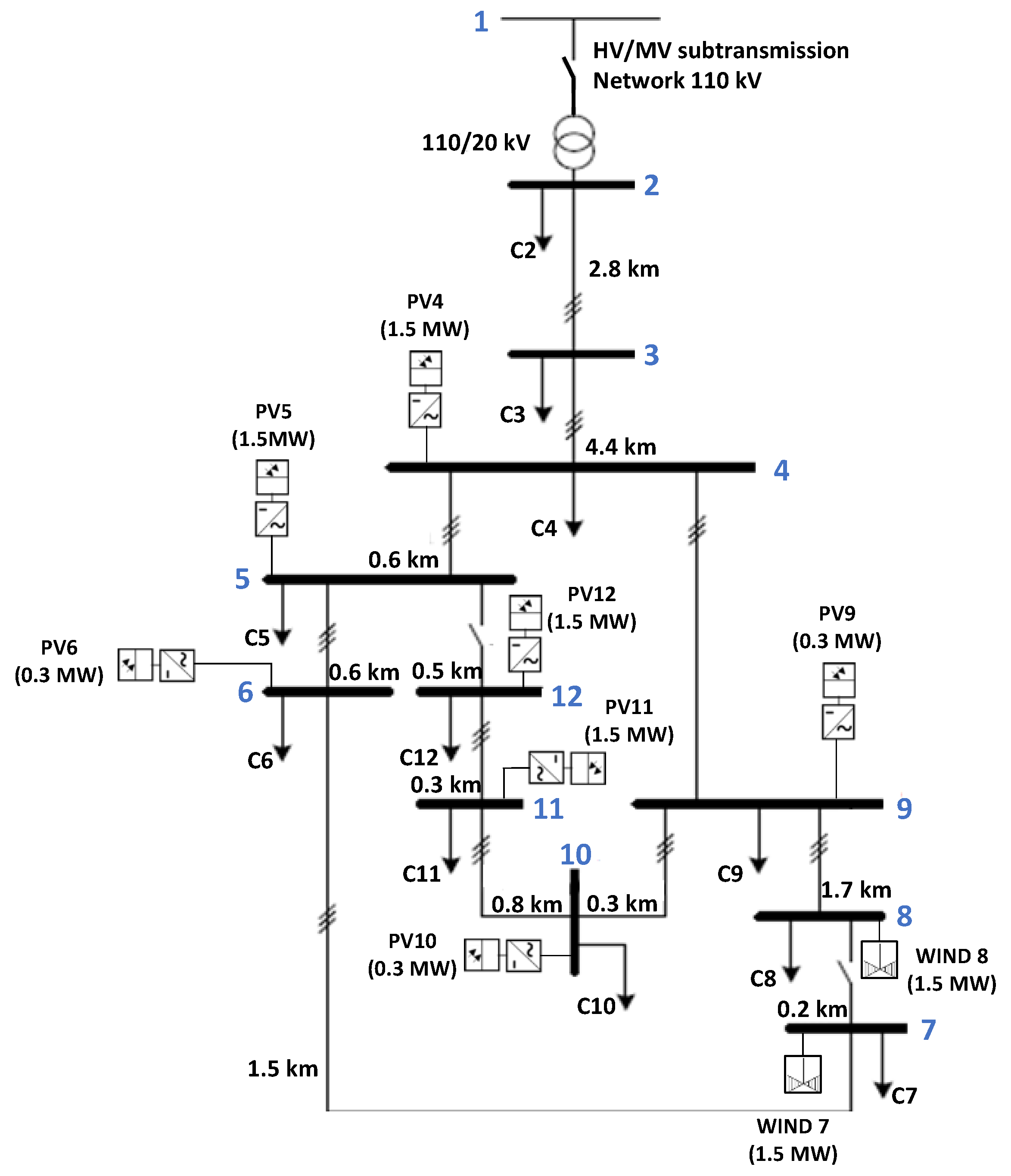
Figure 7 represents the grid used for the simulated case examples, based on a simplification of the one proposed in [31], and

Table 1. P and Q operating point of consumers and generators.

Consumers	P [MW]	Q [MVAr]	Generators	P [MW]	Q [MVAr]	∆Q [MVAr]	Price [EUR/MVAr]
C2	−6.4375	−0.9081	PV4	1.0000	0.0000	1.1200	5.0000
C3	0.0000	0.0000	PV5	1.0000	0.0000	0.0000	0.0000
C4	−0.1235	−0.03000	PV6	0.0200	0.0000	0.0000	0.0000
C5	−0.1929	−0.04690	PV9	0.0150	0.0000	0.0000	0.0000
C6	−0.3251	−0.07900	PV10	0.0300	0.0000	0.0000	0.0000
C7	−0.2449	−0.05950	PV11	1.0000	0.0000	0.0000	0.0000
C8	0.0000	0.0000	PV12	1.0000	0.0000	1.1200	5.0000
C9	−0.2622	−0.06380	WIND7	0.3000	0.0000	1.5000	3.5000
C10	0.0000	0.0000	WIND8	0.3000	0.0000	1.5000	3.5000
C11	−0.2124	−0.05160
C12	−0.1473	−0.03580

shows the consumers (left side) and generators (right side) connected to the grid, and their operation point in terms of active and reactive power. The numbers in the acronyms refer to the node in Figure 7 to which they are connected. For the generation assets, their installed capacity, and their reactive power flexibility and reference cost used are also in the table. For simplicity, only four resources have been selected to offer reactive power flexibility. Their first reactive power operating point can be considered as the result of using their reactive power bids to compensate the consumers reactive power when the TSO is not demanding, whose cost could be recovered by the DSO through distributions tariffs. Note, however, that there could also be a scenario where consumers could also participate in the local reactive power market in the same way as the generators do.

5. Results

Two scenarios have been tested, considering, for simplicity, a sequence of market sessions with only one time period and no complex bids. The first scenario corresponds to the TSO demanding increasing inductive reactive power (modelled with a capacitive reactive power injection to the DSO grid that must be compensated with inductive reactive power from the flexible resources). The second scenario corresponds to increasing TSO capacitive reactive power needs (modeled with an inductive reactive power injection to the DSO grid). For illustrative purposes, starting from 0 TSO needs in both cases (which clears the reactive power needed by the DSO to compensate its grid reactive power), TSO needs are incremented with −1 MVAr steps until −5 MVAr in the first scenario, and incremented with 0.1 MVAr steps until 0.4 MVAr in the second scenario.

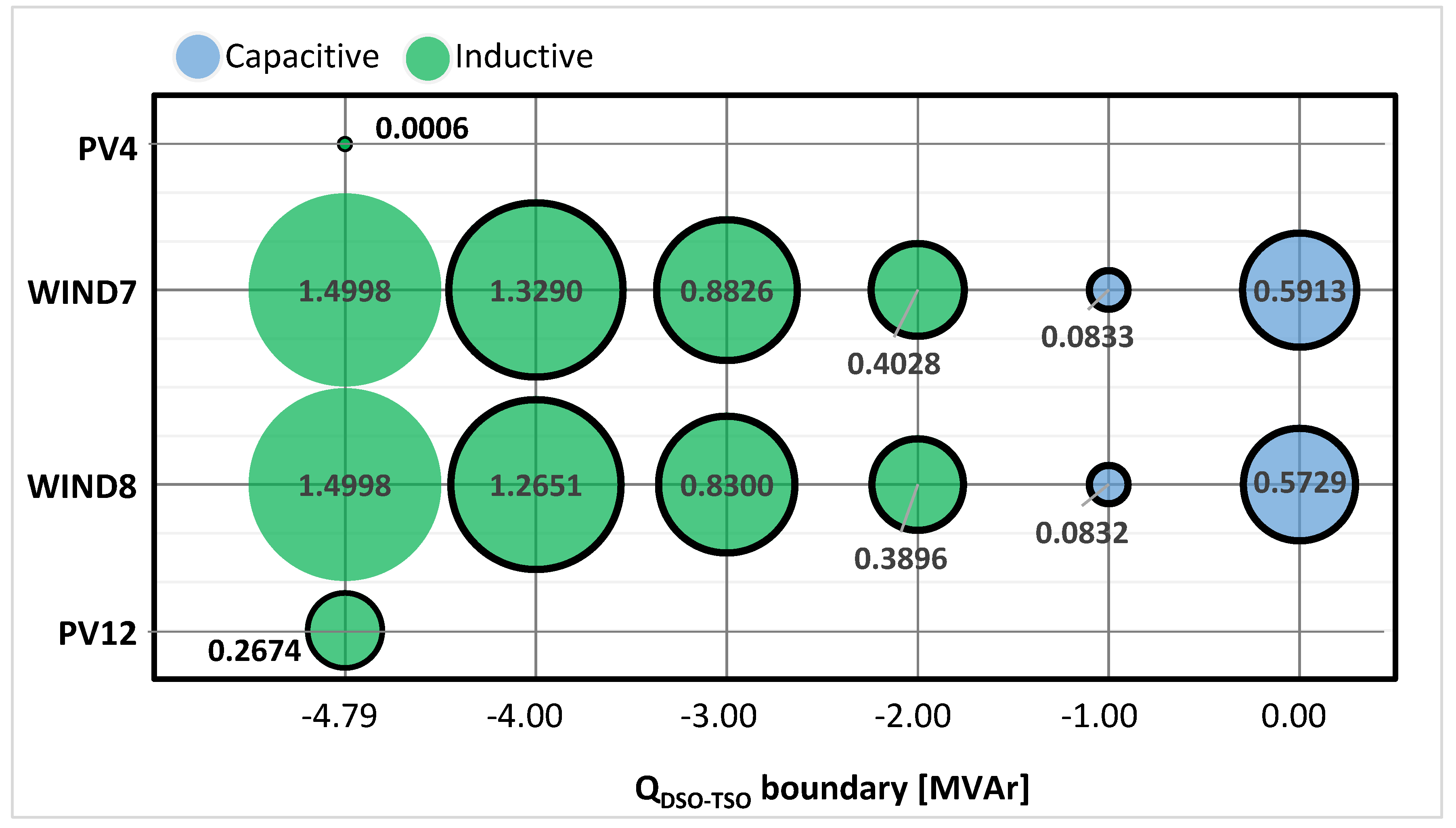
Figure 8 shows the reactive power provided by each of the flexible providers after clearing the market, for increasing TSO inductive needs (blue circles correspond to capacitive reactive power, green circles to inductive, and a black border indicates those resources that are setting the market price).

Initially, when the TSO is not demanding reactive power, the cheapest resources (WIND7 and WIND8 with same price) provide the capacitive reactive power needed by the DSO to compensate the loads inductive reactive power of its grid, setting the market price to 3.7 EUR/MVAr. Note that, since WIND7 and WIND8 are located at different buses, their contribution is not symmetric, with WIND7 being the resource that provides more capacitive reactive power, since its contribution is subject to less reactive power losses (and has therefore a larger positive impact on the social welfare).

When the TSO increases its inductive needs, the same providers can buy the amount of reactive power already cleared and now partially provided by the TSO. Since sells have a price larger than the reference cost, and purchases lower, all operations entail benefits for the providers. When the TSO needs reach an inductive reactive power between −1 and −2 MVAr, all the reactive power of the loads is compensated, and additional inductive reactive power is needed and provided from the same cheaper providers, with same market price. When a TSO value between 4 and 5 MVAr is reached, more inductive reactive power is needed, and more expensive providers are then cleared (PV4 and PV12), increasing the market price to 5.2 EUR/MVAr. 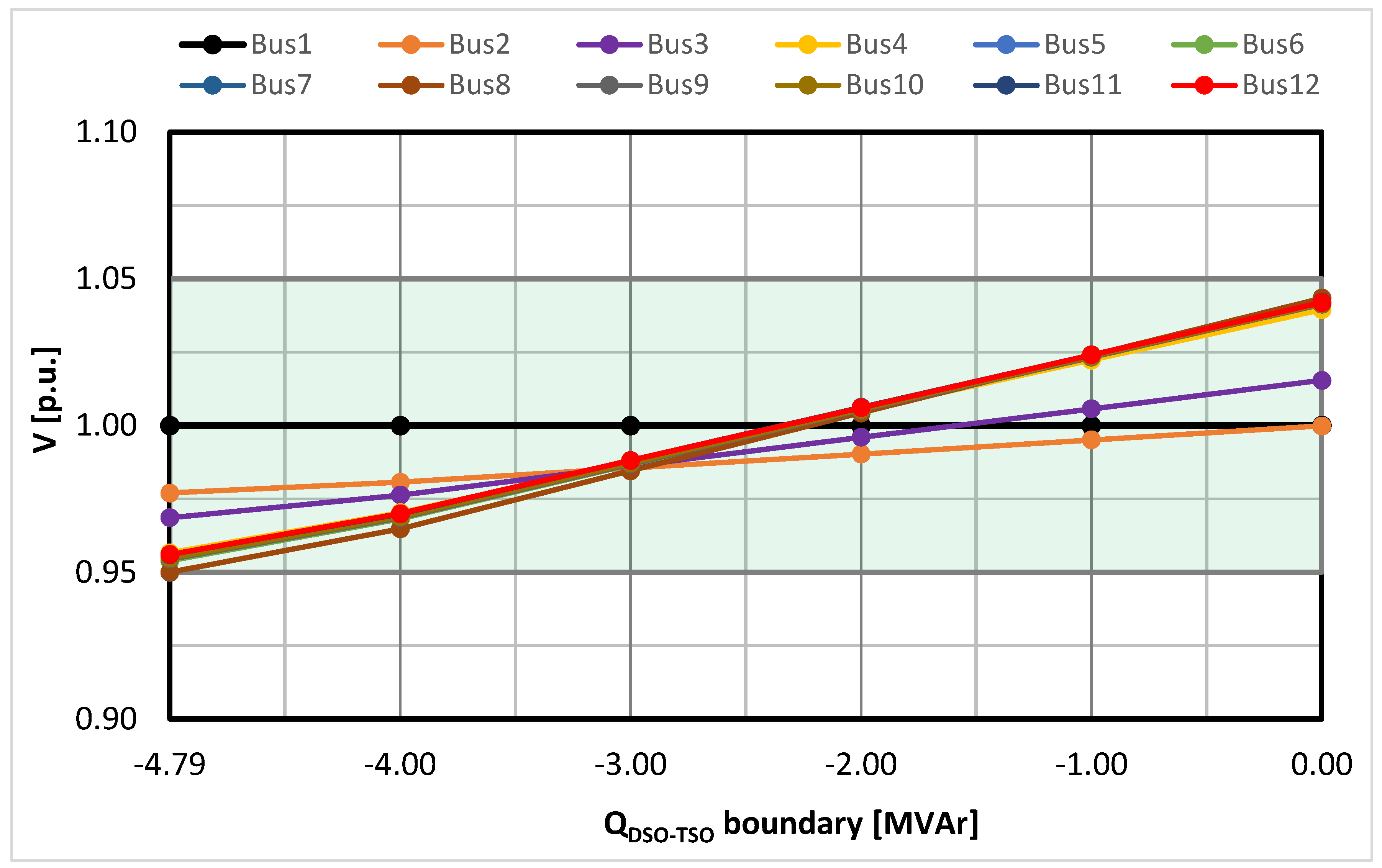Figure 9 shows the buses’ voltage in the grid for each TSO reactive inductive needs.

The capacitive reactive power injection decreases bus voltages with bus 10 reaching its minimum limit near TSO needs of −5 MVAr (note that bus 1 voltage is modeled as constant and equal to 1). This is consistent with Figure 10, which shows how lines flows increase (increasing voltage drops) when the TSO demands more inductive reactive power. In fact, when bus 10 reaches the 0.95 pu voltage, the reactive power provided to the TSO is limited by this voltage constraint, and TSO does not reach all the demanded value (by around −0.21 MVAr), although there is still reactive power flexibility unused.

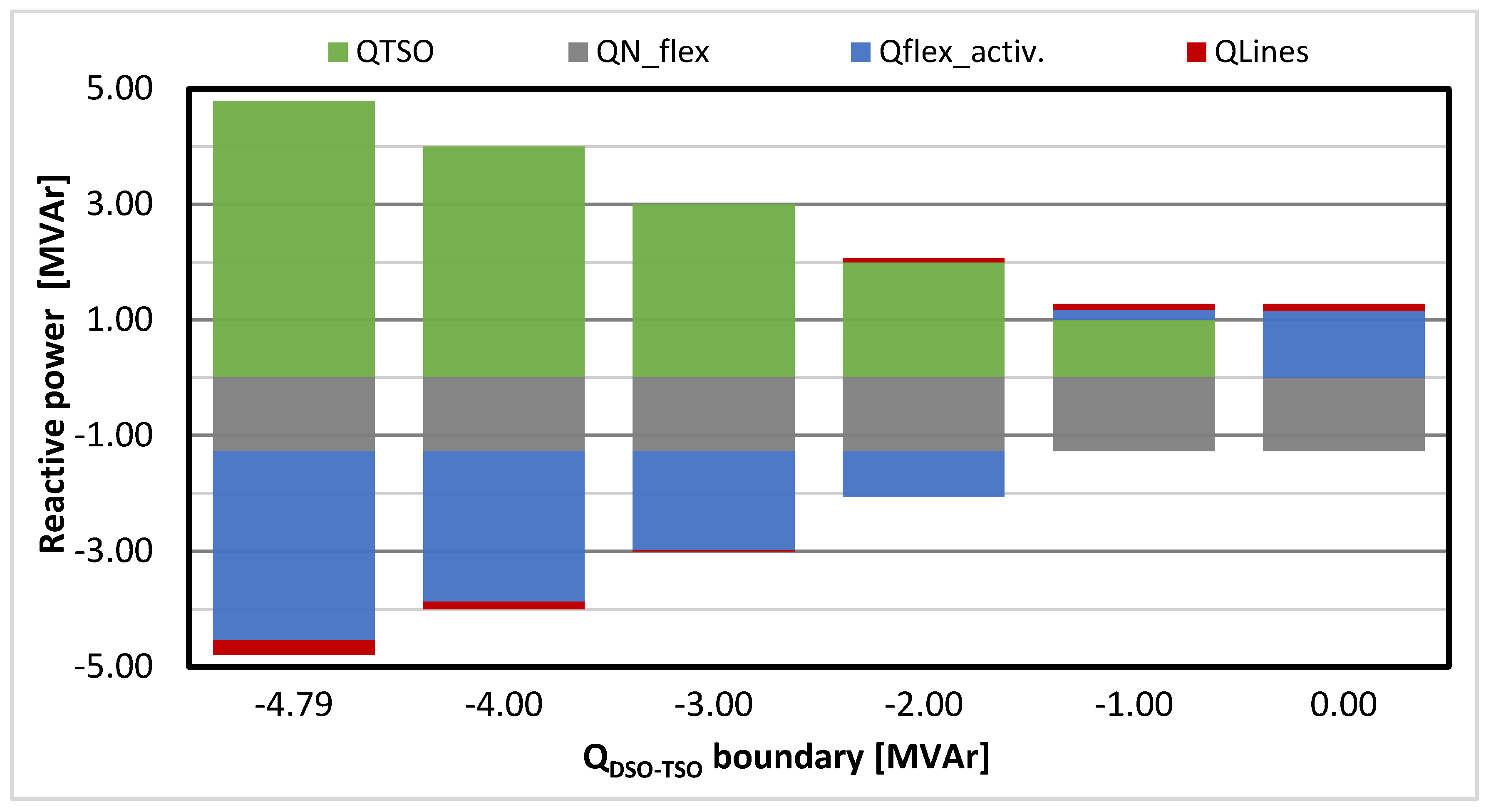
Figure 11 shows the total reactive power injection of the TSO, non-flexible resources, flexible resources and lines contribution, as described in Equation (3). As the TSO inductive needs increase, so does the inductive flexibility provided by the flexible resources, and it can also be seen how the lines’ reactive power contribution switches from capacitive to inductive injection.

The use of the activated flexibility $\Delta Q_{flex.activ.}$ of a particular delivery time of a market session is explained by Equation (11), where $\Delta Q_{tso}$ is the increment of the reactive power consumed by the TSO at the DSO-TSO boundary and $\Delta Q_{dso}$ is the increment of the reactive power the DSO needs to equilibrate its reactive power grid (note that inductive TSO needs correspond to a capacitive consumption, which with the consumer criteria of Equation (11) becomes negative). This DSO reactive power, $\Delta Q_{dso}$, see Equation (12), consists of $\Delta Q_{N\_flex}$, the reactive power needed to compensate the non-flexible resources forecast variation (that could be updated at each market session), and $\Delta Q_{lines}$, needed to compensate the variation of the lines’ reactive power (which may change with $\Delta Q_{tso}$ and $\Delta Q_{dso}$).

$$\Delta Q_{flex.activ.}=\Delta Q_{tso}+\Delta Q_{dso}$$

(11)

$$\Delta Q_{dso}=\Delta Q_{N\_flex}+\Delta Q_{lines}$$

(12)

Table 2. Reactive power balance for increasing TSO inductive needs at each market session.

	Session 1	Session 2	Session 3	Session 4	Session 5	Session 6
∆QTSO [MVAr]	0.0000	−1.0000	−1.0000	−1.0000	−1.0000	−0.7897
∆QN_flex MVAr]	1.2747	0.0000	0.0000	0.0000	0.0000	0.0000
∆QLines [MVAr]	−0.1105	0.0023	0.0411	0.07980	0.1185	0.1162
∆Qflex_activ. [MVAr]	1.1642	−0.9977	−0.9589	−0.9202	−0.8815	−0.6735

presents the reactive power contribution of each the concepts involved in Equations (11) and (12) for the first scenario analyzed. At the initial null reactive power of the TSO, the reactive power flexibility is only used to compensate the DSO grid, providing capacitive reactive power. As the TSO inductive needs increase (see also Figure 8), assuming that the non-flexible reactive power remains constant, so does the inductive flexibility provided by the flexible resources.

It is interesting to note how the reactive power of the lines can, depending on their loading [32], reduce or increase the net DSO reactive power needs. For the scenario in Table 2, lines reactive power decreases the total amount of flexible reactive power needed by the DSO to equilibrate its grid, therefore reducing its costs.

For a particular delivery time of a market session, settlement is obtained by computing the net collection rights of the flexibility providers, $E{R}_{Q_{Flex}}$, Equation (13), and the net obligations to pay of the flexibility users, that is $E{O}_{Q_{TSO}}$ for the TSO, Equation (14), and $E{O}_{Q_{DSO}}$ for the DSO, by isolating in Equation (15). Note that, even if the TSO is an inelastic player (that buys at maximum price and sells at minimum price), its net payment obligation is the opposite of the collection right of a flexibility provider (due to the buyer criteria selected for the TSO).

$$\begin{array}{cc}\hfill E{R}_{Q_{Flex}}& =\left(\Delta Q_{Flex}^{S_{cap}}·{\lambda }_{cap}-\Delta Q_{Flex}^{S_{ind}}·{\lambda }_{ind}\right)\hfill \\ \hfill +& \left(\Delta Q_{Flex}^{B_{cap}}·{\lambda }_{cap}-\Delta Q_{Flex}^{B_{ind}}·{\lambda }_{ind}\right)\hfill \end{array}$$

(13)

$$\begin{array}{cc}\hfill E{O}_{Q_{TSO}}& =\left(\Delta Q_{TSO}^{B_{cap}}·{\lambda }_{cap}-\Delta Q_{TSO}^{B_{ind}}·{\lambda }_{ind}\right)\hfill \\ \hfill +& \left(\Delta Q_{TSO}^{S_{cap}}·{\lambda }_{cap}-\Delta Q_{TSO}^{S_{ind}}·{\lambda }_{ind}\right)\hfill \end{array}$$

(14)

$$E{R}_{Q_{Flex}}=E{O}_{Q_{DSO}}+E{O}_{Q_{TSO}}$$

(15)

Table 3. Incomes and payments for increasing TSO inductive needs at each market session

	Session 1	Session 2	Session 3	Session 4	Session 5	Session 6	Total
QDSO−TSO [MVAr]	0.0000	−1.0000	−2.0000	−3.0000	−4.0000	−4.7897
Cap. Price [EUR/MVAr]	3.7000	0.0000	0.0000	0.0000	0.0000	0.0000
Ind. Price [EUR/MVAr]	0.0000	0.0000	3.7000	3.7000	3.7000	5.2000
TSO [EUR]	0.0000	0.0000	3.7000	3.7000	3.7000	4.1064	15.2064
DSO [EUR]	4.3075	0.0000	−0.7681	−0.2953	−0.4385	−0.6042	2.2015
PV4 [EUR]	0.0000	0.0000	0.0000	0.0000	0.0000	1.3905	1.3905
PV12 [EUR]	0.0000	0.0000	0.0000	0.0000	0.0000	0.0031	0.0031
WIND7 [EUR]	2.1878	0.0000	1.4904	1.7753	1.6517	0.8882	7.9933
WIND8 [EUR]	2.1197	0.0000	1.4415	1.6259	1.6099	1.2204	8.0210

shows the capacitive and inductive reactive power market prices, and the corresponding settlements for the different TSO needs, according to Equations (13)–(15).

When the TSO is not demanding reactive power, the reactive power provided by the flexible resources is for the DSO to guarantee a null reactive power at the TSO-DSO connection point (whose cost could be recovered from distribution tariffs or reactive power connection penalties). For a TSO need of −1 MVAr, WIND7 and WIND8 are buying, at a null market price (since the selected TSO inflexible behavior translates into buying at maximum price and selling at minimum or null price), the previously sold reactive power, no more needed by the TSO. According to Table 3, it is interesting to note that part of TSO payments (computed according to the market price and its satisfied needs) could sometimes go to the DSO when the grid is contributing to the reactive power balance, decreasing the activated commercial flexibility. In the same way, DSO could also have to complement TSO payments for the extra flexibility activation to compensate its grid reactive power behavior (as can be verified in second scenario’s last table).

Figure 12 shows the reactive power cleared in the second scenario, when the TSO increases its capacitive needs.

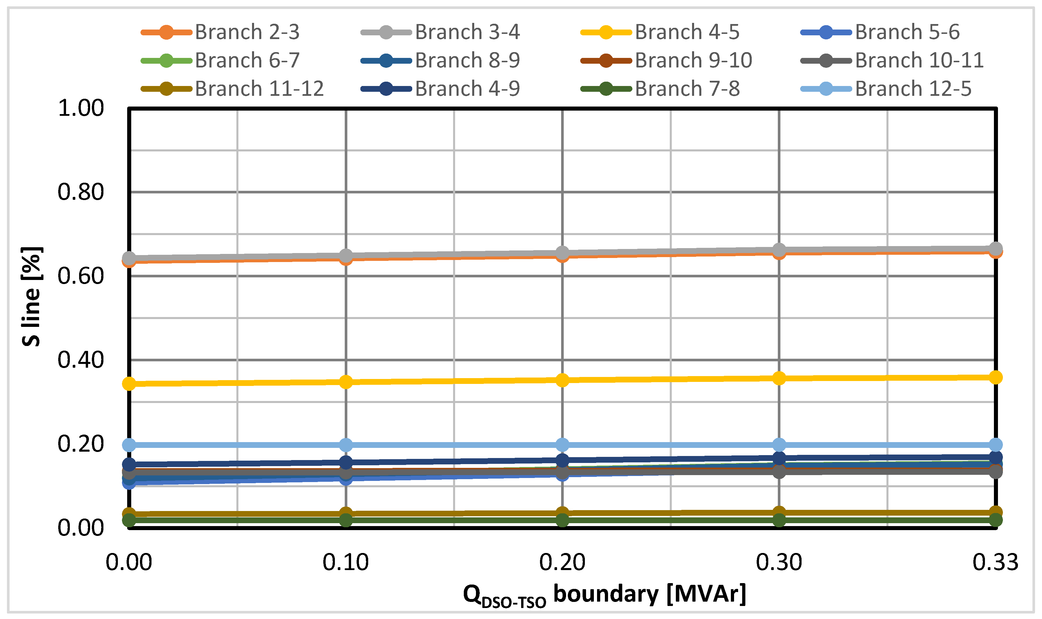
Both TSO and loads demand capacitive reactive power, which is provided by the cheaper providers, WIND7 and WIND8, with no additional PV resources needed. Figure 13 shows the bus voltages and Figure 14 the lines usage when the TSO capacitive needs increase. As can be seen, voltages decrease very slightly, due to the capacitive reactive power voltage generated by the flexible resources, which is coherent with the fact that lines saturation increases also very slightly. Between 0.2 MVAr and 0.3 MVAr, some bus voltages reach their maximum limit and WIND8 reaches the maximum capacitive reactive power it can supply, due to voltages constraints, so the TSO is not able to fulfill all its needs (with a 0.071 MVAr deficit for 0.3 MVAr demanded).

Figure 15 shows the total reactive power injection of the TSO, non-flexible resources, flexible resources and lines contribution, as described in Equation (3) for increasing TSO capacitive needs. In this case, the lines’ reactive power contribution is always a capacitive injection.

Table 4. Reactive power balance for increasing TSO capacitive needs at each market session

	Session 1	Session 2	Session 3	Session 4	Session 5
∆QTSO [MVAr]	0.0000	0.1000	0.1000	0.1000	0.0290
∆QN_flex [MVAr]	1.2747	0.0000	0.0000	0.0000	0.0000
∆QLines [MVAr]	−0.1105	0.0019	0.0023	0.0026	0.0009
∆Qflex_activ. [MVAr]	1.1642	0.1019	0.1023	0.1026	0.0299

shows the reactive power contribution of each player, according to Equations (11) and (12).

Table 5. Incomes and payments for increasing TSO capacitive needs at each market session.

	Session 1	Session 2	Session 3	Session 4	Session 5	Total
QDSO-TSO [MVAr]	0.0000	0.1000	0.2000	0.3000	0.3290
Cap. Price [EUR/MVAr]	3.7000	3.7000	3.7000	3.7000	5.2000
Ind. Price [EUR/MVAr]	0.0000	0.0000	0.0000	0.0000	0.0000
TSO [EUR]	0.0000	0.3700	0.3700	0.3700	0.1508	1.2608
DSO [EUR]	4.3075	0.0070	0.0085	0.0096	0.0047	4.3374
PV4 [EUR]	0.0000	0.0000	0.0000	0.0000	0.0005	0.0005
PV12 [EUR]	0.0000	0.0000	0.0000	0.0000	0.0005	0.0005
WIND7 [EUR]	2.1878	0.3323	0.1606	0.0211	0.1508	2.8525
WIND8 [EUR]	2.1197	0.0448	0.2179	0.3585	0.0036	2.7446

shows the TSO capacitive reactive power needs, the capacitive and inductive market prices, the settlement of each payer according to Equations (13)–(15).

6. Conclusions

This paper proposes a reactive power local market to provide reactive power to the TSO transmission grid from the resources located at the distribution grid of a DSO, where market players can sell and buy capacitive and inductive reactive power, to profit from the market mechanisms. Its main contribution is a new close to real time market design, which allows flexibility providers to supply the reactive power needed by DSO and TSO. The market is based on flexible bids, and clearing guarantees that the DSO grid constraints are respected. The iterative clearing process can include complex bids that provide additional bidding flexibility for more complex assets. This market is a step forward towards TSO-DSO coordination mechanisms in the usage of local distributed flexibility for local and system services.

Indeed, this market is one of the business use cases proposed in the TSO-DSO coordination Flexibility Hub platform of the Portuguese demonstration of the ongoing H2020 EU-SysFlex project, which is a platform to provide TSO-DSO coordination mechanisms. Although liquidity is always a concern in this type of market, it has been designed for a context where most of the resources are located at the distribution grid, the number of traditional reactive power providers has decreased significantly, and generators but also consumers have an increasing active role in the markets, providing all kind of flexibility services, and contributing to the overall grid secure operation.

Since, in the proposed market, the incomes of the market players’ result from netting the sales and purchases of reactive power valuated at the market marginal (uniform) price, it is the responsibility of the market agents to determine the bidding prices that would allow them to recover operation and investments fixed costs. Note, however, that when systems evolve toward optimality, long and short-term costs tend to coincide, and pricing at the variable cost should allow for the recovery of most investments costs (except for the marginal unit, which is the one that sets the market price). However, capacity mechanisms could also be put in place to help recovering assets investment costs. Further analysis should be made, depending on different scenarios of market players, liquidity and needs, to assess the need of additional remuneration mechanisms. Additionally, as in any other market, grid topology, constraints and resources location could lead to market power situations, which should be supervised by the correspondent regulator authority.

The current work is focusing on the analysis of the impact of the grid constraints on the reactive power flexibility that the resources can provide and market power issues, the impact of complex conditions, and the reactive power TSO-DSO coordination mechanism, as well as on the potential need for additional capacity remuneration mechanisms.

References

- Hinz, F. Voltage Stability and Reactive Power Provision in a Decentralizing Energy System. A Techno-Economic Analysis. Ph.D. Thesis, Technische Unuversity, Dresden, Germany, 2017. [Google Scholar]
- Papalexopoulos, A.D.; Angelidis, G.A. Reactive power management and pricing in the California market. In Proceedings of the Melecon 2006—2006 IEEE Mediterranean Electrotechnical Conference, Malaga, Spain, 16–19 May 2006; pp. 902–905. [Google Scholar]
- Ganger, D.; Zhao, J.; Hedayati, M.; Mandadi, A. A review and simulation on real time reactive power spot markets. In Proceedings of the 2013 North American Power Symposium (NAPS), Manhattan, KS, USA, 22–24 September 2013; pp. 1–5. [Google Scholar]
- Zhong, J.; Bhattacharya, K. Reactive power management in deregulated electricity markets-a review. In Proceedings of the 2002 IEEE Power Engineering Society Winter Meeting. Conference Proceedings (Cat. No.02CH37309), New York, NY, USA, 27–31 January 2002; Volume 2, pp. 1287–1292. [Google Scholar]
- Haghighat, H.; Cañizares, C.; Bhattacharya, K. Dispatching Reactive Power Considering All Providers in Competitive Electricity Markets. In Proceedings of the IEEE PES General Meeting, Minneapolis, MA, USA, 27–28 July 2010; pp. 1–7. [Google Scholar]
- Rueda-Medina, A.C.; Padilha-Feltrin, A. Distributed Generators as Providers of Reactive Power Support—A Market Approach. IEEE Trans. Power Syst. 2013, 28, 490–502. [Google Scholar] [CrossRef]
- Zhong, J.; Bhattacharya, K. Reactive power market design and its impact on market power. In Proceedings of the 2008 IEEE Power and Energy Society General Meeting—Conversion and Delivery of Electrical Energy in the 21st Century, Pittsburgh, PA, USA, 20–24 July 2008; pp. 1–4. [Google Scholar]
- Reactive issues—reactive power in restructured markets. IEEE Power Energy Mag. 2004, 2, 14–17. [CrossRef]
- Chicco, G.; Gross, G. Current issues in reactive power management: A critical overview. In Proceedings of the 2008 IEEE Power and Energy Society General Meeting—Conversion and Delivery of Electrical Energy in the 21st Century, Pittsburgh, PA, USA, 20–24 July 2008; pp. 1–6. [Google Scholar]
- Hao, S.; Papalexopoulos, A. Reactive power pricing and management. IEEE Trans. Power Syst. 1997, 12, 95–104. [Google Scholar]
- Khorasany, M.; Azuatalam, D.; Glasgow, R.; Liebman, A.; Razzaghi, R. Transactive Energy Market for Energy Management in Microgrids: The Monash Microgrid Case Study. Energies 2020, 13, 2010. [Google Scholar] [CrossRef]
- Olivella-Rosell, P.; Lloret-Gallego, P.; Munné-Collado, Í.; Villafafila-Robles, R.; Sumper, A.; Ottessen, S.Ø.; Rajasekharan, J.; Bremdal, B.A. Local Flexibility Market Design for Aggregators Providing Multiple Flexibility Services at Distribution Network Level. Energies 2018, 11, 822. [Google Scholar] [CrossRef] [Green Version]
- Zhong, J.; Nobile, E.; Bose, A.; Bhattacharya, K. Localized reactive power markets using the concept of voltage control areas. IEEE Trans. Power Syst. 2004, 19, 1555–1561. [Google Scholar] [CrossRef] [Green Version]
- Zhong, J.; Bhattacharya, K. Toward a competitive market for reactive power. IEEE Trans. Power Syst. 2002, 17, 1206–1215. [Google Scholar] [CrossRef]
- Kargarian, A.; Raoofat, M.; Mohammadi, M. Reactive power market management considering voltage control area reserve and system security. Appl. Energy 2011, 88, 3832–3840. [Google Scholar] [CrossRef]
- Sousa, T.; Hashemi, S.; Andersen, P.B. Raising the potential of a local market for the reactive power provision by electric vehicles in distribution grids. Transm. Distrib. IET Gener. 2019, 13, 2446–2454. [Google Scholar] [CrossRef] [Green Version]
- Zhou, K.; Tang, H.; Liu, T.; Xiong, F.; Wang, L. Reactive power optimization in smart distribution network under power market. In Proceedings of the 2015 5th International Conference on Electric Utility Deregulation and Restructuring and Power Technologies (DRPT), Hu Nan, China, 26–29 November 2015; pp. 663–666. [Google Scholar]
- Caramanis, M.; Ntakou, E.; Hogan, W.W.; Chakrabortty, A.; Schoene, J. Co-Optimization of Power and Reserves in Dynamic T D Power Markets With Nondispatchable Renewable Generation and Distributed Energy Resources. Proc. IEEE 2016, 104, 807–836. [Google Scholar] [CrossRef]
- Batlle López, C.; Gómez San Román, T.; Abbad, R.; Luis, M.; Rodilla Rodríguez, P. Regulation of the Electric Power Industry. Available online: https://repositorio.comillas.edu/xmlui/handle/11531/13739 (accessed on 18 April 2017).
- Haghighat, H.; Kennedy, S. A model for reactive power pricing and dispatch of distributed generation. In Proceedings of the IEEE PES General Meeting, Minneapolis, MA, USA, 27–28 July 2010; pp. 1–10. [Google Scholar]
- Madureira, A.G.; Peças Lopes, J.A. Ancillary services market framework for voltage control in distribution networks with microgrids. Electr. Power Syst. Res. 2012, 86, 1–7. [Google Scholar] [CrossRef] [Green Version]
- Singh, A.; Kalra, P.K.; Chauhan, D.S. New approach of procurement market model for reactive power in deregulated electricity market. In Proceedings of the 2009 International Conference on Power Systems, Kharagpur, India, 27–29 December 2009; pp. 1–6. [Google Scholar]
- Mousavi, O.A. Literature Survey on Fundamental Issus of Voltage and Reactive Power Control; EPF Lausanne-Power System Group: Lausanne, Switzerland, 2011. [Google Scholar]
- Villar, J.; Aguiar, J.; Retorta, F.; Silva, B.; Fulgêncio, N.; Lopes-Filipe, N.; Marques, M.; Louro, M.; Moreira, J.; Soares, A. Flexibility Hub-Multi Service Framework for Coordination of Decentralized Flexibilities. In Proceedings of the 25th International Conference on Electricity Distribution, CIRED 2019, Madrid, Spain, 3–6 June 2019. [Google Scholar]
- ‘Documents—EU-SysFlex’. Available online: https://eu-sysflex.com/documents/ (accessed on 30 September 2019).
- Carpentier, J. Contribution a. ‘l’etude du Dispatching Economique. Bull. Soc. Francaise Electr. 1962, 3, 431–447. [Google Scholar]
- Megiddo, N. (Ed.) Progress in Mathematical Programming: Interior-Point and Related Methods; Springer: New York, NY, USA, 1989; ISBN 978-1-4613-9619-2. [Google Scholar]
- Quintana, V.H.; Torres, G.L.; Medina-Palomo, J. Interior-point methods and their applications to power systems: A classification of publications and software codes. IEEE Trans. Power Syst. 2000, 15, 170–176. [Google Scholar] [CrossRef]
- Low, S.H. Convex Relaxation of Optimal Power Flow—Part I: Formulations and Equivalence. IEEE Trans. Control Netw. Syst. 2014, 1, 15–27. [Google Scholar] [CrossRef] [Green Version]
- AlRashidi, M.R.; El-Hawary, M.E. Hybrid Particle Swarm Optimization Approach for Solving the Discrete OPF Problem Considering the Valve Loading Effects. IEEE Trans. Power Syst. 2007, 22, 2030–2038. [Google Scholar] [CrossRef]
- Benchmark Systems for Network Integration of Renewable and Distributed Energy Resources. Available online: https://e-cigre.org/publication/ELT_273_8-benchmark-systems-for-network-integration-of-renewable-and-distributed-energy-resources (accessed on 25 September 2019).
- Kirby, B.; Hirst, E. Ancillary Service Details: Voltage Control; Oak Ridg National Laboratory: Oak Ridge, TN, USA, 1997.
Figure 1.
Market agents and actions sequence.