Financial Liberalisation, Political Stability, and Economic Determinants of Real Economic Growth in Kenya

Abstract

This study aimed to analyse financial liberalisation, political stability, and economic determinants of Kenya’s real economic growth using time series data over the period of 1970–2016. The authors specified quadratic and interactive models to be estimated by employing a quantile regression analysis. The traditional and quantile unit root test was used in testing the stationarity issue. The co-integration findings indicated that the capital account openness and financial development impede on real economic growth; and the political stability also had potential influence on the real economic growth of Kenya. Interestingly, there is a nonlinear U-shape link between financial development and real economic growth that undermined the real economic growth at its onset, but as it advanced, it enhanced the growth of the country in the long run. The policymakers should ensure that the capital account is more liberalised so that it will continue to stimulate the financial development. In the same way, the liberalisation of the domestic financial market should be taken in earnest to overcome the negative effects of financial repression in totality, while maintaining the stable political atmosphere.

1. Introduction

It is theoretically and empirically established that financial development has a significant role in the growth of an economy. Bhattacharyya [1] made efforts to show the various ways in which financial market development enhances economic growth. However, they emphasise that an advanced domestic financial system is essential for the substantial growth of foreign capital and trade that enhanced economic growth. To avoid the undesirable impact on the economy, developing countries did move to improve their financial system in order to meet the required standards for integration into the global economy for the flow of foreign direct investment (FDI) and equity. The benefits of financial liberalisation on output growth in the developing economies are in three dimensions, according to Ibrahim [2]. First, the enhancement of specialisation in production, opportunities to share risks, and hedge portfolio of investors from shocks that can hinder their participation in high return projects. Second, financial liberalisation enhances the global flows of capital resources to fund investment in less developed countries, given their marginal productivity. Third, it paves a way for the penetration of more foreign banks that are efficient to diversify domestic opportunities, which reduces risk and smooths consumption.

This study attempts to explore the linkage between capital account openness, financial development, trade openness, government expenditure, and political stability; as well as its impact on real Gross Domestic Product (GDP) per capita using the availability of the time series data for 1970 until 2016 for the economy of Kenya. The country has made a deliberate and steady important financial market reform program as far back as the early 1980s [3]. This is to pave their way into the global capital market to improve trade and investment flows. The reforms include interest rate liberalisation, bank denationalisation, liquidation, restructuring, privatisation, etc. Similarly, in 2008, the Kenya Vision 2030 aimed to achieve a 10% GDP growth rate per annum over 25 years, which was the fashion to improve the domestic financial market [4]. These changes are hoped to improve and liberalise the domestic financial system and attract more foreign capital flows. The available statistical data shows that FDI inflows into the Kenya economy has increased recently, and there is an emergence of portfolio equity. Capital flows have grown over the years at US 9578 million in 1991 to US 40,029 million in 2014 [5]. Indeed, this is interesting for the economy as there is a lag between savings and the investment rate.

Table 1. Kenya’s macroeconomic performance indicators.

Period	GDP Per Capita Growth (Annual %)	Domestic Credit (% GDP)	Foreign Direct Investment (% GDP)	Gross Domestic Savings (% GDP)	Gross Capital Formation (% GDP)	Total Trade (% GDP)
1970–1979	3.265	17.926	0.8167	20.202	23.223	63.035
1980–1989	0.412	19.677	0.424	19.308	23.171	56.290
1990–1999	−0.822	22.069	0.605	14.417	18.314	58.988
2000–2009	0.774	25.056	0.513	7.147	18.047	56.009
2010–2016	3.271	31.431	1.649	7.127	20.897	51.247

shows that the GDP per capita growth in annual % declined from a high point of 3.265 to −0.822 between the period 1970–1979 and 1990–1999, respectively, then started increasing in the period 200–2009 and 2010–2016 from 0.774 to 3.271, respectively. This could be due to the sustained increase in domestic credit as a % of GDP and FDI, which indicated to be at a high point, especially in the period 2010–2016. However, for gross domestic savings as a % of GDP, it depicts a shortfall to the gross capital formation as a % of GDP in all the periods, indicating that savings are augmented by FDI and other sources in the financing investment in Kenya. Total trade as a % GDP did not reveal an increasing trend, it swung, and remained at a relatively high level, meaning it could have an impact on the economy.

2. Literature Review

In the financial liberalisation policies, trade openness should precede capital account liberalisation [6]. When the economy is fully liberalised, economic growth is feasible because of the bridge created in the savings and the foreign exchange gap. Furthermore, the liberalisation of capital account allows for an international portfolio diversification, which domestic market agents enjoy in diversifying country-specific risks that cannot be diversified under capital account restriction. Omoruyi [7] has viewed capital account openness as the process of removing restrictions from international transactions related to the movement of capital. With financial liberalisation, the level of competition that causes convergence prices increases, as well as an increase in the firm’s output and the allocation of capital to a lucrative investment [8]. However, despite the theoretical claims of the impact of financial liberalisation, empirically, there is no firm conclusion. The lack of that claim in developing countries is because of an ‘allocative puzzle’ [9].

Gehringer [10] examined the impact of financial openness on economic growth on two channels: The manufacturing and service industry in eight European countries. The results indicated that the impact on manufacturing is more than the service industry on economic growth. Bekaert et al. [11] contributed that the capital account openness spurs economic growth, but the impact relies on the quality of the institution. In another perspective, Ibrahim [2] stated that although the capital account openness impacts economic growth, it depends on the level of economic development. This, in a nutshell, indicates that the more the economy develops, the better the impact of capital account openness on economic growth. However, Hye and Wizarat [12] do not find a significant impact between capital account openness and economic growth. This is a similar finding of Ahmed and Mmolainyane [13] who reported that the capital account openness impedes economic growth, but it is positive and significantly correlated with financial development. This means that the capital account openness can enhance economic growth through financial development. Other researchers, such as Berthelemy and Demurger [14], revealed that the capital account openness promotes the transfer of technology and managerial skills, which increase production output.

On the contrary, other studies mainly were not able to find a definite relationship between financial liberalisation and growth in developing economies. They indicated that the growth side of the lagging economies could not be identified significantly. Gourinchas and Jeanne [9], Alfaro et al. [15], and Prasad et al. [16] studied the impact of financial openness fields. The results of those studies disagreed with the assertion that it stabilises the fluctuations in consumption in developing economies. In addition, Bussiere and Fratzscher [17] do not find a link connecting capital account openness to economic growth. However, the findings of that study concluded that the capital account openness merely causes excess borrowing in the short term that creates booming and, in the midterm, brings recession. However, the importance of capital account openness in developing economies cannot be ignored by Rajan and Zingales [18] on the simultaneously opened hypothesis of capital and trade effect on financial development.

Meanwhile, Onanuga [19] demonstrated that the simultaneous opening of the capital account and the trade spurred the sophistication of the domestic financial market in Nigeria. The results of that study argue that if either capital account is opened and trade is closed, the impact will be detrimental to economic growth. Mubi [20] found that the interaction of capital inflow with trade openness spurs economic growth through financial development using the ARDL estimates in Nigeria. However, Gossel and Biekpe [21] found that the capital inflow hindered economic growth in South Africa over the period 1995 to 2011. This is evidence that more studies are needed in African countries, especially Kenya, to ascertain the effect of capital openness on economic growth as there is a dearth of empirical studies on that.

On the other hand, McKinnon [22] and Shaw [23] postulated that countries that adopted financial liberalisation policies might become more equipped and matured as savings and investment will increase to overcome future growth challenges. This is an indication of experiencing the U-shape curve relationship between financial development and growth. Shen et al. [24], however, found the contrary, as there was an inverted U-shape between the banking sector development and economic growth. This was supported by Yang and Liu [25] and Ibrahim and Alagidede [26] that found a U-shape relationship between financial development and economic growth. Similarly, Adeniyi and Oyinlola [27] contributed that financial development negatively impacts economic growth, which reverses itself accounting for threshold-type effects, but the impact is infinitesimal.

A recent study by Ashraf [28] suggested that the higher trade openness is vital for financial development as it increases the volume and reduces the cost and risk of bank credit because of the increase in demand for finance, the liberalisation in the domestic financial sector reforms, and the diversification of lending opportunities created through the higher trade openness. Notwithstanding, Redmond and Nasir [29] found that trade openness and financial development had significant negative impacts of economic development. Atil et al. and Mercado [30] opined that the abundance of natural resources and financial development are positively correlated, and economic growth stimulates financial development, but on the contrary, economic globalisation is a bane of financial development. This economic globalisation can be the causal factor that the financial development undermines economic growth as it causes inflows of capital in some economies that do not stay long to impact the economies, which Gourinchas and Jeanne [9] argued as the detrimental factor to the economy.

Political institutions are critical to the growth of an economy in a financial reform policy, and this is because it provides the conducive environment for financial development to promote growth [31]. In the same vein, Bhattacharyya [32] postulated that the democratic institution is an incremental process, not a one-off phenomenon. Countries with a more democratic system have a more market-based financial system. The quality of political institutions when setting at the optimal threshold level minimised political risk, and by that, economic growth can be achieved through financial development [33]. Thus, the economy gains from financial development when the political system is above a threshold, and it is relatively stable. Nevertheless, if there is political instability, it affects the inflows and sustainability of foreign investors, as any shock and sudden changes in the political arena mar all their investment outlets. This causes ’stops’ of an extreme state of lower capital inflows in an economy, which is the opposite of ‘surges’ [34].

The remainder of this paper is structured. Thus, Section 2 is the literature review and Section 3 captures the data and model specification. Section 4 presents the empirical results, while Section 5 gives the concluding remarks.

3. Data and Model Specification

Table 2. Data sources and variable descriptions.

Variables	Description	Data Sources
RGDP	Represents the real GDP per capita measures in US currency at the 2010 constant basic price after taking the deflator effects.	World Development Indicators (WDI)
COP	Represents the capital account openness which is measured in US currency. It is the sum of total foreign assets and total foreign liabilities (% of GDP).	External Wealth of Nations Mark II Database.
FD	Represents the financial development index measured using the Principle Component Analysis (PCA) that includes the broad money, domestic credit to the private sector, domestic credit to the private sector by banks, and domestic credit provided by the financial sector (all as a % of GDP).	World Development Indicators (WDI)
TOP	It is indicating the total countries volume of export and import as measured in US currency (% of GDP).	World Development Indicators (WDI)
GEX	Represents the total government expenditure on final goods and services, excluding military expenditure (% of GDP).	World Development Indicators (WDI)
PST	Represents the stability of political institutions of the country measured using a specific formulation.	Centre for Systemic Peace

presents the variable description and the sources of data utilized in the study.

In Figure 1, we show the estimated series of plots within the estimation period of this study. We begin our analysis from the 1970s, and some of the series appears with a robust structural break in the middle of the 1990s which may well be due to changes in Kenya’s macroeconomics fundamentals, such as the FDI, financial development, and inflation. Hence, to avoid bias estimation, this plot urgently needs a structural break analysis to identify the structural break effects of each series which contains useful information for policymakers. The relationship between the variables was tested using the following equations:

$$RGDP=f\left(COP, FD,TOP,GEX,PST,F{D}^2\right)$$

(1)

where all the variables stated in Table 2 are gathered from [5,35,36,37], while FD² represents the squared value of financial development. The variable RGDP per capita is the proxy of economic growth as used by [27,31,37,38] in their studies shown clearly in Equation (1). While Equation (3) concentrates on the interactive effects between the capital account and trade openness with the financial development series:

$$RGDP=a_0+{\beta }_{1}COP+{\beta }_{2}FD+{\beta }_{3}TOP+{\beta }_{4}GEX+{\beta }_{5}PST+{\beta }_{6}F{D}^2+\mu$$

(2)

$$RGDP=a_0+{\beta }_{1}COP+{\beta }_{2}FD+{\beta }_{3}TOP+{\beta }_{4}GEX+{\beta }_{5}PST+{\beta }_6\left(FD\times COP\right)+{\beta }_7\left(FD\times TOP\right)+\mu$$

(3)

Notably, most of the time series data always faced a unit root problem, such as the random walk, cycle, and trend effects, as shown in Figure 1. This causes spurious regression estimation among the series in the study. Thus, the unit root issue needed to be addressed in the series. Prior to the empirical analysis, all the series are transformed into a natural logarithm. The unit root tests employed are the traditional unit root tests, such as the [39,40] as a traditional unit root and Perron’s test for unknown break determination [41].

To capture the long-run co-integration, we used the long-run equation by emphasising the Dynamic Ordinary Least Square (DOLS) and Fully Modified Ordinary Least Square (FMOLS) estimations proposed by the [42,43] test, respectively. The DOLS estimation will address the asymptotic bias of the estimation series, which contains the normal OLS estimation by including the leads and the lags of the first difference of the series. After confirming the long-run co-integration relationship, a robust test of combined co-integration developed by Bayer and Hanck [44] was employed. This is better than the Johansen [45] on the Johansen Maximum-Eigenvalue test that allows more than one co-integration relationship. An improved joint test-statistics by Bayer and Hanck [44] gives room for the combinations of others to provide conclusive findings in a multidimensional manner. Thus, it was applied in the study. The combination of the individually computed p-value following Fisher’s formula is as follows:

$$EG-JOH=-2[\ln \left(E{G}_p\right)+\left(JO{H}_p\right)]$$

(4)

$$EG-JOH-BO-BDM=-2 \left[\ln \left(E{G}_p\right)+\left(JO{H}_p\right)+\left(B{O}_p\right)+\left(BD{M}_p\right)\right]$$

(5)

where the p sign indicates the probability value of each individual test of co-integration through the Bayer and Hanck’s combined co-integration estimation. The criteria for the rejection of the null hypothesis of co-integration is for the critical values to be lower than the Fisher’s statistics. This type of co-integration test has an advantage, according to Polat et al. [46], Rafindadi [47], and Bekun [48] who employed it in some African studies. This technique is the combination of the Engle and Granger [49] and the Johansen [50], the error correction F-test of Boswijk [51], and the error correction t-test of Banerjee et al. [52]. Moreover, the BH relies on the order of one level of integration of the series, and one-off determination of the stated techniques. The EG-JOH in Equation (4) represents the combination of the Engle and Granger and Johansen probability value. While the EG-JOH-BO-BDM in Equation (5) is the combination of the Engle and Granger, Johansen, Boswijk, and the Banerjee probability value of those co-integration tests.

The Koenker and Xiao [53] quantile unit root test stresses on the different quantile effects not minding that the deterministic trend effect was employed in this study. This was because of its accuracy, flexibility, and the reduction of estimation uncertainty. Furthermore, Bolat et al. [54] stressed the advantages of the quantile unit root test over the traditional unit root test when the shock displays a heavy-tailed behaviour. This technique explores the speed of mean reversion in a series under different magnitudes and signs of shock. To put it succinctly, it captures possibly different mean-reverting patterns by explicitly testing for a unit root at different quantiles. The quantile unit root test depends on the conditional quantile auto-regression (AR) model for the RGDP as follows:

$$Q_{RGDP}\left(\tau |F_t\right)={\alpha }_0\left(\tau \right)+a_1\left(\tau \right)RGDP+{\displaystyle \sum }_{j=1}^q{\alpha }_{j+1}\left(\tau \right)\mathsf{\Delta }RGDP$$

(6)

where $Q_{RGDP}\left(\tau |F_t\right)$ is a conditional distribution function of the $RGDP$ series to a level $r \in \left(0,1\right),$ and the $F_t$ series stands for the accumulated information up to the time frame of t. The null hypothesis is $H_0:a_1\left(\tau \right)=1$ for the given quantile $\left(\tau \right)$. The authors of [53] introduce the Kolmogorov-Smirnov test to indicate the unit root properties of a range of quantiles not only dwelling on some quantiles as follows:

$$QKS=\sup \left|{\tau }_n\left(\tau \right)\right|$$

(7)

where ${\tau }_n\left(\tau \right)$ stands for the t ratio and is computed at ${\tau }_i\in \mathsf{\Gamma }$; therefore, the QKS test is formed using the maximum over $\Gamma$. The distribution of the ${\tau }_n\left(\tau \right)$ is limited. The QKS test depends on the parameter, which is a nuisance. The next step is the quantile unit root test and the quantile regression. As the dependent variable is the RGDP and the independent variable is the COP. The expression of the conditional quantile regression function ${\tau }^{th}$ is stated as follows:

$$Q_{RGDP}\left(\tau |COP\right)=\inf \left\{b|F_{RGDP}\left(COP\right)\ge \tau \right\}={\displaystyle \sum }_K{\beta }_K\left(\tau \right)CO{P}_K={\chi }^1 \beta \left(\tau \right)$$

(8)

where $F_{RGDP}\left(COP\right)$ is the function of the conditional distribution of $RGDP$ and $COP$ series, while $\beta \left(\tau \right)$ is the dependence relationship of the regressed series of the specified quantiles $\left(\tau \right)$. The authors of [55] estimated that $\beta \left(\tau \right)$ for each quantile is calculated through the minimisation of the weighted deviation between the series estimated as follows:

$$\beta \left(\tau \right)=\mathrm{Argmin}{\displaystyle \sum }_{t=1}^T\left(\tau -1_{\left\{yt<{\chi }_t^{\prime } \beta \left(\tau \right)\right\}}\right)$$

(9)

The coefficient can vary across quantile $\left(\tau \right)$ and it can be extended through calculating ${\beta }_K^{\left(\tau \right)}$ when $\tau$ equals 0.10, 0.25, 0.50, 0.75, and 0.90; and K represents the number of parameters including the intercept. The aim is to indicate the different effects on the dependent variable by the independent variables across the quantile. Therefore, the quantile regression was formulated as follows:

$$Q_{RGDP}\left(\tau |X\right)={\alpha }_0^{\left(\tau \right)}+{\alpha }_1^{\left(\tau \right)}COP+{\alpha }_2^{\left(\tau \right)}FD+{\alpha }_3^{\left(\tau \right)}TOP+{\alpha }_4^{\left(\tau \right)}GEX+{\alpha }_5^{\left(\tau \right)}PST+a_{6}F{D}^2+{\in }_t^{\left(\tau \right)}$$

(10)

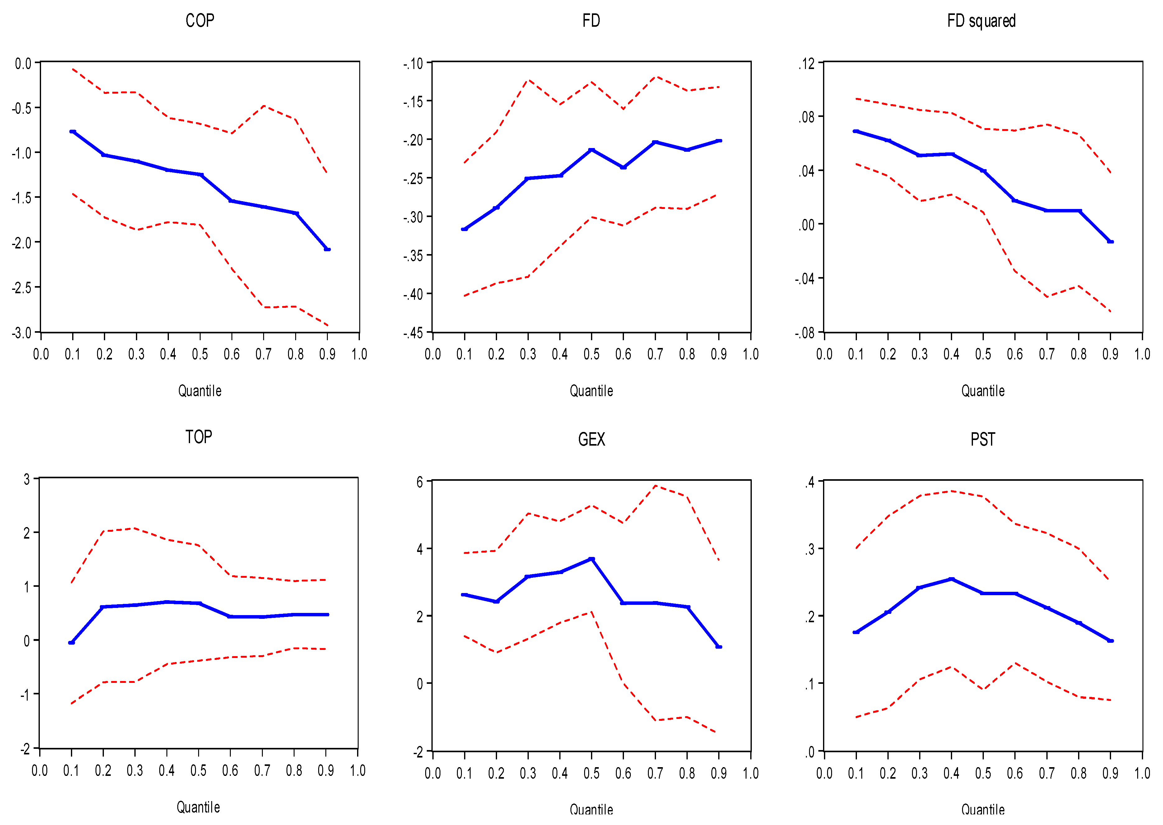
4. Empirical Results

In

Table 3. Summary of statistics.

Variables	RGDP	COP	FD	TOP	GEX	PST
Mean	7.740	−0.450	−0.001	4.043	2.801	1.977
Median	7.170	−0.452	−0.105	4.024	2.820	2.197
Maximum	9.148	0.230	4.102	4.312	2.986	3.296
Minimum	6.698	−0.891	−3.263	3.604	2.587	0.000
Std. Dev.	0.952	0.246	1.900	0.133	0.108	0.997
JB (p-values)	0.051	0.743	0.383	0.079	0.216	0.125

, the descriptive statistics are presented. The Jarque-Bera (JB) statistics show that the RGDP per capita and TOP are not normally distributed, and the financial development and political stability series have the highest spread. The most volatile series in the financial development is with 1.9 standard deviations, while the capital account openness is the least with 0.246 standard deviations.

The ADF, PP, and Perron’s tests of unit root results are reported in

Table 4. The unit root test results.

Variables	At Level			At First Difference
	ADF	PP	Perron	ADF	PP	Perron
RGDP	−1.144	−1.571	−3.164 (TB: 2004)	−4.714 *	−4.672 *	−7.634 * (TB: 1993)
COP	−1.563	−1.465	−3.350 (TB: 2004)	−7.813 *	−7.813 *	−10.888 * (TB: 1993)
FD	−1.435	−1.212	−4.602 (TB: 2009)	−8.562 *	−8.842 *	−9.828 * (TB: 1995)
TOP	−2.936	−2.936	−3.651 (TB: 1992)	−7.205 *	−7.307 *	−7.644 * (TB: 1993)
GEX	−3.083	−3.076	−3.541 (TB: 1990)	−6.550 *	−8.170 *	−7.550 * (TB: 2006)
PST	−2.548	−2.565	−2.874 (TB: 2006)	−6.149 *	−6.184 *	−8.057 * (TB: 1997)

Note: * indicate significance levels at 1% level and T_B represents the break year of the [41] unit root test.

, which indicates that all series are stationary at the first difference I(1). These reject the null hypothesis of no stationarity. Moreover, the single break date of the RGDP per capita, according to Perron’s [41] unit root test with unknown breaks is in 2004. While in 1992 and 1993, the RGDP growth of Kenya falls massively as a result of the decline in manufacturing activities. Therefore, we found that there is an unknown structural break faced by TOP and GEX in 1992 and 1990, respectively. The fiscal indiscipline and macroeconomic imbalances, as well as the imposition of import licenses and foreign exchange control, caused the slow growth in export. This necessitated the adoption of financial reform policies in the early 1990s in Kenya [4].

The results of the quantile unit root test were depicted in

Table 5. Quantile unit root test results.

Variables	Lower Quantile	Middle Quantile		Upper Quantile
	$\mathit{\tau }=0.25$	$\mathit{\tau }=0.50$	$\mathit{\tau }=0.75$	$\mathit{\tau }=0.90$
Panel 1: RGDP
$\alpha \left({\tau }_0\right)$	−0.101 ** (0.050)	−0.015 (0.399)	0.024 (0.376)	0.094 (0.192)
$\alpha \left({\tau }_1\right)$	0.980 (0.353)	0.985 (0.394)	0.977 (0.344)	0.997 (0.487)
$\alpha \left({\tau }_n\right)$	−0.392 (0.600)	−0.601 (0.570)	−1.077 (0.430)	−0.339 (0.560)
QKS test	1.405 [4.658]
Panel 2: COP
$\alpha \left({\tau }_0\right)$	−0.077 * (0.001)	0.011 (0.371)	0.045 *** (0.079)	0.113 ** (0.021)
$\alpha \left({\tau }_1\right)$	0.845 ** (0.048)	0.884 (0.158)	0.854 (0.101)	0.884 (0.288)
$\alpha \left({\tau }_n\right)$	−2.265 ** −(0.050)	−1.625 (0.270)	−2.228 ** (0.040)	−0.428 (0.610)
QKS test	2.337 [4.658]
Panel 3: FD
$\alpha \left({\tau }_0\right)$	−0.413 (0.134)	0.163 (0.285)	0.539 ** (0.023)	0.981 ** (0.015)
$\alpha \left({\tau }_1\right)$	0.874 (0.157)	1.016 (0.440)	1.008 (0.471)	0.933 (0.373)
$\alpha \left({\tau }_n\right)$	−1.349 (0.160)	0.195 (0.980)	0.084 (0.950)	−0.377 (0.700)
QKS test	2.458 [4.101]
Panel 4: TOP
$\alpha \left({\tau }_0\right)$	−0.085 * (0.000)	−0.021 (0.221)	0.050 * (0.008)	0.090 ** (0.046)
$\alpha \left({\tau }_1\right)$	0.537 * (0.000)	0.614 * (0.004)	0.707 ** (0.011)	0.627 (0.105)
$\alpha \left({\tau }_n\right)$	−2.365 ** (0.040)	−2.337 *** (0.090)	−1.422 (0.320)	−0.892 (0.370)
QKS test	2.401 [4.120]
Panel 5: GEX
$\alpha \left({\tau }_0\right)$	−0.045 * (0.003)	−0.009 (0.257)	0.013 (0.152)	0.052 * (0.000)
$\alpha \left({\tau }_1\right)$	0.872 (0.163)	0.976 (0.413)	0.889 (0.164)	0.888 (0.161)
$\alpha \left({\tau }_n\right)$	−0.857 (0.390)	−0.206 (0.830)	−1.143 (0.409)	−0.678 (0.410)
QKS test	1.581 [5.342]
Panel 6: PST
$\alpha \left({\tau }_0\right)$	0.115 ** (0.041)	0.150 * (0.000)	0.200 * (0.000)	0.287 * (0.000)
$\alpha \left({\tau }_1\right)$	0.931 *** (0.098)	0.877 * (0.000)	0.840 * (0.000)	0.795 * (0.000)
$\alpha \left({\tau }_n\right)$	−0.177 (0.190)	−10.420 * (0.000)	−7.553 * (0.000)	−9.234 * (0.000)
QKS test	10.420 [4.116]

Note: *, **, and *** indicate significance levels at 1, 5, and 10%, respectively. QKS denotes the Kolmogorov-Smirnov test statistic and the numbers in ( ) and [ ] represents the probability values of QKS critical values, respectively.

. These include the constant term value $\alpha \left({\tau }_0\right)$, the coefficient of autoregressive value $\alpha \left({\tau }_1\right)$, the value of the QKS test, and the probability of the values. To start with, the test of QKS gives a mean-reverting behaviour of each variable. It illustrates evidence in favour of mean-reverting in political stability at the 10% level of significance. Subsequently, the behaviour of the variables in a specified quantile was examined through the estimated value of the intercept $\alpha \left({\tau }_0\right)$ and the coefficient of autoregressive $\alpha \left({\tau }_1\right)$. The intercept $\alpha \left({\tau }_0\right)$ gives the size of the shock observed within the quantiles that affect the series.

In the case of RGDP, it has a shock of significant extent in the lower quantile, while in COP and TOP the shock is at the lower and upper quantiles. As for FD, the shock is very high at the upper quantiles between the range of 0.539 to 0.981. For GEX, the shock is the lowest at the lower and upper quantile, while the shock in PST is the most concentrated running from 0.115 to 0.287 across all the quantiles. These results show that FD experienced the highest shock level to the point that it moves far away from its long-run equilibrium level at about 0.981 units. The $\alpha \left({\tau }_1\right)$ value estimated is less than one (1) in all variables, but the probability value that rejects the non-stationarity of COP is at the lower quantile, while TOP rejects the unit root null up to a 75% quantile. Indeed, PST rejects the non-stationarity across all quantiles; in other words, it displays a mean reversion.

We have performed the tests of co-integration since all series faced I(1) based on the ADF and PP test of unit root, but for Perron’s test of unit root with an unknown break date, only PST is integrated at I(0). The results of the OLS, FMOLS, and DOLS techniques are compared. Both DOLS and FMOLS gave good and significant estimates. The results in

Table 6. Co-integration test results.

Variables	Long-Run Estimates
	OLS	FMOLS	DOLS
COP	−1.323 * (0.000)	−1.384 * (0.000)	−1.578 * (0.000)
FD	−0.247 * (0.000)	−0.252 * (0.000)	−0.226 * (0.000)
FD2	0.038 *** (0.073)	0.041 * (0.004)	0.043 ** (0.048)
TOP	0.310 (0.325)	0.503 (0.136)	0.807 (0.206)
GEX	3.122 * (0.000)	2.999 * (0.000)	2.892 * (0.006)
PST	0.213 * (0.000)	0.212 * (0.000)	0.205 ** (0.015)

Note: *, **, and *** indicate significance levels at 1, 5, and 10% respectively. Values in ( ) represent the probability values.

showed that COP and FD have a negative effect on RGDP, particularly, GEX and PST have a positive impact on the normalised RGDP. The result of the negative effect of capital account openness does not agree with [2], as political stability is statistically significant to economic growth. Interestingly, the FD² coefficient is positive and statistically significant, according to the OLS, FMOLS, and DOLS techniques. The positive sign of the FD squared series indicated a U-shape curve between financial development and RGDP per capita. This indicates that there was little advancement of financial development in Kenya towards the real GDP per capita after the attainment of the threshold, but the impact is very small between the range of 0.038 to 0.043. This agreed with the results of Adeniyi et al. [27] in Nigeria that reported a nonlinear threshold type-effect between financial development and economic growth. The TOP series has a positive relationship with economic growth, but not significant, while GEX and PST showed a significant positive relationship with economic growth. For GEX, it gave a high magnitude indicating that the economy is more driven by the public sector than the private sector. On the other hand, the PST caused economic growth in Kenya, depicting that the regime change has no negative impact on the economy.

The combined co-integration of the Bayer and Hanck [44] test facilitates the establishment of the multidimensional co-integration link of the study series. In

Table 7. The Bayer and Hanck (2013) co-integration test results.

Estimated Models	EG-JOH	EG-JOH-BO-BDM	Decision
$RGDP=f\left(COP,FD,TOP, GEX,PST \right)$	55.384 *	70.781 *	Yes
$COP=f\left(RGDP,FD,TOP, GEX,PST\right)$	55.310 *	110.595 *	Yes
$FD=f\left(COP,RGDP,TOP, GEX,PST\right)$	56.116 *	76.142 *	Yes
$TOP=f\left(COP,FD,RGDP,GEX,PST\right)$	56.922 *	112.185 *	Yes
$GEX=f\left(COP,FD,TOP,RGDP,PST\right)$	55.670 *	112.459 *	Yes
$PST=f\left(COP,FD,TOP,RGDP,GEX\right)$	55.349 *	71.000 *	Yes
Significant level	Critical values
1%	15.701	29.85
5%	10.419	19.888
10%	8.242	15.804

Note: * indicate significance levels at 1% level and the optimal lag length selection is based on the AIC (k = 4).

, the estimated equations reject the null hypothesis of a no combined co-integration condition, significantly at the 1% level. This proves that a long-run relationship appeared between the estimated series, indicating the existence of equilibrium of the real GDP per capita and its determinants. Moreover, Polat et al. [46], Rafindadi [47], and Bekun [48] also equally discovered similar results in their studies.

In

Table 8. The bootstrap quantile regression.

Variables	Quantile Bootstraps Estimation
	$\mathit{\tau }=0.10$	$\mathit{\tau }=0.25$	$\mathit{\tau }=0.50$	$\mathit{\tau }=0.75$	$\mathit{\tau }=0.90$
COP	−0.774 * (0.035)	−1.113 * (0.005)	−1.249 * (0.000)	−1.616 * (0.004)	−2.084 * (0.000)
FD	−0.317 * (0.000)	−0.282 * (0.000)	−0.214 * (0.000)	−0.209 * (0.000)	−0.202 * (0.000)
FD2	0.069 * (0.000)	0.061 * (0.000)	0.039 ** (0.017)	0.011 (0.715)	−0.013 (0.633)
TOP	−0.055 (0.924)	0.761 (0.302)	0.681 (0.220)	0.418 (0.219)	0.468 (0.161)
GEX	2.621 * (0.000)	2.437 * (0.006)	3.691 * (0.000)	2.360 (0.164)	1.076 (0.420)
PST	0.175 * (0.009)	0.213 * (0.009)	0.233 * (0.003)	0.210 * (0.000)	0.163 * (0.001)
Pseudo R2	0.699	0.727	0.793	0.783	0.747
Sparsity	1.006	0.800	0.724	0.762	1.023
Prob. (Quasi-LR)	0.000	0.000	0.000	0.000	0.000

Note: * and ** indicate significance levels at 1 and 5% levels, respectively. Figures in ( ) are probability values.

, the bootstrap quantile regression at quantile 0.10, 0.25, 0.50, 0.75, and 0.90 is presented. From the estimated results, COP has a negative effect on the real GDP per capita with coefficients ranging between −0.77 and −2.084. This is in line with the ‘allocative puzzle’ of [9] that instead of capital inflow into the developing economies, is the outflow of capital from the developing economies. The coefficient of financial development produces a threshold type effect, as it was negative before, and after the threshold, it turned positive and statistically significant at the lower and middle quantile (10th, 25th, and 50th). It means that financial development stimulates growth at the advanced stage. The financial liberalisation policies of 1991 could be the factor that contributed to the square of financial development to spur economic growth. However, due to the global financial crisis between 2007 and 2008, which stifled the Kenya domestic financial market development, the impact of the square financial development impedes economic growth from the 75th to 90th quantiles.

TOP hindered RGDP at the 10th quantile only, but at upper quantiles, it has a positive relationship with economic growth, although not significant. Since the COP and FD could not enhance RGDP, it is a sign that the TOP chances to stimulate RGDP were slimmed. GEX is positive and statistically significant from the 10th to 50th quantiles, but not at the higher quantile. This can be a result of the economic imbalance between 2007 and 2008. Mwega [4] stated that apart from the global financial crisis of that period, the Kenya economy was affected by the post-election crisis of 2007/2008. In addition, adverse weather affected agricultural activities, which undermined the implementation of the first and the second Medium Term Plan of the period 2008–2017 of Kenya’s Vision 2030 Development Plan.

Table 9. The bootstrap quantile regression with iterative effects.

Variables	Quantile Bootstraps Estimation
	$\mathit{\tau }=0.10$	$\mathit{\tau }=0.25$	$\mathit{\tau }=0.50$	$\mathit{\tau }=0.75$	$\mathit{\tau }=0.90$
COP	−0.788 (0.175)	−1.695 * (0.000)	−1.483 * (0.000)	−1.294 * (0.001)	−1.454 * (0.003)
FD	3.017 * (0.015)	1.079 ** (0.034)	0.841 (0.221)	0.735 (0.324)	0.053 (0.957)
TOP	0.510 (0.570)	0.530 (0.135)	0.440 (0.345)	0.520 (0.171)	0.598 (0.126)
GEX	3.556 * (0.007)	3.038 * (0.000)	3.352 * (0.000)	2.915 ** (0.013)	2.001 (0.117)
PST	0.254 (0.140)	0.433 * (0.000)	0.320 * (0.000)	0.220 * (0.003)	0.178 * (0.019)
(FD × COP)	0.333 (0.560)	0.430 * (0.009)	0.338 (0.136)	0.245 (0.177)	0.365 (0.247)
(FD × TOP)	−0.767 * (0.036)	−0.259 ** (0.050)	−0.209 (0.240)	−0.203 (0.235)	−0.023 (0.915)
Pseudo R2	0.644	0.701	0.803	0.795	0.750
Sparsity	1.312	0.612	0.664	0.729	1.111
Prob. (Quasi-LR)	0.000	0.000	0.000	0.000	0.000

Note: * and ** indicate significance levels at 1 and 5% levels, respectively. Figures in ( ) are probability values.

illustrates the bootstrap quantile regression under interactive effects. The results presented indicate that financial development is statistically significant to economic growth at the 10th and 25th quantiles. This is contrary to model 1, but because it is an interactive model, FD spurs RGDP. Uddin et al. [56] agreed that financial development influences economic growth in Kenya. It is further validated with the complimentary coefficient of the interaction of FD with COP. This agrees with Berthelemy and Demurger [14] that found that financial development stimulates economic growth only via the capital account openness. The liberalisation of current and capital accounts stated that in 1991 in Kenya, through foreign exchange bearer certificates of deposits. These certificates enable both residents and non-residents to trade in the secondary market freely. This could be an essential factor that causes the complementary relationship of the variables FD and COP towards economic growth in the 25th quantile.

The reason is not far-fetched due to the economic reform policy that came with the crisis, which started in the late 1980s to 1990s. The situation makes the government authority tighten the monetary and fiscal policy. The policy position contributed to strangulating the weak economy by affecting domestic demand. In contrast, financial development, when interacting with trade openness, does not influence economic growth. This implies that trade openness with financial development is not complementary to economic growth as it is indicated at the lower quantile. The third MTP of Vision 2030 of Kenya that commenced in 2018–2023 is hoping to tackle the deficiencies and challenges of the first and second MTP [4].

Figure 2 presents the coefficient of the different quantiles in a trend pattern of the study. In a nutshell, it illustrates how the independent variables affect the RGDP per capita. The COP moved down, as revealed by the 95% confidence interval with the mixed condition at the 70th quantile, while FD went upward with the unstable condition at the 30th quantile. On the coefficient of TOP, it is relatively stable initially at the lower 20th quantile where there was a difficult moment. The coefficient of GEX and the square of financial development had an unstable moment at the 70th quantile, political stability was relatively stable but at the 50th middle quantile, the coefficient of the 95% confidence interval changes at an undesirable condition. The sparsity coefficient at different quantiles as supported by the significant Quasi-LR statistics illustrates the over dispersion and the heterogeneity of the series.

5. Concluding Remarks

The overall results of this study revealed that the capital account openness has not directly impacted the economic growth in Kenya, but political stability indicators enhance economic growth, implying that the economy is matured to support capital inflows. The foreign investors are wary of political tension as it mars whatever efforts they made and intended to do in the economy. The 1991 liberalisation of capital accounts are capable of causing economic growth as the economy can rely on political stability to achieve its target goals and objectives. Companies should continue having foreign currency accounts, both at home and abroad, while banks should develop innovative financial products and be allowed to carry transactions in foreign exchange directly as it started in 1991. The removal of all constraints on the purchase of shares and government securities by non-residents in 1995 and the earlier full interest rate liberalisation in 1991 should be strengthened. The economic crisis of the late 1980s to 1990s undermined the economic reform policy. This creates macroeconomic imbalances in the period that exposed the economy to the vulnerability of capital outflow. It could be the primary reason why government expenditures remain a very key driver of the economy of Kenya.

Thus, the policymakers can improve economic growth by checking the outflows of capital. To avoid the chances in which financial development will hang back in allocating credits to private enterprises, the reserve ratio should not be raised high. Similarly, the credit ceiling should not be imposed unnecessarily as that can strangulate the flows of credits to enterprises. Furthermore, of paramount importance is the macroeconomic environment; it should be stable. This is necessary because any macroeconomic instability can cause the real interest rate to be more than the return on investment, and that can cause capital flight. Another critical policy of interest is ongoing in Kenya’s Vision 2030. The first and second Medium-Term Plan was over. The third that commenced in 2018 should have emphasised more on the improvement of the financial system. The proper supervision and regulation of the domestic financial sector can ensure the fair use of capital inflows that will influence economic activities.

The ease of doing business is a vital policy direction that should be strengthened as it could create jobs and improve productivity. This is better in Kenya now as it has increased from 2015 from 58.01 to 73.22 in 2019, which is better compared to other African countries. Thus, efforts should be a channel to sustain it. The current realisation of oil is a clear opportunity to stimulate economic growth, as it can attract FDI with much multiplier effects, the government should not slack in making policy that will ensure maximum benefits accrue to the economy through it. With prudent use, it can add to the speedy achievement of Kenya’s Vision 2030 goals. In the tourism sector, it is the third-largest foreign exchange inflow to Kenya, which is traditionally centered on the national parks and the coastal areas, and the strategical location of Kenya is making it a hub for regional and international conferences. Nevertheless, the only limitation is the security concern in Kenya, that policymakers should endeavour to improve as it is capable of undermining all opportunities that can avail the economy.

References

1. Bhattacharyya, S.C. Electrification Experiences from Sub-Saharan Africa; Springer: London, UK, 2013. [Google Scholar]
2. Ibrahim, S. Financial Integration—Growth Nexus: A quantile regression analysis. J. Econ. Integr. 2016, 31, 531–546. [Google Scholar] [CrossRef] [Green Version]
3. Fowowe, B. Financial liberalization in Sub-Saharan Africa: What do we know? J. Econ. Surv. 2013, 27, 1–37. [Google Scholar] [CrossRef]
4. Mwega, F.M. Financial regulation in Kenya: Balancing inclusive growth with financial stability. ODI Work. Discuss. Pap. 2014. [Google Scholar] [CrossRef]
5. Lane, P.; Milesi-Ferretti, G.M. Global Imbalances and External Adjustment after the Crisis; International Monetary Fund: Washington, DC, USA, 2014; Volume 14, pp. 1–45. [Google Scholar] [CrossRef] [Green Version]
6. Onoh, J.O.; Okore, O.A. The impact of capital account liberalisation on economic growth in Nigeria. Eur. J. Bus. Manag. 2016, 5, 34–40. [Google Scholar]
7. Omoruyi, S. Capital account liberalisation: The way forward for Nigeria. CBN Econ. Financ. Rev. 2006, 44, 185–201. [Google Scholar]
8. Ahmed, A.D. Integration of financial markets, financial development and growth: Is Africa different? J. Int. Financ. Mark. Inst. Money 2016, 42, 43–59. [Google Scholar] [CrossRef]
9. Gourinchas, P.O.; Jeanne, O. Capital flows to developing countries: The allocation puzzle. Rev. Econ. Stud. 2013, 80, 1484–1515. [Google Scholar] [CrossRef]
10. Gehringer, A. Production economics uneven effects of financial liberalization on productivity growth in the EU: Evidence from a dynamic panel investigation. Int. J. Prod. Econ. 2015, 159, 334–346. [Google Scholar] [CrossRef]
11. Bekaert, C.; Harvey, R.; Lundband, C. Does Financial Liberalization Spur Growth? J. Financ. Econ. 2005, 77, 3–55. [Google Scholar] [CrossRef] [Green Version]
12. Hye, Q.M.; Wizarat, S. Impact of financial liberalization on economic growth: A case study of Pakistan. Asia Econ. Financ. Rev. 2013, 3, 270–282. [Google Scholar]
13. Ahmed, A.D.; Mmolainyane, K.K. Financial integration, capital market development and economic performance: Empirical evidence from Botswana. Econ. Model. 2014, 42, 1–14. [Google Scholar] [CrossRef]
14. Berthelemy, J.C.; Demurger, S. Foreign direct investment and economic growth: Theory and application to China. Rev. Dev. Econ. 2000, 4, 140–155. [Google Scholar] [CrossRef]
15. Alfaro, L.; Chanda, A.; Sebnem, K.O.; Sayek, S. FDI and economic growth: The role of local financial markets. J. Int. Econ. 2004, 64, 89–112. [Google Scholar] [CrossRef]
16. Prasad, E.; Rogoff, K.; Wei, S.J.; Kose, M.A. Effects of financial globalisation on developing countries: Some Empirical evidence. Econ. Political Wkly. 2003, 38, 4319–4330. [Google Scholar]
17. Bussiere, M.; Fratzscher, M. Financial openness and growth: Short-run gain, long-run pain? Rev. Int. Econ. 2008, 16, 69–95. [Google Scholar] [CrossRef]
18. Rajan, R.; Zingales, L. The great reversals: The politics of financial development in the twentieth century. J. Financ. Econ. 2003, 69, 5–50. [Google Scholar] [CrossRef]
19. Onanuga, O.T. Do financial and trade openness lead to financial sector development in Nigeria? Zagreb Int. Rev. Econ. Bus. 2016, 19, 57–68. [Google Scholar] [CrossRef] [Green Version]
20. Mubi, S.F. Capital Flows, Trade Openness and Economic Growth Dynamics: New Empirical Evidence from Nigerian Economy; University of Johannesburg: Johannesburg, South Africa, 2012. [Google Scholar]
21. Gossel, S.J.; Biekpe, N. Economic growth, trade and capital flows: A causal analysis of post-liberalised South Africa. J. Int. Trade Econ. Dev. 2014, 23, 815–836. [Google Scholar] [CrossRef]
22. McKinnon, R.I. Money and Capital in Economic Development; Brookings Institution: Washington, DC, USA, 1973. [Google Scholar]
23. Shaw, E.S. Financial Deepening in Economic Development; Oxford University Press: New York, NY, USA, 1973. [Google Scholar]
24. Shen, C.H.; Lee, C.C.; Chen, S.W.; Xie, Z. Roles played by financial development in economic growth: Application of the flexible regression model. Empir. Econ. 2011, 41, 103–125. [Google Scholar] [CrossRef]
25. Yang, G.; Liu, H. Financial development, interest rate liberalization, and macroeconomic volatility. Emerg. Mark. Financ. Trade 2016, 52, 991–1001. [Google Scholar] [CrossRef]
26. Ibrahim, M.; Alagidede, P. Nonlinearities in financial development—Economic growth nexus: Evidence from sub-saharan Africa. Res. Int. Bus. Financ. 2017, 46, 95–104. [Google Scholar] [CrossRef]
27. Adeniyi, O.; Oyinlola, A.; Omisakin, O.; Egwaikhide, F.O. Financial development and economic growth in Nigeria: Evidence from threshold modelling. Econ. Anal. Policy 2015, 47, 11–21. [Google Scholar] [CrossRef]
28. Ashraf, B.N. Do trade and financial openness matter for financial development? Bank-level evidence from emerging market economies. Res. Int. Bus. Financ. 2018, 44, 434–458. [Google Scholar] [CrossRef]
29. Redmond, T.; Nasir, M.A. Role of natural resource abundance, international trade and financial development in the economic development of selected countries. Resour. Policy 2020, 66. [Google Scholar] [CrossRef]
30. Atil, A.; Nawaz, K.; Lahiani, A.; Roubaud, D. Are natural resources a blessing or a curse for financial development in Pakistan? The importance of oil prices, economic growth and economic globalization. Resour. Policy 2020, 67. [Google Scholar] [CrossRef]
31. Law, S.; Azmani-Saini, W.; Ibrahim, M. Institutional quality thresholds and the finance-growth nexus. J. Bank. Financ. 2013, 37, 5373–5381. [Google Scholar] [CrossRef]
32. Slesman, L.; Baharumshah, A.Z.; Azman-saini, W.N.W. Political institutions and finance-growth nexus in emerging markets and developing countries: A tale of one threshold. Q. Rev. Econ. Financ. 2019, 72, 80–100. [Google Scholar] [CrossRef]
33. Mercado, R.V. Capital flow transitions: Domestic factors and episodes of gross capital inflows. Emerg. Mark. Rev. 2019, 38, 251–264. [Google Scholar] [CrossRef]
34. World Development Indicator. Available online: https://www.worldbank.org (accessed on 10 November 2019).
35. Center for Systemic Peace. Available online: https://www.systemicpeace.org/ (accessed on 10 November 2019).
36. Marshall, M.G.; Gurr, T.R.; Jaggers, K. Polity IV Project Dataset Users’ Manual. 2016. Available online: https://www.systemicpeace.org/inscr/p4manualv2016.pdf (accessed on 30 June 2019).
37. Law, S.H.; Tan, H.B.; Azman-Saini, W.N.W. Globalisation, institutional reforms and financial development in East Asian economies. World Econ. 2015, 38, 379–398. [Google Scholar] [CrossRef]
38. Law, S.H.; Tan, H.B. Financial development and income inequality at different levels of institutional quality. Emerg. Mark. Financ. Trade 2014, 50, 21–33. [Google Scholar] [CrossRef]
39. Dickey, D.A.; Fuller, W.A. Distribution of the estimators for autoregressive time series with a unit root. J. Am. Stat. Assoc. 1979, 74, 427–431. [Google Scholar]
40. Phillips, P.C.B.; Perron, P. Testing for a unit root in time series regression. Biometrika 1988, 75, 335–346. [Google Scholar] [CrossRef]
41. Perron, P. The great crash, the oil price shock and the unit root hypothesis. Econometrica 1989, 57, 1361–1401. [Google Scholar] [CrossRef]
42. Stock, J.H.; Watson, M. A simple estimator of cointegration vectors in higher order integrated systems. Econometrica 1993, 61, 783–820. [Google Scholar] [CrossRef]
43. Phillips, P.C.B.; Hansen, B. Statistical inference in instrumental variables regressions with I (1) processes. Rev. Econ. Stud. 1990, 57, 99–125. [Google Scholar] [CrossRef]
44. Bayer, C.; Hanck, C. Combining non-cointegration tests. J. Time Ser. Anal. 2013, 34, 83–95. [Google Scholar] [CrossRef]
45. Johansen, S.A. Statistical analysis of cointegration for I (2) variables. Econom. Theory 1995, 11, 25–59. [Google Scholar] [CrossRef]
46. Polat, A.; Shahbaz, M.; Rehman, I.U.; Satti, S.L. Revisiting linkages between financial development, trade openness and economic growth in South Africa: Fresh evidence from combined cointegration test. Qual. Quant. 2014, 49, 785–803. [Google Scholar] [CrossRef] [Green Version]
47. Rafindadi, A.A. Does the need for economic growth influence energy consumption and CO2 emissions in Nigeria? Evidence from the innovation accounting test. Renew. Sustain. Energy Rev. 2016, 62, 1209–1225. [Google Scholar] [CrossRef]
48. Bekun, F.V.; Emir, F.; Sarkodie, S.A. Another look at the relationship between energy consumption, carbon dioxide emissions and economic growth in South Africa. Sci. Total Environ. 2019, 655, 759–765. [Google Scholar] [CrossRef] [PubMed]
49. Engle, R.F.; Granger, C.W. Co-integration and error correction: Representation, estimation and testing. Econometrica 1987, 55, 251–276. [Google Scholar] [CrossRef]
50. Johansen, S. Estimation and hypothesis testing of cointegration vectors in gaussian vector autoregressive models. Econometrica 1991, 59, 1551–1580. [Google Scholar] [CrossRef]
51. Boswijk, P.H. Testing for an unstable root in conditional and structural error correction models. J. Econom. 1994, 63, 37–60. [Google Scholar] [CrossRef]
52. Banerjee, A.; Dolado, J.; Mestre, R. Error-correction mechanism tests for cointegration in a single-equation framework. J. Time Ser. Anal. 1998, 19, 267–283. [Google Scholar] [CrossRef] [Green Version]
53. Koenker, R.; Xiao, Z. Unit root quantile autoregression inference. J. Am. Stat. Assoc. 2004, 99, 775–787. [Google Scholar] [CrossRef] [Green Version]
54. Bolat, S.; Tiwari, A.K.; Kyophilavong, P. Testing the inflation rates in MENA countries: Evidence from quantile regression approach and seasonal unit root test. Res. Int. Bus. Financ. 2017, 42, 1089–1095. [Google Scholar] [CrossRef]
55. Lin, B.; Benjamin, N.I. Influencing factors on carbon emissions in China transport industry: A new evidence from quantile regression analysis. J. Clean. Prod. 2017, 150, 175–187. [Google Scholar] [CrossRef]
56. Uddin, G.S.; Sjö, B.; Shahbaz, M. The causal nexus between financial development and economic growth in Kenya. Econ. Model. 2013, 35, 701–707. [Google Scholar] [CrossRef] [Green Version]
Figure 1. The time series plotting of the estimated series.
Energies 13 03426 g001
Figure 2. Changes in the quantile regression coefficient. Note: The upper and lower red lines represent the corresponding Ordinary Least Square (OLS) estimates with a 95% confidence interval, which indicates the degree of influence of the factors on the per capita income under different quantiles.
Energies 13 03426 g002