Yokeless Axial Flux Surface-Mounted Permanent Magnets Machine Rotor Parameters Influence on Torque and Back-Emf

Abstract

The paper presents the results of a 3D FEA simulations series of a dual air gap Axial Flux (AF) electric machine with Surface-Mounted Permanent magnets (SPM) with parameterized rotor geometry. Pole number and pole span influence on back-emf, as well as cogging and ideal electromagnetic torques angular characteristics were investigated for each model with the common segmented yokeless stator with concentric windings. Synchronous and BLDC drives supply were used to estimate back-emf distortion. Ideal torque ripple and cogging torque spectra were analyzed. It was concluded that the number of poles closer to the number of slots with ~0.8 pole span tends to yield good torque density with the lowest cogging torque, back-emf distortion and ideal torque ripple.

1. Introduction

1.1. Motivation

In recent years, Axial Flux (AF) machines gained much attention not only as a topic of research but commercially as well [1,2]. Interest in AF machines have been increased due to new and emerging environmentally-friendly technologies such as Electric Vehicles (EV). Dual air gap yokeless AF motors with Surface-Mounted Permanent Magnets (SPM) can exhibit increased torque [3] densities due to reduced mass and higher efficiency as magnetic flux paths through stator are shortened [3]. These properties of yokeless AF machines make them very attractive for Battery EVs [4,5,6] and Hybrid EVs [2], in which drives (especially direct) based on such high torque density machines can significantly reduce powertrain mass and volume. However, historically the AF machines were seldom used as they tend to be harder to manufacture and accurately analyze, requiring 3D models, as magnetic flux paths are more complex than in radial flux machines. AF machines’ mechanical structure can be more expensive to manufacture with existing infrastructure and requires dedicated technology [4,7]. On the other hand, the same factors listed as weaknesses can be seen as advantages—the truly three dimensional construction leaves much more space for new, innovative solutions to be implemented in magnetic and mechanical designs, as well as in production technology.

1.2. Aim of The Work

When starting the process of electric machine design, it is helpful to get familiar with existing constructions and in-depth analyses presented in academic papers. The aim of this paper is to provide an overview of the performance and capabilities of yokeless AF machines with rotors with different parameters and offer points of reference while selecting the most suitable for the application. Machines with different numbers of poles and pole spans were compared similarly as was done by J. R. Hendershot [8] for radial flux machines. The compared parameters can have a great impact on an electric machine output parameters such as back-emf waveform, cogging torque and ideal torque ripple [9], which were considered in the paper.

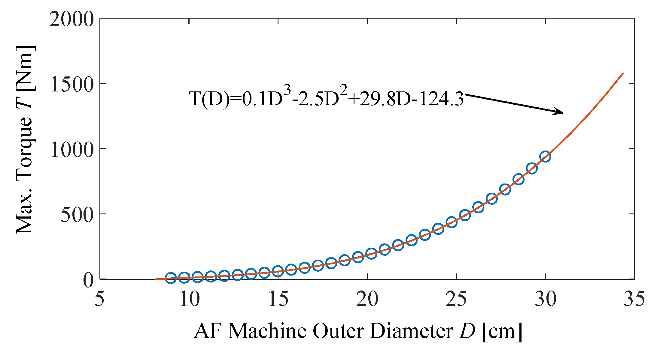
1.3. Advantages of Axial Flux Machines

As mentioned earlier, mid to high power yokeless AF machines have the potential to be more efficient and much smaller than the radial equivalents, as flux paths through stator can be shortened, decreasing magnetic losses and removing stator yoke. [7] In such truly three dimensional designs, the redundant mass not contributing to torque production or machine rigidity can be optimized in more ways, enabling further increases in the machine power density. The most important advantage of AF machines is their axially flat shape, ideal for mounting directly onto the driven device [4,7], combined with high torque density as electromagnetic force is applied at the high radius close to that of the whole electric machine, making them ideal for directly driven wind turbines, elevators, EVs [1] and enabling stacking of the machines on a single shaft to increase torque [4,10,11]. Axial Flux machines have great potential for use as EV wheel hub motors [4,6] when mechanical design challenges influencing durability are resolved.

To illustrate the influence of yokeless AF machine size on the electromagnetic torque (the same machine construction as described in the next sections), 3D Finite Element Analysis (FEA) results are plotted (Figure 1) as function of machine diameter $D$. The figure may be useful as a reference of the yokeless AF machine output torque trend while sizing an AF machine. Inner and outer diameter ratio were chosen to be $0.6$ for the machine, as it seems to be optimal for many designs [4].

It should be noted that the listed advantages of AF machines can be limited by many internal and external factors and compromises taken during the design process. For example, in higher diameter AF machines, it may be hard to provide adequate bearing and manufacturing precision to keep the air gap small [4].

2. Investigated Machines Models

2.1. Stator Construction

The chosen machine type was double air gap (two rotors with permanent magnet poles at each), single stator topology in which flux flows through the stator only axially and reverses in both rotors mounted anti-symmetrical to each other on the same shaft (Figure 2). Despite higher mass required by the rotors yokes, these constructions offer the highest efficiency by limiting losses in the stator. Furthermore, in practice, rotor yokes have to be thick enough to prevent resonance, which can play very significant role in some designs [12]. Additionally, to decrease redundant mass, the stator yoke was removed (yokeless); this AF machine type requires a more complicated mechanical design, which is not discussed in this paper.

To decrease the simulation time and simplify the design, the machines were composed of discrete stator cores each based on a trapezoid circumscribed with two inner and outer radii arcs. It is important to note that stator slots had symmetric sides as if they were drilled by a drill moving along the machine radius. This is one of the standard solutions maximizing stator core volume and providing a symmetric stator skewing-like effect, decreasing cogging torque. In a radial-flux machine, the stator cores or rotor poles would have to have trapezoidal intersections along a tangential plane to achieve a similar effect. The value of current density was chosen to represent well cooled AF machines.

No flux barriers representing laminations were added in the model because such stator cores would cause uneven flux densities at inner and outer radii, leading to magnetic saturation of the stator material at the inner radius (as visible at B field plot, Figure 3b). This design can be realized using, for instance, Soft Magnetic Composite materials (SMCs) as the stator core material [2].

To make the considered AF machines comparable, stator construction was invariant during simulations (

Table 1. Stator parameters.

Parameter	Value
Outer Diameter ($D_{out}$)	$300\mathrm{mm}$
Inner Diameter ($D_{in}$)	$180\mathrm{mm}$
Conductor Intersection Area	$480{\mathrm{mm}}^2$
Current Density (RMS)	20 $\frac{\mathrm{A}}{{\mathrm{mm}}^2}$

) and only certain rotor parameters were changed, as described in the next sections.

2.2. Rotor Construction

The rotor yoke was modeled as a solid disc with a hollow hole inside. The inner radius of the hollow space was smaller than that of the stator and of the rotor magnets’ inner edges. Such offset decreased flux density in the rotor yoke between poles by providing a wider flux path. Steel without any laminations was used as rotor yoke material. The poles were permanent magnets spanning along angle ${\sigma }_m$ described by the factor $\alpha$ and full pole span angle ${\sigma }_p$, depending on total number of poles $P$.

$${\sigma }_m=\alpha {\sigma }_p=\alpha \frac{2\pi }{P}$$

(1)

The pole magnets were SPM, as this construction offers higher torque and lower flux dissipation (Figure 3). The PM geometry can be further refined if i.e., lower back-emf distortion is needed by skewing its sides symmetrically [13] in a similar way as was described for the AF machine stator segments. The magnets might be later secured with retainer and resin, which would also reduce windage losses. Figure 3b presents the solved FEA model of one of the described constructions with flux density B field shown in color (some segments were hidden for better visualization).

Invariant parameters of the rotor (presented in

Table 2. Rotor parameters.

Parameter	Value
Rotor Yoke Thickness	8 $\mathrm{mm}$
Air Gap ($L_g$)	1 $\mathrm{mm}$
Magnet Thickness ($L_m$)	8 $\mathrm{mm}$

), as well as those of the stator, were chosen to be universal for all rotors and prevent saturation of the steel, thus it has to be noted that each construction can and should be further optimized to maximize power output and efficiency after a particular configuration has been chosen.

2.3. Windings Connection

The windings were two-layered and concentric, as AF machines’ small inner radius decreasing space between slots limits other possibilities, requiring longer end-windings. Only three-phase connections of the coils were considered.

The stator windings were connected differently depending on the rotor number of the poles.

Table 3. Phase windings connections for different pole numbers (symmetric half of 18 coils total). Each consecutive coil was numbered and assigned to appropriate phase (row); minus sign designates inverted connection.

Poles	Phase	Phase Coil #1	Phase Coil #2	Phase Coil #3
8	A	1	−3	5
	B	7	−9	2
	C	4	−6	8
12	A	1	4	7
	B	2	5	8
	C	3	6	9
14	A	1	−5	6
	B	2	−3	7
	C	−4	8	−9
16	A	−7	8	−9
	B	−1	2	−3
	C	−4	5	−6

presents a method of connecting coils for different numbers of rotor poles—for each pole number (left column), each of the coils numbered from 1 to 9 is written in the row corresponding to a phase group to which it is connected, while the minus sign denotes the inverse connection of terminals. The main principles guiding selection of the connections were maximization of back-emf amplitude and keeping the phase shift of each coil as close to $180°$ electrical as possible [14]. For some of the investigated machines, other configurations resulting in smaller magnitudes of back-emf are possible, which could offer some advantages, depending on the application, resulting in lower output torque.

2.4. Slots and Poles Configurations

Four different rotor pole numbers were investigated with the same stator as $N_s$ slots, each of the different poles per slots ratio $Q$, which is said to characterize back-emf and cogging torque of the whole group of the same ratio [8]. Therefore, the results can be interpreted as characterizing each the whole group.

Because the investigated yokeless AF machines had concentric windings and smallest cogging torque was desired, only fractional slot winding [14] (non-unity slots per pole per phase number) machines were modelled. In such machines, in general each rotor pole of the symmetric part of the machine is in a different position relative to its corresponding magnetic pole created by stator windings, thus smoothing out combined phase flux linkage when each phase’s coil flux linkages are superimposed. Consequently, back-emf waveforms, being the flux linkage derivatives, are smoothed out even more considerably by removing higher harmonics. The effect can be analyzed analytically [10,13,15], but in the case of the AF machines presented, it was more accurate to use 3D FEA.

The Greatest Common Divisor $GCD(P,N$_s), presented in

Table 4. Modeled rotor poles numbers.

P	Q	GCD(P, Ns)	Ns
8	0.44	2	18
12	0.67	6
14	0.78	2
16	0.89	2

, determines the smallest part of the machine that could be simulated (as the plane normal to the Y axis, marked with a line in Figure 2, in case of the model divided by 2). Each of the yokeless AF machines also had a symmetry plane normal to the shaft axis (or Z axis in Figure 2), which was used to cut the model in the middle by half—this allowed the simulation of only one rotor and half of the stator. By applying appropriate boundary conditions in finite element models and accounting for post-processing of the solutions by an appropriate factor, only the resulting smallest possible AF machines parts were solved to decrease computation time. Additionally, as $GCD(P,N$_s$)$ is equal to number of symmetries in the machine, it can also be used to predict parameters such as cogging torque in a fractional windings machine, therefore it was expected that the parameter would have significant influence on the results. For each different pole number $P$, the pole span $\alpha$ was stepped by $0.1$ from $0.4$ to $0.9$, yielding 6 different machine models with the same $P$.

2.5. Simulation Methods

In AF machines, magnetic flux distribution is often more complex than in regular radial flux machines and simplifications to 2D models of equivalent linear electric machines solved analytically or even with FEA cannot always provide accurate results. It is especially significant in AF machines without stator laminations, like the ones investigated in the paper, in which flux can flow radially from regions of higher potential. For this reason, 3D FEA was used and magnetic field distribution solved for each rotor position with the static solver. Resolution of the output data was 1 simulation step per $1°$ electrical, as further increases in resolution did not influence the results significantly.

As solving 3D finite element problem is much more time consuming, mesh was adjusted manually using sets of coefficients of parameterized mesh regions, edges and surfaces for each finite element model, to provide comparable results. A higher interpolation polynomial order was set for the regions with rapidly changing flux density distributions, such as air gap and aligning regions. Non-linear materials’ B–H curves were used to account for magnetic saturation [16].

Ideal electromagnetic torque in PM machines can be calculated independently of cogging torque only with two methods. One of the methods is to use a finite element model of an electric machine, with windings supplied with current, to calculate numerically total electromagnetic torque and then account for cogging torque, which has to be obtained from equivalent simulations of the open circuit machine. The other method is calculation of the ideal torque using only the open circuit FEA simulations, assuming sinusoidal or trapezoid current in the windings (as described in the next sections). The first method can be more accurate but requires more simulation steps. Due to the fact that 3D FEA simulations are time consuming and the results produced with both methods were not significantly different, the second method, based on calculations, was chosen.

After verifying that the finite element models with adjusted mesh produce negligible error, simulations and basic post-processing were run in batch on a computer cluster. The results were collected manually and processed further with the set of scripts to calculate additional quantities and plot the results.

3. Results of FEA Simulations

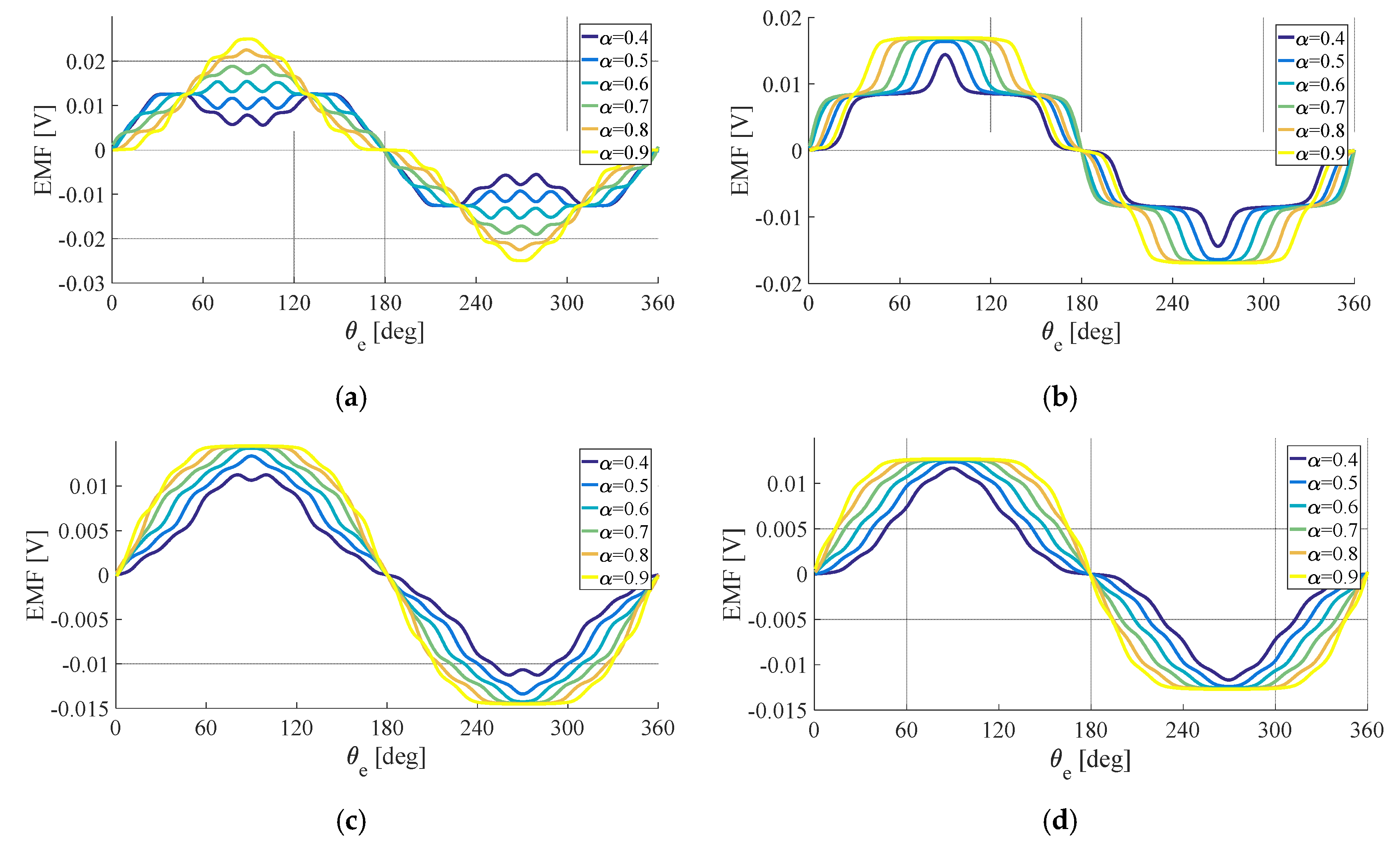
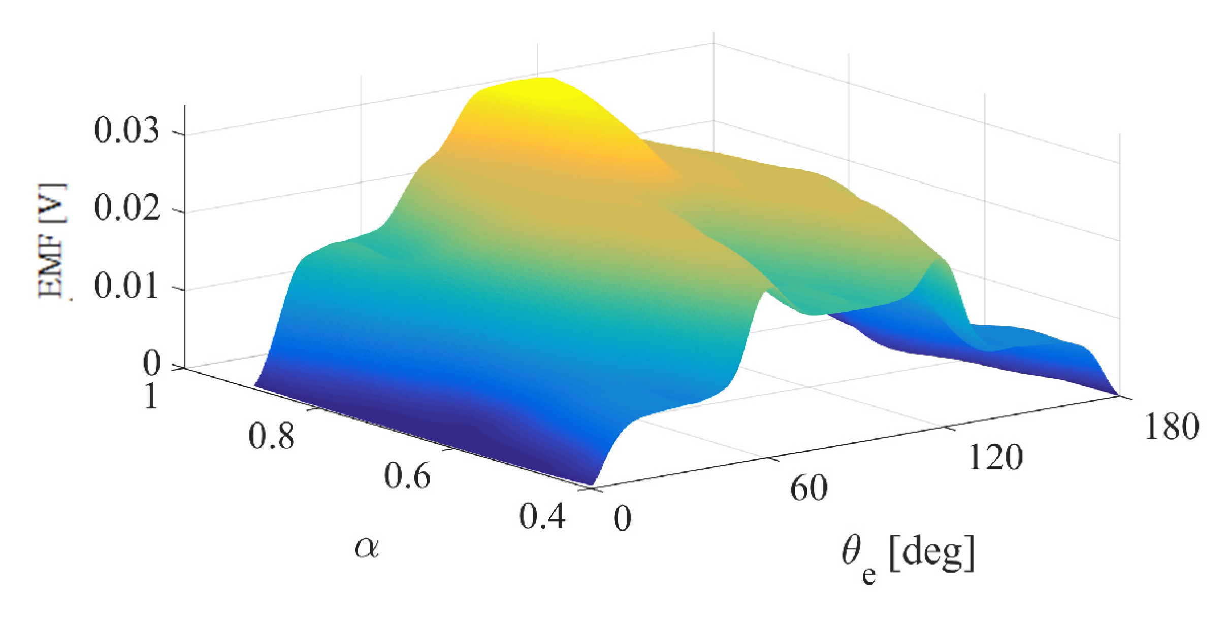
3.1. Back-Emf

The waveform of back-emf generated by the machine is one of the most insightful parameters calculated using FEA simulations data, as many other values such as ideal electromagnetic torque and power waveforms can be calculated on its base.

The data gathered from FEA simulation results were flux linkages $\lambda$ of each phase coil for sets of simulations steps with different rotor position angles expressed in electrical degrees ${\theta }_e$–from $0°$ to $90°$. Then, the back-emf $E$ was calculated using gathered flux linkages flowing through each of the modeled coils, adding them depending on the coils connection and then differentiating them with respect to rotor position angle. Flux linkages depend on the number of coil turns and flux through the coil $\varphi$, which can be written as $\lambda =\varphi N_c$. It can be observed that the data gathered from a set of static FEA simulations is dependent only on rotor position ${\theta }_e$, however, in reality, the angle must be dependent on time $t$ to calculate back-emf with Equation (2), therefore it follows that the results of flux linkage $\lambda$ differentiation with respect to the rotor position must be multiplied by some assumed electrical angular speed ${\omega }_e$.

$$E=\frac{d\lambda }{dt}=\frac{d\lambda }{d{\theta }_e\left(t\right)}\frac{d{\theta }_e\left(t\right)}{dt}=\frac{d\lambda }{d{\theta }_e} {\omega }_e=N_c\frac{d\varphi }{d{\theta }_e} {\omega }_e$$

(2)

The gathered back-emf waveforms correspond to rotation with an assumed ${\omega }_e=1\frac{rad}{s}$ electrical angular speed and one turn per coil ($N_c$), and can be interpreted as back-emf constant per one coil turn with units volts per angular speed per one coil turn per number of poles ($\mathrm{V}\cdot \mathrm{s}$). (Sometimes the unit of the constant is expressed as flux ($\varphi )$ in (Wb) when only the first harmonic approximation is considered, however it is not true for a real machine with non-perfect back-emf). This way, the presented waveforms can be scaled depending on the chosen number of coil turns and mechanical rotation angular speed. By designating the created measure as $k_{ee}$, it can be described with the Equation (3) and can be used to compare the results

$$k_{ee}=\frac{d\lambda }{d{\theta }_e}=\frac{d\lambda }{d{\theta }_m}p$$

(3)

where the ${\theta }_m$ is the mechanical rotor angle and $p=P/2$ is the number of pole pairs.

3.2. Phase Back-Emf Waveforms

The phase back-emf conveys the most information compared to the line emf as its distortion directly causes torque ripples. For this reason, the obtained results for each configuration are presented below as the first ones.

It can be observed that with increasing number of poles or decreasing number of slots per pole, the waveform is more smooth (Figure 4). Some of the configurations of the lower number of poles, and those with higher pole spans, seem to be useful for trapezoid BLDC drive having such flat tops. For this reason, they will be analyzed later using the introduced measure of $60°$ deviation from flatness.

3.3. Line Back-Emf Waveforms

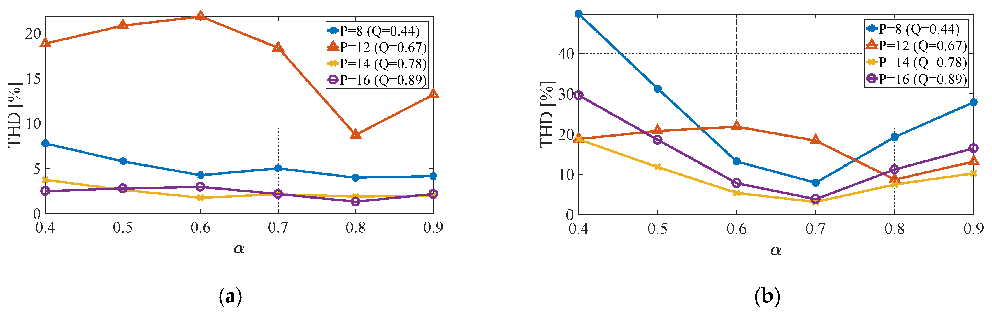
Observation of the back-emf between two lines phase is important in most cases as the star connection of electric machines is the most popular. The line back-emf is created simply by subtracting two phases of emf waveforms (one shifted by $120°$ three-phase system), and this operation acts as filtration, cancelling out harmonics, which are a multiplication of the number of phases. Thus, plots of line back-emf waveforms (Figure 5) convey less information, however, they are important to estimate voltage distortion in star connection.

Most waveforms are much smoother than that of phase back-emf. One significant configuration is that of 12 poles. It can be observed that difference in GCD of the configurations have great impact as the edges of poles and slots have more alignment points. The 12 pole configuration may be useful for the BLDC AF machine also in the star connection.

3.4. THD Comparison

Total Harmonic Distortion (THD) is a measure of how many, of all the harmonics except the signal frequency per amplitude of signal (in this case the fundamental), there are. It is useful to estimate how good the machine would perform as synchronous drive. The THD can be described as

$$THD=\frac{\left|A_s\right|}{\Sigma \left|A_i\right|}\cdot 100\%$$

(4)

The $\left|A_i\right|$ are amplitudes of all harmonics except the signal harmonics and $\left|A_s\right|$ is the amplitude of the signal. In this case, the signal is the fundamental frequency $\left|A_s\right|=\left|A_1\right|$, therefore $i\ne 1$.

By analyzing the phase back-emf with the THD measure (Figure 6), it can be confirmed that $P=12$ is in fact the characteristic configuration and all other configurations have minima around pole span $\alpha =0.7$. The $P=14$ and $P=16$ are the most suitable for synchronous drive as they have less harmonic distortion (around 3%).

In line back-emf, the trends are not so clearly visible and one easy to observe fact is that $P=12$ has far more distorted waveforms than the other one.

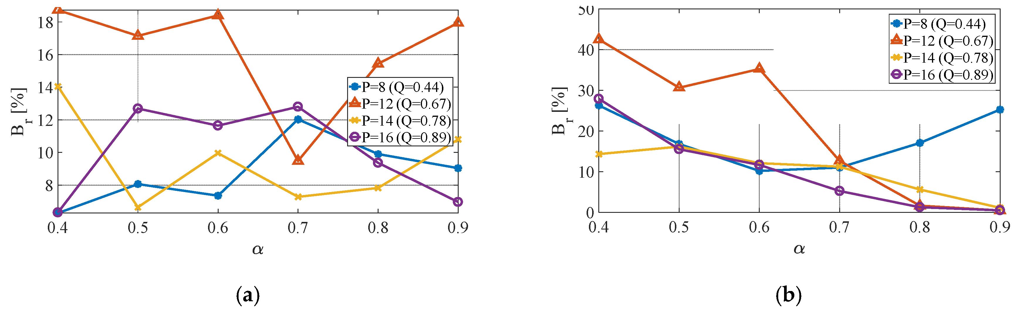
3.5. Trapezoid Ripple

To quantitatively estimate the fitness of the machine to be driven by trapezoidal voltage as BLDC drive, the measure of flatness at $60°$-$B_r$ is introduced.

$$B_r=\frac{\max \left(\left|{\overrightarrow{E}}_{60°}-mean\left({\overrightarrow{E}}_{60°}\right)\right|\right)}{mean\left(E_{60°}\right)}$$

(5)

where ${\overrightarrow{E}}_{60°}$ is the vector of back-emf of phase A from $60°$ to $120°$. Such a measure resulted in plots similar to THD, presented below (Figure 7).

The trends are clearly visible—the $P=12$ despite having different local minima, and the rest has decreasing $B_r$ with increasing pole span. The only odd configuration is the one with the least number of poles as it diverges to higher values at higher pole span coefficients.

Similarly to line THD analysis, the $B_r$ factor values of the line back-emf are also much more scattered and it is hard to see any trends. However, by observing the previously presented $P=12$ waveform, it can be stated that one minima not captured due to the resolution limited by simulation time would probably be between pole span coefficients $\alpha$ of 0.6 and 0.7. These values of $\alpha$ would probably be the most suitable for BLDC drive mode.

To present the existence of minima, a more clearly interpolated $P=12$ back-emf surface is presented in Figure 8 below.

3.6. RMS Comparison

Another important point of analysis it to observe the RMS values of the back-emf as they are closely related to the maximum torque and power magnitudes of the machine. These plots (Figure 9), as described earlier, are scaled by number of poles, therefore mainly the trends and maximum power (for different operating speeds ranges depending on number of poles) can be observed. The torque is calculated and analyzed later separately.

Both the line and phase back-emf magnitude slopes tend to decrease along with rising pole span, which is due to the magnetic saturation of the stator core.

3.7. Ideal Torque

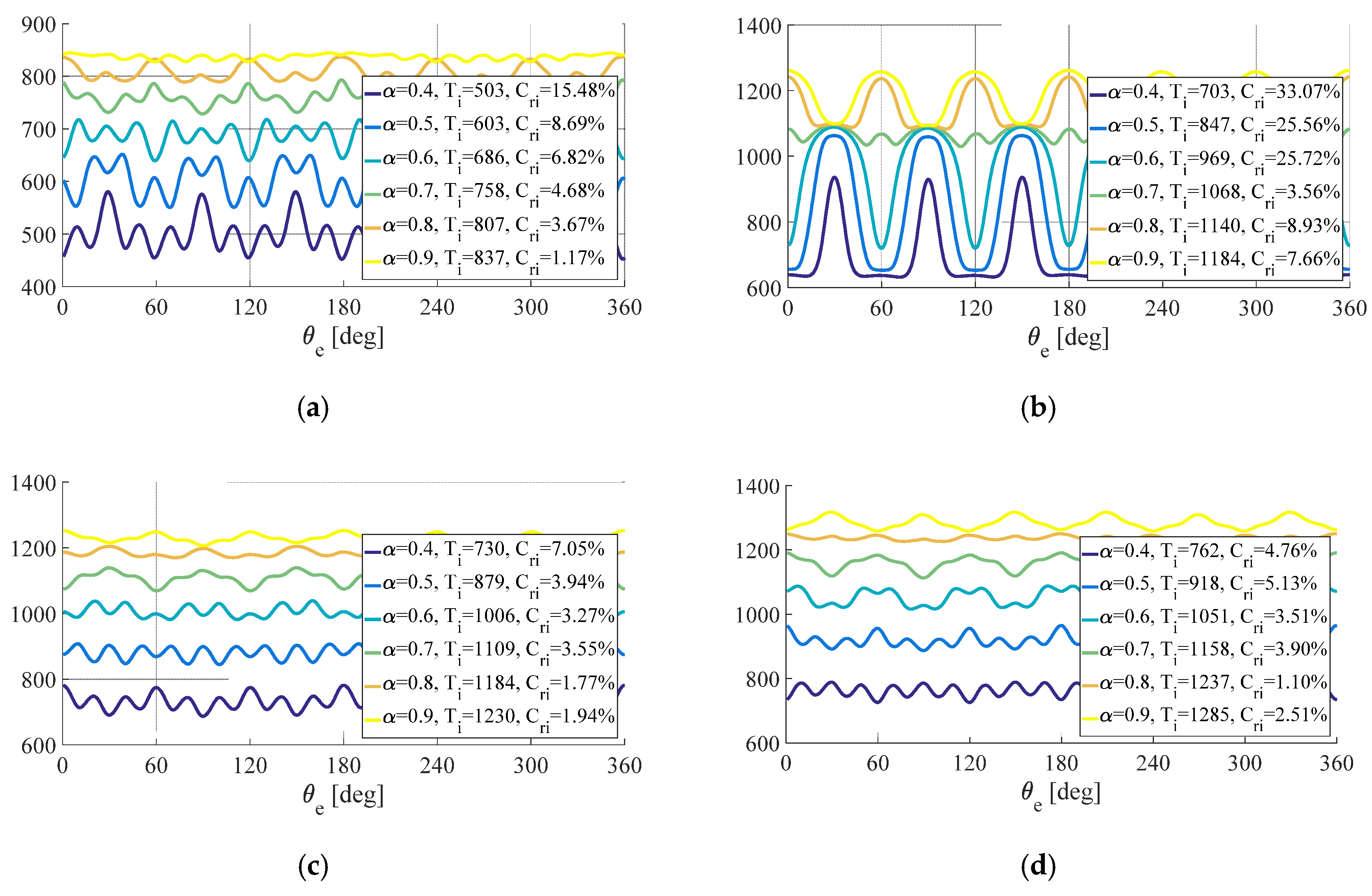
3.7.1. Ideal Torque Waveforms

Ideal torque $T_i$, the main component of total electromagnetic torque developed by the machine related to armature current interaction with magnetization field and PMs [11,15], can be calculated using FEA in two ways, as mentioned earlier. The simplest but not the most accurate way (neglecting stator slotting effect) is to simply compute ideal power $P_i$ using already calculated phase back-emf. This method allows independent calculation of the ideal torque component.

$$P_i=\mathsf{\Sigma } I\cdot E_{ph}$$

(6)

where I is the sinusoidal input armature current vector of one phase and $E_{ph}$ is the calculated vector of phase back-emf. The power of each phase, in this case 3, has to be summed as denoted in the Equation (6). To keep analyses simple, here, instead of ideal power $P_i$, the value of ideal torque $T_i$ was calculated, which in the case of this SPM machine is more useful, as it scales almost linear during operation (without filed-weakening) and its power depends on the chosen operating speed range, which is influenced by many factors such as resonance phenomena. Therefore, the ideal torque can be calculated as

$$T_i=\frac{P_i}{{\omega }_m}=\mathsf{\Sigma }I{k}_{ee}p$$

(7)

where the $k_{ee}$ is the scaled back-emf measure described earlier and $p$ is the number of pole pairs $p=P/2$. Using this relation, we can calculate ideal torque (Figure 10) using gathered static simulation data and the torque can be multiplied by ${\omega }_e$ to get the ideal power at any angular speed. It is important to note that this analysis holds for synchronous machines, and the factor $B_r$ considered earlier can be used to estimate the trapezoid driven BLDC machine.

The torque pulsations over one electrical revolution are clearly visible and can be further analyzed using other methods. The one odd configuration with mostly very high ripples is once again $P=12$.

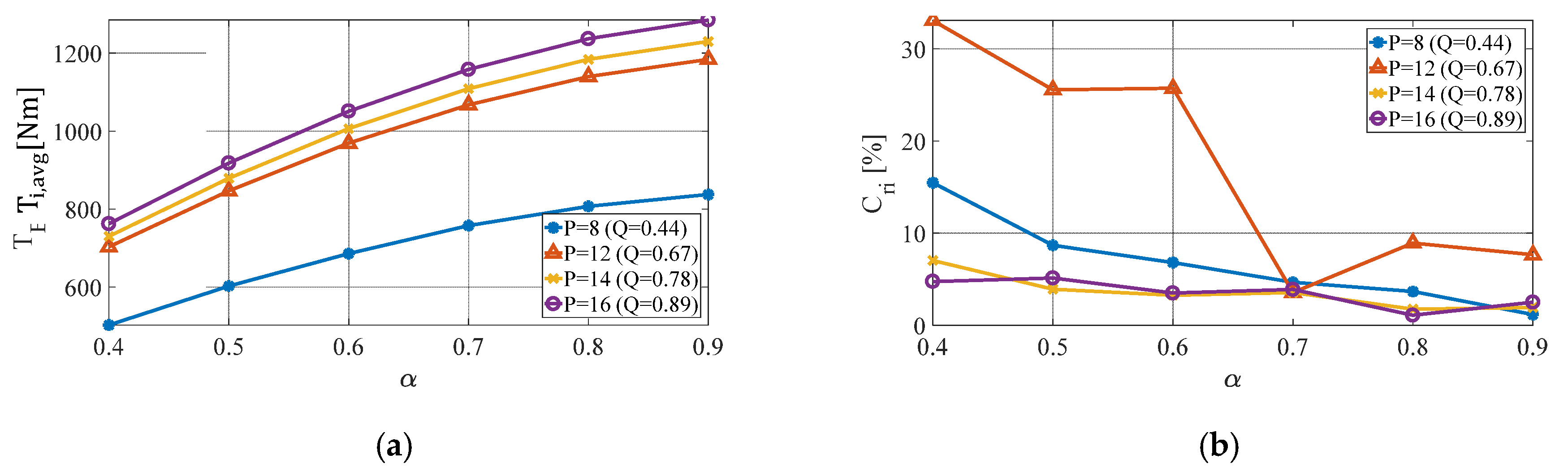
3.7.2. Ideal Torque Magnitudes & Ripples

To estimate actual usable machine torque, the data has to be averaged—below are presented results of that operation (Figure 11a). Visibly, the trends are similar to that of phase back-emf RMS values, however the order is changed because of use of back-emf scaled by number of poles. This fact does not discard the previous plot as the power of the machines would be similar after adjusting the machine operational speed—for example, $P=8$ would have much higher operational speed than the $P=16$ rotor.

3.7.3. Ideal Torque Ripple

Perhaps the most useful information, other than maximum torque and power, is the torque ripple factor named here $C_{ri}$ (Figure 11b). Moreover, the frequencies at which the torque pulses may be of the interest, as they can also cause resonance in mechanical parts, which was the case with the cogging torque.

The $C_{ri}$ factor presented here is defined in the same manner as described pulsation factor $B_r$, however instead of ${\overrightarrow{E}}_{60}$, the ideal torque waveforms presented in the previous section were used. The analysis is also valid only for synchronous drive mode.

From the plots presented, the optimum points for each variant of the machine supplied with sinusoidal current can be picked. The main trend is that the ripple factor decreases with increasing pole span $\alpha$.

3.8. Cogging Torque

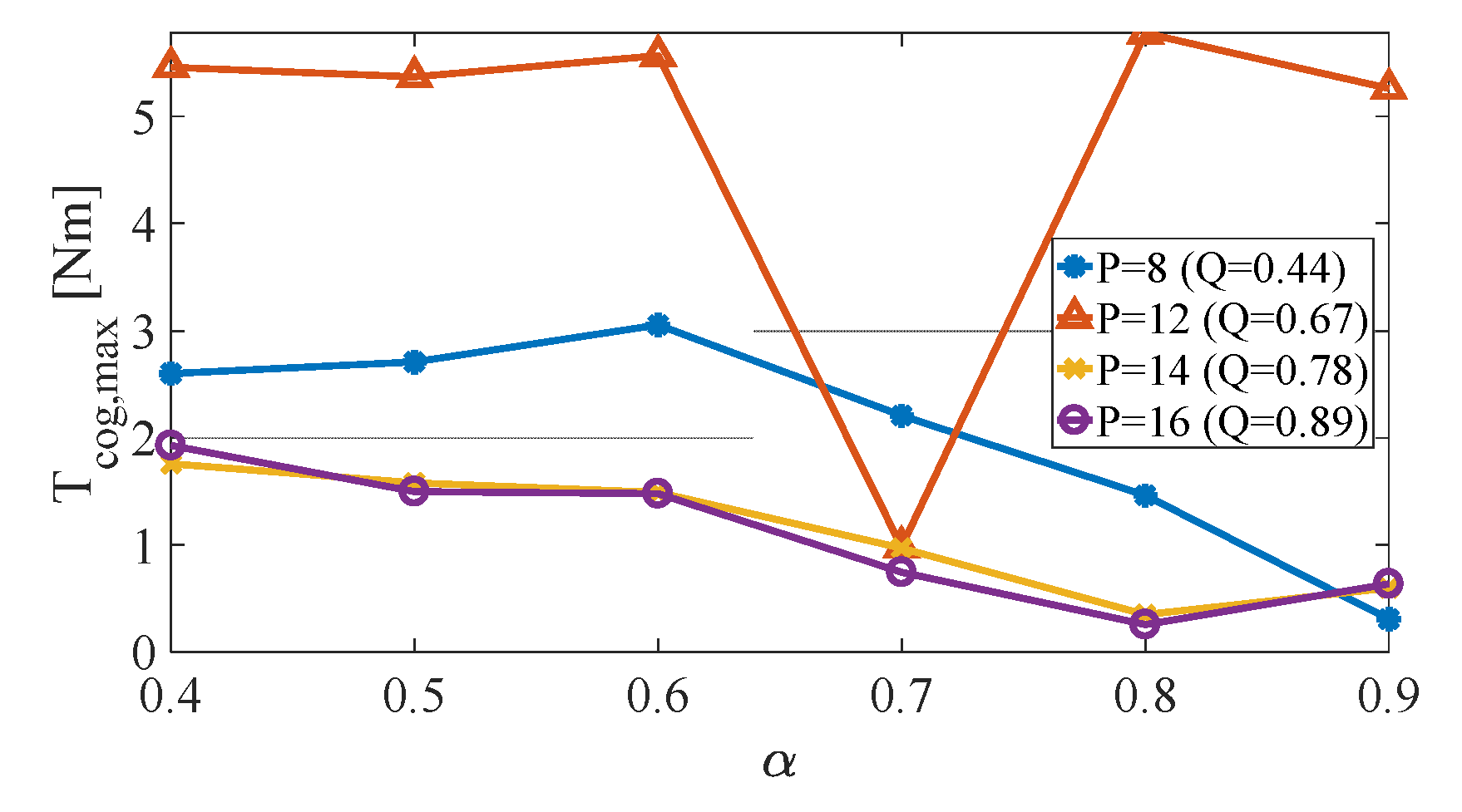
3.8.1. Maximum Cogging Torque Comparison

Cogging torque has a large impact on the final machine design, determines areas of applications suitable for the machine and may limit maximum speed (Figure 12). Permanent magnet motors exhibit constant cogging torque, in other words its magnitude is independent of machine speed or state. The influence of that torque will be greatest at low output torque operation.

The cogging torque is caused by magnets and teeth of the machine trying to align at the points of smallest total reluctance from magnet flux point of view. Therefore, the simplest way to minimize cogging torque is to minimize the number of points (positions of rotor) at which this happens. This relation also has influence on back-emf. To achieve that, the fractional pole pitch is chosen with the lowest GCD of number of slots and number of poles. Moreover, skewing of either stator or rotor can be employed to minimize this torque. However, this relationship is in practice not that simple, especially with three dimensional flux path, so the model was used to investigate it.

On the plot with the results, it can be seen that the cogging torque is rather low when compared to the ideal torque of each model. The machine with the highest count of alignment points ($P=12$) seems to exhibit the highest cogging torque, however it can be eliminated at pole span of ($\approx 0.7$). Other machine configuration cogging torques tend to decrease with increasing pole span coefficient.

It is important to remind that these AF machines have non-radial stator cores, which do not align with rotor magnets, which significantly decreases cogging torque.

3.8.2. Cogging Torque Spectra

Cogging torque as function of rotor position can be decomposed onto the harmonic frequencies to analyze frequency of possible mechanical resonances or mechanical vibrations which can significantly limit AF machine speed range. Such decomposition can be explained physically by occurrence of more than one set of equilibrium points at which stator and rotor want to align. Some of these configurations have higher and some lower alignment forces and when superimposed result in the measured net cogging torque of the electric machine. The harmonics are dependent upon slots and poles ratio and pole magnet span.

$$T_{cog}=T_{f1}+T_{f2}+\dots +T_{fn}$$

(8)

where $T_{cog}$ is cogging torque and $T_{fn}$ are components of it occurring at frequencies $f_{cog}=f_{\omega }n$, where $f_{\omega }$ is rotor mechanical revolutions frequency of the rotor and $f_{cog}$ is the mechanical frequency of $n$-th harmonic. Each of these $n$ harmonics can cause resonance phenomena in many mechanical parts, most importantly the rotor, because when it resonates and moves in the air gap, it can damage magnets and stator slots. In summary, it is important to decrease total magnitude of cogging torque and magnitude of these harmonics, which may cause resonance. For that purpose, the data below was used and compared with subsequent results of mechanical simulations.

The cogging torque shown (Figure 13) is plotted and analyzed as function of electrical degrees due to ease of processing, however, to use it in comparison with mechanical resonance frequency, it should be converted to function of mechanical degrees by simply scaling it by number of the machine poles. The presented cogging torque components frequencies $f_{cog}$ were scaled with mechanical rotor speed frequency $f_{\omega }$, which corresponds simply to the harmonic number $n$.

4. Summary

This work presented parameterized models of the yokeless Axial Flux machine with different rotor parameters. FEA simulations of the AF machine models, with different sets of constructional parameters, allowed comparison of their influence on back-emf, ideal and cogging torques. The investigated parameters were the number of poles with constant number of slots (four different constructions) and pole span (six different values), which resulted in analysis of 24 different AF machines. The chosen machine construction corresponds to the standard segmented and yokeless stator AF machine with dual air gap with slight modifications such as trapezoid base stator. The error of the FEA simulations was small and the resolution of rotation steps was high enough to provide accurate and reliable data. The simulation time was rather time consuming, therefore some of the minima were not covered by the chosen resolution of pole span and were approximated by use of interpolation. Overall, the presented results of the study provide a good overview of different machine configurations performance and can be used in the process of machine design or as reference in other research. Results of the simulations allowed conclusions regarding which AF machine configurations are more suitable for BLDC or synchronous drives and estimation of their performance.

Pole spans in the range of $0.7–0.8$ resulted in the smallest THD of phase back-emf waveforms for all numbers of poles. Analysis of line to line back-emf allowed identification of following THD minima: 3% at $P=14$ and $P=16$ with pole span $\alpha =0.4–0.9$, 8% at $P=8$ with $\alpha =0.7$ and 9% at $P=12$ with $\alpha =0.8$. Therefore, AF machines with 14 and 16 poles with a pole span close to 0.8 were the most suitable for synchronous drive in this regard, where pole span had a positive influence on the ideal torque developed. After interpolation of back-emf waveforms along varying pole span $\alpha$, it was concluded that the shape closest to trapezoid suitable for BLDC drive can be obtained with $P=12$.

Analysis of ideal electromagnetic torque waveforms obtained for sinusoidal current supply allowed calculation of torque ripple factors for all of the machine variants. The ideal torque ripple factor had a minima of 1.2% at $P=8$ with a pole span $\alpha =0.9$, 3.56% at $P=12$ with $\alpha =0.7$, 1.8% at $P=14$ with $\alpha =0.8$ and the lowest ripple of 1.1% at $P=16$ with $\alpha =0.8$. Therefore, the 16 pole AF machine seems to be the best for synchronous drive when disregarding increased frequency due to high number of poles. If high operating speed ranges are considered, the eight pole machine could be used with measures taken to minimize the THD, for instance, additional magnet skewing. However, higher pole configurations seem to be better in general, making the AF machine more suitable for low speeds.

Maximum values of cogging torque for constructions with numbers of poles of 8, 12, 14 and 16 are correspondingly 3, 8, 1.8, 2 Nm. Minimal cogging torque was obtained for pole spans in the range $\alpha =0.6–0.8$. For $P=8$, 12, 14 and 16, values of minima are 1.5, 1.0, 0.2 and 0.1 Nm. As mentioned earlier, such small cogging torque values are caused by slightly skewed construction of slots in relation to poles and by fractional values of slots per pole ratio Q.

Given cogging torque data along with the other results, it can be concluded that pole spans higher than 0.8 are not recommended and selecting value in between $0.7–0.8$ seem to be reasonable for synchronous drive, especially when PM size is to be minimalized due to their cost and durability.

5. Conclusions

Based on the on 3D FEA simulations results, it can be concluded that when the phase coils connections are chosen to maximize back-emf amplitude, the number of rotor poles has significant influence on the yokeless AF machine’s ideal and cogging torques amplitudes, averages, as well as their ripple factors. Pole numbers closer to the number of slots tend give better performance in such AF machines with concentric windings. The AF machines analyzed with higher poles are best suitable for low-speed operation, especially given their high electromagnetic torque with small ripple. As higher pole numbers result in higher frequencies at the same rotor speed, SMC materials can be used [13] as the stator core segments material to minimalize resulting magnetic losses. The pole span of around 0.8 of full pole pitch gives the best synchronous drive torque density with low torque ripple and low back-emf THD. In general, yokeless AF machines can be recommended for low-speed direct drive applications where high output torque density with low cogging are needed, such as larger EVs near-wheel direct drives or even wheel-hub drives when mechanical structure is made adequately durable and rigid.

References

1. Lampérth, M.U.; Malloy, A.C.; Mlot, A.; Cordner, M. Assessment of Axial Flux Motor Technology for Hybrid Assessment of Axial Flux Motor Technology for Hybrid. World Electr. Veh. J. 2015, 7, 187–194. [Google Scholar] [CrossRef] [Green Version]
2. Woolmer, T.; McCulloch, M. Analysis of the Yokeless And Segmented Armature Machine. In Proceedings of the 2007 IEEE International Electric Machines Drives Conference, Antalya, Turkey, 3–5 May 2007. [Google Scholar]
3. Gieras, J.F. Permanent Magnet Technology; CRC Press: Boca Raton, FL, USA, 2010. [Google Scholar]
4. Gieras, M.J. Axial Flux Permanent Magnet Brushless Machines; Springer: Dordrecht, The Netherlands, 2005. [Google Scholar]
5. Patel, A.N.; Suthar, B.N.; Panchal, T.H.; Patel, R.M. Comparative Performance Analysis of Radial Flux and Dual Air-Gap Axial Flux Permanent Magnet Brushless DC Motors for Electric Vehicle Application. In Proceedings of the 2018 2nd IEEE International Conference on Power Electronics, Intelligent Control and Energy Systems (ICPEICES), Delhi, India, 22–24 October 2018. [Google Scholar]
6. Profumo, F.; Zhang, Z.; Tenconi, A. Axial flux machines drives: A new viable solution for electric cars. In Proceedings of the 1996 IEEE IECON. 22nd International Conference on Industrial Electronics, Control, and Instrumentation, Taipei, Taiwan, 9 August 1996. [Google Scholar]
7. Tong, W. Mechanical Design of Electric Motors; CRC Press: Radford, VA, USA, 2014. [Google Scholar]
8. Hendershot, J.R. Brushless DC Motor Phase, Pole, and Slot Configuration; Magna Physics Corporation: Hillsboro, OH, USA, 1992. [Google Scholar]
9. Hendershot, J.R.; Miller, T.J.E. Design of Brushless Permanent-Magnet Motors; Magna Physics Publishing and Oxford University Press: Hillsboro, Ohio, USA, 1994. [Google Scholar]
10. Sitapati, K.; Krishnan, R. Performance comparisons of radial and axial field permanent magnet brushless machines. IEEE Trans. Ind. Appl. 2001, 37, 1219–1226. [Google Scholar] [CrossRef]
11. Hanselman, D. Brushless Permanent Magnet Motor Design; Magna Physics Publishing: Orono, ME, USA, 2006. [Google Scholar]
12. Parviainen, A. Design of Axial Flux Permanent-Magnet Low Speed Machines and Performance Comparison between Radial-Flux and Axial Flux Machines. Ph.D. Thesis, Lappeenranta University of Technology, Lappeenranta, Finland, 2005. [Google Scholar]
13. Kappatou, J.; Zalokostas, G.; Spyratos, D. 3-D FEM Analysis, Prototyping and Tests of an Axial Flux Permanent-Magnet Wind Generator. Energies 2017, 10, 1269. [Google Scholar] [CrossRef] [Green Version]
14. Pyrhönen, J.; Jokinen, T.; Hrabovcová, V. Design of Rotating Electrical Machines; Wiley: Chichester, UK, 2008. [Google Scholar]
15. Ostović, V. The Art and Science of Rotating Field Machines Design: A Practical Approach; Springer International Publishing: Cham, Switzerland, 2017. [Google Scholar]
16. Cardoso, J.R. Electromagnetics through the Finite Element Method; CRC Press: Boca Raton, FL, USA, 2016. [Google Scholar]
Figure 1. Maximum double air gap yokeless Axial Flux (AF) machine torque T as function of outer diameter D = D o u t with constant inner to outer diameter ratio of 0.6.
Energies 13 03418 g001
Figure 2. (a) Mapping of the AF machine on X’Z plane as linear machine as described in [11]. (b) Simplified yokeless stator cores shape illustration with parallel planes slots. The rotor had a shape based on two arcs with diameters D o u t and D i n .
Energies 13 03418 g002
Figure 3. (a) Single rotor pole magnet construction with slightly chamfered edges (8 poles AF machine). (b) Symmetric part of the modeled machine with some of the rotor yokes, magnets and stator cores hidden (16 poles AF machine)—magnetic flux density in tesla [T] plotted in color.
Energies 13 03418 g003
Figure 4. Phase back-emf of 8 poles (a), 12 poles (b), 14 poles (c) and 16 poles (d) rotors.
Energies 13 03418 g004
Figure 5. Line to line back-emf of 8 poles (a), 12 poles (b), 14 poles (c) and 16 poles (d) rotors.
Energies 13 03418 g005
Figure 6. Total Harmonic Distortion (THD) of line to line (a) and phase (b) back-emf.
Energies 13 03418 g006
Figure 7. Line to line (a) and phase (b) back-emf deviation from 60 ° trapezoid.
Energies 13 03418 g007
Figure 8. 12 poles line back-emf resampled surface.
Energies 13 03418 g008
Figure 9. Line to line (a) and phase (b) back-emf RMS values of different pole spans α .
Energies 13 03418 g009
Figure 10. Ideal electromagnetic torque T i in Nm of 8 poles (a), 12 poles (b), 14 poles (c) and 16 poles (d) rotors.
Energies 13 03418 g010
Figure 11. (a) Average ideal torque T i , a v g and (b) its ripple factor C r i for different pole spans α .
Energies 13 03418 g011
Figure 12. Cogging torque maximum (over rotor position) for different pole spans α .
Energies 13 03418 g012
Figure 13. Cogging torque spectrum of 8 poles (a), 12 poles (b), 14 poles (c) and 16 poles (d) rotors.
Energies 13 03418 g013