Abstract
The state feedback controller is increasingly applied in electrical drive systems due to robustness and good disturbance compensation, however its main drawback is related to complex and time consuming tuning process. It is particularly troublesome for designer, if the plant is compound, nonlinear elements are taken into account, measurement noise is considered, etc. In this paper the application of nature-inspired optimization algorithm to automatic tuning of state feedback speed controller (SFC) for two-mass system (TMS) is proposed. In order to obtain optimal coefficients of SFC, the Artificial Bee Colony algorithm (ABC) is used. The objective function is described and discussed in details. Comparison with analytical tuning method of SFC is also included. Additionally, the stability analysis for the control system, optimized using the ABC algorithm, is presented. Synthesis procedure of the controller is utilized in Matlab/Simulink from MathWorks. Next, obtained coefficients of the controller are examined on the laboratory stand, also with variable moment of inertia values, to indicate robustness of the controller with optimal coefficients.
1. Introduction
The electrical drive system with elastic joints occurs in many industrial machines like robot arms, conveyor belts, rolling-mill machines, and servo systems. A long shaft between the motor and load machine in mechanical part of the system provides very low resonant frequency [1,2]. Due to this, the motor speed differs to the load one, and speed oscillations may occur. Such behaviour of the machine can cause unsatisfactory product quality. Another problem with elastic joints is the coupling shaft stress, resulting in negative influence on a life-time of the machine mechanical part. For that reason, the elasticity of the shaft should be taken into account during synthesis of the control structure.
Many control methods have been developed to provide high-performance operation of the machinery, and to prevent the shaft stress and oscillations [3,4,5,6]. A considerable part of them is based on well-known proportional-integral-derivative (PID) controller due to its simple implementation, intuitive tuning methods and limitation of the physical variables. The complexity of considered plant causes that several modifications of PID control scheme have been proposed. These are based on additional reference signal filtering, introduction of additional feedback or modification of the controller structure [3,4,5,6]. As it was shown in [7], the state feedback speed controller provides satisfactory performance of the two-mass system. Recently, the SFC is getting significant attention by the researchers and it is applied in wide-range of applications, e.g., cascade-free permanent magnet synchronous motor (PMSM) speed control [8], dynamic voltage restorer [9], grid-connected inverter that operates under distorted grid [10], synchronization of doubly-fed induction generators [11]. It is caused by good disturbance compensation and cope with constraints [8]. On the other hand, the main drawback of the SFC is still related to the tuning process. Due to the lack of cascade control structure all coefficients of SFC have to be selected simultaneously. It should be pointed out that simultaneous selection of coefficients seems to be non-trivial task, especially for complex control system. There are two the most commonly used tuning methods: pole-placement technique and linear-quadratic regulator optimization (LQR) [12]. It is worth to point out that it is possible to force the system to have closed-loop poles at the desired locations, by choosing an appropriate gain matrix for state feedback controller. Then, the first approach requires to set closed-loop poles at desired location. The proper selection of poles location is mainly based on experience and expert knowledge in a field of control theory. Alternatively, to compute the state feedback control gain matrix in systematic way, the LQR can be used. This approach minimizes the performance index that takes into account the relative importance of respective state variables and the energy amount needed for control process. This importance is defined by user during selection of the weighting matrices Q and R. The initial guess of these matrices can be obtained with the help of Bryson’s method [13]. In this approach, initial values are selected using maximum value of states variables, what in most practical cases can be easily defined. As it was mentioned earlier, the Bryson’s method provides just an initial guess, therefore it requires an additional manual tuning. It can be concluded that both considered methods use the trial-and-error approach. For this reason the commonly used tuning procedures are very time-consuming and/or require an expert knowledge. Due to this researchers have taken into account the automatic tuning process. In [14], the auto-tuning of SFC for speed control of permanent-magnet synchronous hub motor (PMSHM) was proposed. In order to assure the optimal control, the Gray Wolf Optimization algorithm was employed to acquire the weighting matrices Q and R in linear-quadratic regulator optimization process. The authors proposed the complex fitness function with novel element, which is responsible for minimizing the overshoot of the step response. Comparison with different optimization algorithms, such as Particle Swarm Optimization and Genetic Algorithm, as well as with classical approach to speed control are also included. The obtained experimental results proved proper operation of proposed method. A similar approach to automatic selection of weighting matrices Q and R was proposed in [15] and [16]. The first article focuses on comparison of nature-inspired optimization algorithms, and three different fitness functions in speed control of PMSM, while the second one presents an auto-tuning method for state feedback voltage controller for DC-DC power converter. It is worth to point out that, the proposed approaches took into account the constraints of selected state and control variables of PMSM and DC-DC power converter, respectively. Both articles provide satisfactory step response thanks to SFC coefficients obtained from proposed tuning approach. The further research in this field is related to auto-tuning of SFC with constraints [17]. In this paper, the comparison of two constraint-handling methods applied in automatic tuning of SFC is included. The authors compare simple parameter-less Deb’s rules with augmented Lagrangian method. It is worth to pointing out that parallel implementation of auto-tuning methods is also taken into account in the research [18]. Due to commonly used in personal computers multi-core processors, parallelisation of time-consuming processes, e.g., constrained auto-tuning of SFC, is justified to reduce computation time. An application of new meta heuristic algorithm called Whale Optimization Algorithm for design of two-degree-of-freedom state feedback controller (2DOFSFC) for automatic generation control problem is presented in [19]. The Integral of Time multiplied Squared Error (ITSE), Integral of Time multiplied Absolute Error (ITAE), Integral of Squared Error (ISE), and Integral of Absolute Error (IAE) are taken into account during construction of the performance index required for controller design. The proposed automatic tuning method of 2DOFSFC provides stable and satisfactory operation of the interconnected power system, and better dynamic performances in terms of settling time, overshoot, and undershoot values in comparison to PI, PID and 2DOFPID controllers. In [20], design of state feedback and state feedback plus integral controllers for rotary inverted pendulum system have been presented. The optimal values of the state feedback controller were obtained by Particle Swarm Optimization algorithm. It was shown that optimized coefficients provide a better robustness and time response specifications in comparison to other controllers commonly applied for inverted pendulum system, i.e., fuzzy logic and fuzzy PD.
In this paper automatic tuning of SFC for two-mass system is presented. This paper includes entire process of auto-tuning procedure: (i) assumptions on desired step-response characteristics, (ii) definition of objective function based on the assumptions made and, (iii) application of nature-inspired optimization algorithm to optimize defined objective function. The ABC is applied to select optimal weighting matrices Q and R. The assumptions take into account practical aspects of the machinery operation i.e., the stress-free and chattering-free operation of the two-mass system. To present advantages of the proposed approach, comparison with analytically calculated coefficients is included. Additionally, the stability analysis for the control system, optimized using the ABC algorithm, is presented. Finally, robustness of the proposed control scheme is also investigated on the laboratory stand with elastic joint and variable moment of inertia.
The paper is organized as follows: Section 2 includes description of mathematical model of the plant, definition of the control law and analytical tuning method of the controller. The application of ABC for auto-tuning process, and objective function definition with respective discussion are included in Section 3. Section 4 contains simulation and experimental results of the proposed auto-tuning approach and the analytical one. Stability and dynamics analysis are also included in this section. Finally, conclusions are presented in the last section.
2. Mathematical Model of Control System
2.1. Model of the Two-Mass System
In order to design state feedback controller for speed control of the two-mass system, the state-space representation of mathematical model have to be introduced and it is specified by the following equation [21]:
with:
where: , and are the angular speed of the motor shaft, angular speed of the system output, and the reference signal of angular speed, respectively; is an electromagnetic torque generated by the motor; is the torsional torque; , and are mechanical time constants of the motor, the load and an elastic part, respectively. It should be noted that in this particular case all state variables are measurable. In order to ensure steady-state error-free operation for step changes of reference speed and load torque, the state-space variable has been introduced [22]. It is defined by the following equation:
It is worth to point out that control loop of electromagnetic torque (i.e., current loop) is usually modelled as first order system:
where: is equivalent current loop time constant. During synthesis of the regulator an ideal and immediate generation of electromagnetic torque was assumed. Therefore, dynamics of the current loop has been omitted, and . Such assumption is acceptable for relatively short time constant of the current control loop in comparison to the mechanical time constants, what occurs in this particular case. On the other hand, delays related to the electromagnetic torque excitation loop can be taken into account during design process of controller. In such a case Padè approximation can be applied, what will result in increasing of the model order. Finally, to simplify synthesis process of controller, the nonlinearities (i.e., friction torques of machines, backlash, etc.) were not considered. The time constants of TMS are listed in Table 1.

Table 1.
The two-mass system parameters.
2.2. State Feedback Controller
The control law for discrete state feedback controller suitable for implementation in microprocessor based drive obtained for (2) is defined as follows:
with:
where: n is a discrete time index; , , and are gain coefficients of SFC. In order to tune SFC, linear-quadratic optimization method (LQR) is employed. The choice is related to: (i) repeatable results of optimization, (ii) the lowest value of the performance index and, (iii) the best dynamical behaviour in comparison to pole placement technique and direct selection of coefficients [23]. A discrete performance index of LQR minimized during optimization procedure has the following form:
with:
where: , , , and are coefficients of penalty matrices. The block diagram of TMS with SFC is presented in Figure 1.

Figure 1.
Block diagram of two-mass system with state feedback speed controller.
2.3. Analytical Approach
For comparison purposes, coefficients of state feedback controller were also obtained using classical method. In this approach, a transfer function of the closed loop system shown in Figure 1 should be determined. It can be calculated from the following set of equations:
where:
Introducing the Laplace operator, above equations are presented below:
transforming this system of equations accordingly, the following equation is obtained:
based on above, the transfer function of closed control system can be defined:
Now, above expression and Equation (7), following transmittance can be calculated:
The characteristic equation is described by the following form:
In order to calculate the equations defining gains of state controller, the above equation should be compared to a reference equation (the same order). The following polynomial was assumed:
where: —resonant frequency, —damping coefficient. Comparing the elements with the same powers of the Laplace operator, the following system of equations is achieved:
and finally, after short transformations, the mathematical expressions are obtained:
3. Artificial Bee Colony Algorithm
The ABC was proposed by Karaboga in 2005 and it was inspired by intelligent foraging behaviour of honey bee swarm [24]. The ABC is global gradient-less optimization algorithm that provides better/similar performance than the most known algorithms (e.g., Differential Evolution, Particle Swarm Optimization, Genetic Algorithm) although it uses less control parameters and it can be efficiently used for solving multimodal and multidimensional optimization problems [25]. The task of bees is to find the position of food source with the highest nectar amount. Position of food source represents a possible solution of problem and nectar amount corresponds to the quality of the associated solution. Since the algorithm was inspired by foraging behaviour of honey bee swarm, it is divided into three phases:
- employed bees phase,
- onlooker bees phase,
- scout phase.
The algorithm sequentially executes depicted phases for predefined number of iterations (N). It is worth mentioning that single food source is connected to employed and onlooker bee, and the colony size () is the main parameter of the ABC. Each phase has determined task in optimization process. The employed bees phase corresponds for exploration of search-space. These bees look for another food source taking into account position from their memory and position of another randomly selected food source. Position of new food source is given by the following equation:
where: i is dimension index; , and are the new, actual and randomly selected food source, respectively. After evaluating the nectar amount value of new food source, it is compared with actual one. If new food source has higher amount of nectar, it replaces the actual food source. The onlooker bees phase corresponds to exploitation and bees during this phase use the additional information for generation of new food source position-nectar amount. Equation (16) is also used by the onlooker bees, but selection of random food source () is based on probability value, which is calculated as follows:
where: is selection probability of the food source (); is food source number; is the value of the objective function. It is worth to point out that modification rate parameter () is applied to optimization process. This parameter allows to reduce diversity of the colony during onlooker bees phase and it does not effect the exploitation. The pseudocode of ABC is presented in Algorithm 1.
| Algorithm 1 Artificial Bee Colony algorithm. |
|
The parameters of ABC used in auto-tuning process of SFC for TMS are summarized in Table 2, and these were selected according to information presented in [15]. It should be noted that chosen ABC parameters provides good exploitation and fast convergence in the global minimum.
Table 2.
Artificial Bee Colony parameters.
Objective Function
As it was mentioned earlier, TMS is a complex mechanical device where the load angular speed differs from the motor one and where speed oscillations may occur. Due to this tuning process of controller seems not to be trivial task, especially if non-cascade structure is used. In order to apply tuning procedure based on the above-mentioned ABC algorithm, requirements related to the desired step-response characteristics should be defined. These are as follows:
- overshoot-free response,
- rise and settling times as short as possible,
- chattering-free control signal,
- limited noise amplification.
In order to assure above-mentioned requirements during auto-tuning process, complex objective function is required. Its respective components will be responsible for fulfilment of depicted above requirements. Firstly, to minimize rise and settling times, the error of angular speed of the system output () needs to be minimized. Next, to reduce fluctuation of tension in elastic part and to assure overshoot-free step-response of TMS, the objective function is extended by component with derivative of difference between velocity before () and after () elastic part. The last elements from list depicted above are chattering-free control signal and limited noise amplification. In order to fulfill these requirements, a punishment for control signal changes has been introduced to the objective function. Finally, according to information presented in [26], time and error of angular speed of the system output () were introduced to the objective function as squared ones to reduce the overshoot and oscillations. The summarized objective function has following form:
with:
where: T is the test duration; and are manually selected coefficients. It is worth to point out that value of parameter is inverse proportional to fluctuation of tension in elastic part of TMS while the parameter corresponds for limit of noise amplification. The parameters have been chosen by trial-and-error approach to achieve desired step-response characteristics and allowable tension in elastic part.
4. Experimental Results
4.1. Simulation Case
The proposed auto-tuning method was implemented in Matlab/Simulink environment and the optimization last for 8 min using Acer laptop with i7-6700HQ supported by 8 GB RAM. According to information depicted in Section 2, an ideal electromagnetic torque shaping loop was established, which does not introduce additional delays. As it was mentioned earlier, proposed auto-tuning method was compared with analytical approach depicted in Section 2.3. Chosen values of design parameters are as follows: , . It is worth to point out that the damping factor and the resonance frequency were manually selected to achieve similar rise time () for both considered approaches, i.e., auto-tuning and analytical.
The objective function in iteration domain is presented in Figure 2. Values of the objective function for coefficients of SFC obtained by ABC algorithm and calculated analytically are equal to and , respectively. Values of Q and R matrices obtained for ABC algorithm are summarized in Table 3, while SFC coefficients for both considered approaches (i.e., supported by ABC optimization and calculated analytically) are listed in Table 4. The angular speed of the motor shaft and the system output, electromagnetic torque generated by the motor, and torsional torque step response obtained for both methods are presented in Figure 3. Table 5 summarizes selected step-response indicators, and one can see that difference of rise times is negligible small. The settling time () is shorter for analytical method, while the overshot () is smaller for the proposed approach. The disturbance compensation is similar for both sets of coefficients. The main difference between step responses, for analytical and the proposed method, is visible in electromagnetic torque waveform. The proposed approach provides smoother control signal in comparison to the analytical one, what was expected due to smaller values of controller coefficients. On the other hand, the dynamic and disturbance compensation for both sets of coefficients are comparable.
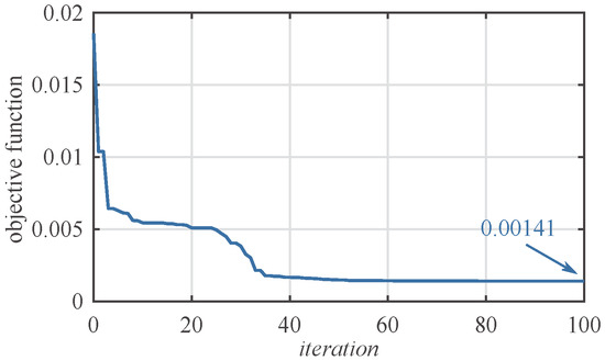
Figure 2.
Objective function in iteration domain.
Table 3.
Values of Q and R matrices obtained for ABC algorithm.
Table 4.
Comparison of coefficients of SFC obtained by the ABC algorithm and calculated analytically (calc).

Figure 3.
Step response for coefficients of SFC: (a) obtained for the ABC algorithm; (b) calculated analytically. From top: angular speed of the motor’s shaft and the system output, electromagnetic torque generated by the motor and torsional torque (simulation case).
Table 5.
Values of step-response indicators obtained for both considered methods for step change of reference signal (simulation case).
It is worth to point out the obtained coefficients of SFC by ABC are noticeable smaller than the analytically calculated coefficients, while the dynamical properties and disturbance compensation are similar for both sets of coefficients. As it was shown in [23], it is related to application of LQR in auto-tuning process, where control effort is taken into account during synthesis process of controller.
4.2. Dynamic Properties Analysis
Precision, fast response and stability are the most important features of control systems. This issues take significant part of work presented in control theory, and are important for industrial applications. In this article state feedback controller with constant parameters is considered. Moreover, nonlinear elements are neglected. Thus, it can be treated as a time-invariant system. In contrast to, for example, adaptive control systems (e.g., neural adaptive structures), where the most often used methods (for stability analysis) are based on Lyapunov’s theorems, in this case analysis of poles seems to be useful.
For described control structure, dependence of dynamic properties and position of poles, was analyzed. Results are presented in Figure 4, Figure 5 and Figure 6. System has four poles (two of them have equal real parts). Independent placement of those values can be achieved using modified reference Equation (13). Firstly, constant damping factor was assumed. Higher values of resonant frequency move the poles to the left side of S-plane (Figure 4). With this tendency, shorter rise time and better reaction against load switching can be observed. Decreasing the factor causes increase in oscillations (Figure 5). It is significant phenomenon during design of control method for two-mass system (elastic shaft leads to disturbances observed in state variables). Using the classical tuning method of the state controller, the poles are arranged by parameters and . In this case, using the ABC method, the position of the poles can be forced using other definition of cost function or changing the waveform of reference signal. Next test presents analysis for speed control system with parameters optimized using the ABC algorithm (Figure 6). Four poles are observed, each pair has the same imaginary part. All poles have negative real part, thus it can be assumed as the stability proof for the control system. Additionally high dynamics and precision of control should be noted.
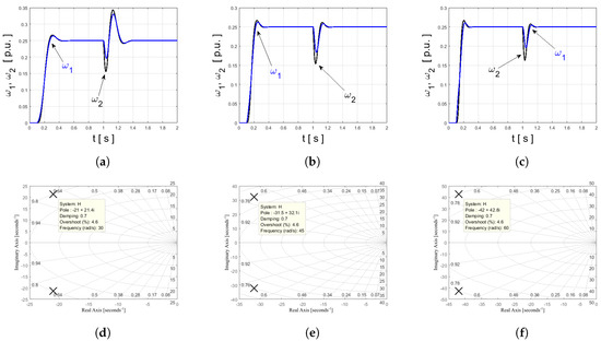
Figure 4.
An influence of locus position on dynamics of transients: (a,d) and = 0.7; (b,e) and = 0.7; (c,f) and = 0.7.

Figure 5.
An influence of locus position on dynamics of transients: (a,d) and = 1; (b,e) and = 0.7; (c,f) and = 0.5.
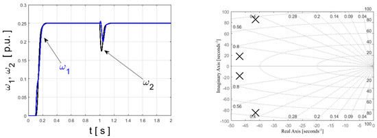
Figure 6.
Root locus plot of the speed control structure—results for ABC-auto-tuning method.
4.3. Experimental Examination
Presented in previous sections theoretical considerations were verified on a laboratory stand. The experiment was prepared for a drive presented in Figure 7. The system consists of a two DC motors mechanically coupled using elastic connection (about m length, 5 mm diameter, material: steel). The nominal power of both machines was kW. The motors operate under speed control structure, with state space controller, based on cascade control strategy. For part of the calculations, related to the electromagnetic torque, threshold of sampling time was used ( = 0.1 ms). The second part of algorithm implementation (speed controller) was done with t = 1 ms. It was assumed in order to influence of measurement noise reduction. The incremental encoders, attached to rotor of motors, generate signal (36,000 pulses per rotation) for speed calculation. The ADC converter reads information from current transducer, then processed to torque transient. The data collection, control algorithm and generation of control signals for power electronic devices (H-bridge) are processed in system for rapid prototyping based on dSPACE 1103 card. ControlDesk was used as a virtual control panel (parameters of control structure settings, data managing, preview of transients, etc.).
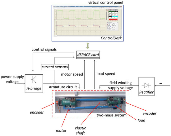
Figure 7.
Topology of the drive used in experiment.
Experimental step response for both considered sets of coefficients are shown in Figure 8, while step-response indicators are presented in Table 6. From obtained experimental results one can see that the analytically calculated coefficients dangerously amplify measurement noise. Due to this the torque load was not applied during experiment for safety reasons. It is worth pointing out that step-response indicators in simulations and experiments are similar. Coefficients obtained by the proposed auto-tuning process provide shorter rise time in experiments than analytical ones. The settling time value is higher for ABC coefficients than for calculated ones, what is consistent with simulation. The overshoot values in experimental case are the same for both sets of coefficients, and it is caused by the measurement noise. Although step responses for simulation and experimental cases slightly differs, the overall behavior as well as indicators are similar. Observed difference is mainly related to simplified model of plant used in synthesis process of SFC, where nonlinearities (e.g., friction components) and elasticities were omitted. As in a case of simulation study, control signal for automatically obtained SFC is smoother and the noise amplification does not occur, while the dynamic properties are comparable.
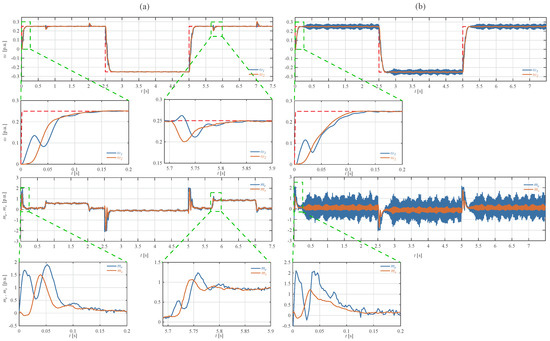
Figure 8.
Step response for coefficients of SFC: (a) obtained by the ABC algorithm; (b) calculated analytically. From top: angular speed of the motor’s shaft and the system output, electromagnetic torque generated by the motor and torsional torque (experimental case).
Table 6.
Values of step-response indicators obtained by the ABC algorithm and calculated analytically (calc) for step change of reference signal (experimental case).
Finally, the additional experiment with increased moment of inertia was made to investigate robustness of the automatically determined controller coefficients. It should be noted that moment of inertia was doubled on the laboratory stand. Recorded waveforms are presented in Figure 9, while selected step-response indicators are as follows: s, s and %. One can see that the rise time does not change, while the settling time and overshoot increased noticeably. Despite this, the step response is acceptable even for doubled moment of inertia value, what indicates robustness of automatically tuned controller.
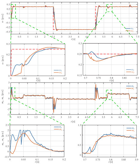
Figure 9.
Step response for coefficients of SFC obtained by the ABC algorithm–additional moment of inertia element in mechanical part in the laboratory stand. From top: angular speed of the motor’s shaft and the system output, electromagnetic torque generated by the motor and torsional torque (experimental case).
5. Conclusions
This paper presents an alternative design method applied for an electrical drive with a complex mechanical part. For this purpose a metaheuristic algorithm–Artificial Bee Colony–was applied. Special application, combining the main assumptions of the ABC and analyzed plant, was performed. The two-level structure of implementation allows easy (possible) modification of the plant parameters and configuration. Changes of parameters, nonlinearities and measurement noise can be considered during design process. Effectiveness of proposed method has been demonstrated in simulation and experimental studies. Theoretical analysis shows stable work of the control structure.
The entire controller synthesis process is described in details. The objective function components have been deeply discussed with particular emphasis on requirements related to desired step-response characteristics of complex two-mass mechanical system.
In order to show benefits of proposed approach, the analytical one was also taken into account. It was found that coefficients of SFC obtained by proposed automatic approach provides similar dynamic performance in comparison to coefficients calculated analytically, while these are noticeable smaller. The experimental examination proves that the coefficients obtained by the analytical method dangerously amplify measurement noise and provide undesirable chattering of control signal. For that reason, the proposed auto-tuning process seems to be more proper to achieve high-performance control of TMS and its safety operation.
The robustness of obtained coefficients of SFC has been examined in additional test with increased moment of inertia. Although the overshoot is observed in step response with additional moment of inertia, the overall dynamic properties are acceptable. It is worth to point out that two times higher value of inertia is usually applied for experimental evaluation of more complex control schemes, such as adaptive and iterative one. Therefore, results obtained for the proposed approach (where constant structure of controller is considered), are satisfactory and indicates its robustness.
The proposed automatic tuning method may be applied in commercial electrical drive system with elastic joints. This approach allows to reduce speed oscillations caused by difference between the the motor speed and the load one. It is worth to point out that the proposed method takes into account limitation of noise amplification. Due to above mentioned properties, the proposed auto-tuning method may find application in many industrial machines like conveyor belts, servo systems, robot arms and rolling-mill machines. It provides satisfactory product quality and extend life-time of the machine mechanical part due to reduced the coupling shaft stress.
Author Contributions
Conceptualization, R.S. and T.T.; methodology, R.S. and T.T.; software, R.S. and M.K.; validation, R.S., T.T. and M.K.; formal analysis, T.T.; investigation, M.K. and R.S.; resources, M.K.; data curation, R.S.; writing—original draft preparation, R.S. and M.K.; writing—review and editing, T.T. and M.K.; visualization, R.S.; supervision, T.T.; project administration, T.T.; funding acquisition, T.T. All authors have read and agreed to the published version of the manuscript.
Funding
This research was supported by the “Excellence Initiative—Research University” programme of Nicolaus Copernicus University, Poland and the basic research fund of Department of Electrical Machines, Drives and Measurements, Wroclaw University of Science and Technology, Poland.
Conflicts of Interest
The authors declare no conflict of interest.
References
- Szabat, K.; Wróbel, K.; Dróżdz, K.; Janiszewski, D.; Pajchorwski, T.; Wójcik, A. A fuzzy unscented Kalman filter in the adaptive control system of a drive system with a flexible joint. Energies 2020, 13, 2056. [Google Scholar] [CrossRef]
- Kamiński, M.; Orlowska-Kowalska, T. Adaptive neural speed controllers applied for a drive system with an elastic mechanical coupling—A comparative study. Eng. Appl. Artif. Intell. 2015, 45, 152–167. [Google Scholar] [CrossRef]
- Szabat, K.; Orlowska-Kowalska, T. Vibration suppression in a two-mass drive system using PI speed controller and additional feedbacks—Comparative study. IEEE Trans. Ind. Electron. 2007, 54, 1193–1206. [Google Scholar] [CrossRef]
- Ma, C.; Cao, J.; Qiao, Y. Polynomial-method-based design of low-order controllers for two-mass systems. IEEE Trans. Ind. Electron. 2012, 60, 969–978. [Google Scholar] [CrossRef]
- Serkies, P.J.; Szabat, K. Application of the MPC to the position control of the two-mass drive system. IEEE Trans. Ind. Electron. 2012, 60, 3679–3688. [Google Scholar] [CrossRef]
- Saarakkala, S.E.; Hinkkanen, M.; Zenger, K. Speed control of two-mass mechanical loads in electric drives. In Proceedings of the 2012 IEEE Energy Conversion Congress and Exposition (ECCE), Raleigh, NC, USA, 15–20 September 2012; pp. 1246–1253. [Google Scholar]
- Szabat, K.; Orlowska-Kowalska, T. Adaptive control of the electrical drives with the elastic coupling using Kalman filter. Adapt. Control 2009, 4, 205–226. [Google Scholar]
- Tarczewski, T.; Skiwski, M.; Niewiara, L.; Grzesiak, L. High-performance PMSM servo-drive with constrained state feedback position controller. Bull. Pol. Acad. Sci. Tech. Sci. 2018, 66, 49–58. [Google Scholar]
- Roldán-Pérez, J.; García-Cerrada, A.; Rodríguez-Cabero, A.; Zamora-Macho, J.L. Comprehensive Design and Analysis of a State-Feedback Controller for a Dynamic Voltage Restorer. Energies 2018, 11, 1972. [Google Scholar] [CrossRef]
- Bimarta, R.; Tran, T.V.; Kim, K.H. Frequency-adaptive current controller design based on LQR state feedback control for a grid-connected inverter under distorted grid. Energies 2018, 11, 2674. [Google Scholar] [CrossRef]
- Abo-Khalil, A.G.; Alghamdi, A.S.; Eltamaly, A.M.; Al-Saud, M.; RP, P.; Sayed, K.; Bindu, G.; Tlili, I. Design of State Feedback Current Controller for Fast Synchronization of DFIG in Wind Power Generation Systems. Energies 2019, 12, 2427. [Google Scholar] [CrossRef]
- Ogata, K.; Yang, Y. Modern Control Engineering; Prentice Hall: Upper Saddle River, NJ, USA, 2010; Volume 5. [Google Scholar]
- Franklin, G.F.; Powell, J.D.; Workman, M.L. Digital Control of Dynamic Systems; Addison-Wesley: Menlo Park, CA, USA, 1998. [Google Scholar]
- Sun, X.; Hu, C.; Lei, G.; Guo, Y.; Zhu, J. State feedback control for a PM hub motor based on gray wolf optimization algorithm. IEEE Trans. Power Electron. 2019, 35, 1136–1146. [Google Scholar] [CrossRef]
- Tarczewski, T.; Grzesiak, L.M. An application of novel nature-inspired optimization algorithms to auto-tuning state feedback speed controller for PMSM. IEEE Trans. Ind. Appl. 2018, 54, 2913–2925. [Google Scholar] [CrossRef]
- Tarczewski, T.; Niewiara, Ł.J.; Grzesiak, L.M. Application of artificial bee colony algorithm to auto-tuning of state feedback controller for DC-DC power converter. Power Electron. Drives 2016, 1, 83–96. [Google Scholar]
- Szczepanski, R.; Tarczewski, T.; Erwinski, K.; Grzesiak, L.M. Comparison of Constraint-handling Techniques Used in Artificial Bee Colony Algorithm for Auto-Tuning of State Feedback Speed Controller for PMSM. In Proceedings of the 15th International Conference on Informatics in Control, Automation and Robotics (ICINCO 2018), Porto, Portugal, 29–31 July 2018; Volume 1, pp. 279–286. [Google Scholar]
- Szczepanski, R.; Tarczewski, T.; Grzesiak, L.M. Parallel computing applied to auto-tuning of state feedback speed controller for PMSM drive. In ITM Web of Conferences; EDP Sciences: Les Ulis, France, 2019; Volume 28, p. 01031. [Google Scholar]
- Simhadri, K.S.; Mohanty, B.; Panda, S.K. Comparative performance analysis of 2DOF state feedback controller for automatic generation control using whale optimization algorithm. Optim. Control Appl. Methods 2019, 40, 24–42. [Google Scholar] [CrossRef]
- Ali, H.I.; Naji, R.M. Optimal and robust tuning of state feedback controller for rotary inverted pendulum. Eng. Technol. J. 2016, 34, 2924–2939. [Google Scholar]
- Kamiński, M. Zastosowanie algorytmu BAT w optymalizacji obliczeń adaptacyjnego regulatora stanu układu dwumasowego. Przegląd Elektrotechniczny 2017, 93, 300–304. [Google Scholar] [CrossRef]
- Franklin, G.F.; Powell, J.D.; Emami-Naeini, A.; Sanjay, H. Feedback Control of Dynamic Systems; Pearson: London, UK, 2015. [Google Scholar]
- Tarczewski, T.; Niewiara, L.; Grzesiak, L. Artificial bee colony based state feedback position controller for PMSM servo-drive—The efficiency analysis. Bull. Pol. Acad. Sci. Tech. Sci. 2020. early access article. [Google Scholar]
- Karaboga, D. An Idea Based on Honey Bee Swarm for Numerical Optimization; Technical Report; Erciyes University: Kayseri, Turkey, 2005. [Google Scholar]
- Karaboga, D.; Akay, B. A comparative study of artificial bee colony algorithm. Appl. Math. Comput. 2009, 214, 108–132. [Google Scholar] [CrossRef]
- Basquel, P.; Burke, R.; Curran, P. Optimal closed-loop transfer functions for non-standard performance indices. In Proceedings of the 2017 28th Irish Signals and Systems Conference (ISSC), Killarney, Ireland, 20–21 June 2017; pp. 1–6. [Google Scholar]


© 2020 by the authors. Licensee MDPI, Basel, Switzerland. This article is an open access article distributed under the terms and conditions of the Creative Commons Attribution (CC BY) license (http://creativecommons.org/licenses/by/4.0/).