How the Italian Residential Sector Could Contribute to Load Flexibility in Demand Response Activities: A Methodology for Residential Clustering and Developing a Flexibility Strategy

Abstract

This work aims at exploring the potential contribution of the Italian residential sector in implementing load flexibility for Demand Response activities. In detail, by combining experimental and statistical approaches, a method to estimate the load profile of a dwelling cluster of 751 units has been presented. To do so, 14 dwelling archetypes have been defined and the algorithm to categorise the sample units has been built. Then, once the potential flexible loads for each archetype have been evaluated, a control strategy for applying load time shifting has been implemented. That strategy accounts for both the power demand profile and the hourly electricity price. Specifically, it has been assumed that end users access a pricing mechanism following the hourly trend of electricity economic value, which is traded day by day in the Italian spot market, instead of the current Time of Use (TOU) system. In such a way, it is possible to flatten the dwellings cluster profile, limiting undesired and unexpected results on the balancing market. In the end, monthly and yearly flexibility indexes have been defined along with the strategy effectiveness parameter. From calculations, it emerges that a dwelling cluster for the Italian residential sector is characterised by a flexibility index of 10.3% and by a strategy effectiveness equal to 34%. It is noteworthy that the highest values for flexibility purpose have been registered over the heating season (winter) for the weekends.

1. Introduction

The European Union established the ambitious net zero greenhouse gas emissions target by 2050. Actions heading towards the energy systems decarbonisation can be implemented by the application of energy efficiency measures and by increasing Renewable Energy Sources (RES) penetration [1]. However, large-scale RES integration within electrical systems shows important technical and safety issues, due to the RES non-programmable nature. As a consequence, figuring out, effectively, the energy supply and demand matching will play a key role in the near future [2]. In order to stabilize the grid, several technical options are currently available. Among these, a growing level of system flexibility will become necessary to reduce the purchase cost of electricity in the spot market. Adding new flexibility sources to the traditional regulation for the electricity offer will be feasible to perform that task. Basically, allowing end-users to actively participate to the electricity price formation mechanism by load time shifting leads to the implementation of so-called Demand Side Management (DSM) strategies [3,4].

DSM activities imply an energy consumption model modification and they can be mainly classified as “energy efficiency (EE)” and “demand response (DR)” [5]. The EE is for reducing the demand without dealing with the renewable energy fluctuations; conversely, DR proves to be more promising [6] since it is based on adapting the user demand profiles to the grid requirements by increasing, reducing, or moving the energy consumption.

Several research activities were focused on the evaluation of technical and safety issues associated with a growing RES share in current energy systems. In reference [7], an accurate analysis on the technical feasibility of electrical systems characterised by 100% RES was reported. The authors highlighted the importance of flexible power plants, storage technologies and Demand Response activities. Zappa et al. [8] analysed several scenarios related to whole European energy system to explore the feasibility of 100% RES electrical system. The authors performed their simulations accounting for different operating conditions, including also a significant load shifting capacity. That capacity can be provided by either industrial sector or the tertiary one, as well as by the residential sector. The interest in DR activities implementation hails from the huge value of energy consumption related to the building sector. According to data for 2018 reported in [9], this value is equal to 26.1% of total primary energy need in the EU. In Italy, the residential sector share is higher than the average value in the EU and it is equal to 28.0% (i.e., Heating 68.6%; Electrical Appliances 13.1%; Water Heating 11.5%; Cooking 6.2%, Cooling 0.6%, referred to the national primary energy consumptions) [10].

Moreover, several investigations to identify the buildings’ potential of flexibility can be found in literature [11]. For instance, Rahmani-Andebili [12] built a predictive model to properly schedule the deferrable users and the energy resources. In addition, the use of buildings’ thermal mass can be considered as an effective storage medium [13,14]. Indeed, that mass, different for each building, is able to store heat by anticipating or postponing the heating systems (or cooling systems) switch-on, without affecting the indoor thermal comfort conditions [15]. Other available options to manage the load flexibility consist of applying the so-called Power-to-X or Power-to-What strategies [16,17,18]. This is the general terminology meant for the electricity conversion into other useful energy forms. As regards the building sector, Power-to-Heat, Power-to-Power and Power-to-Gas seems to be the most promising and suitable solutions [19,20,21,22]. Moreover, specific storage devices, such as Phase change Materials (PCMs), batteries, pressurised gas vessels, and electro-fuels injection into Natural Gas (NG) network must be properly integrated into the existing energy systems [23]. Lezama et al. [24] propose an evolutionary algorithm for the management of DR activities in residential homes equipped with photovoltaics (PV) and battery systems. Having said, the recent literature on that topic has strongly focused on the electric heat pumps use which serve the end-user for space heating and Domestic Hot Water (DHW) production [25].

A holistic approach must be taken to address the building load flexibility to better understand how the application of such strategy at small-scale can actually affect the whole energy system performance.

Many studies focused on the analysis of a single dwelling instead of considering a wide group of them. Where this latter group was studied, the modelling was often oversimplified. Indeed, those models did not account for the several thermos-physical characteristics of buildings as well as the occupancy profiles [26]. Adhikari et al. [27] developed in their work an algorithm for the optimal management of an HVAC systems aggregate for residential users. Similarly, Cai et al. [28] analysed the role and implications of a commercial/residential users aggregate in the optimised management of a district heating network. Scaling down the level of analysis, D’hulst et al. [29] presented their estimation on the flexibility amount associated to a group of smart household appliances in the residential sector.

In this paper, the authors propose and describe their approach for simulating a generic dwellings aggregate based on real data extrapolation taking into account whole electricity consumptions.

To the best of the authors’ knowledge, currently, there does not exist an available model characterised by high quality data for generating realistic profiles, to evaluate the potential of flexibility for the Italian residential sector. That high accuracy is required in order to properly build affordable low voltage grid models. Several studies dealing with the loads profiling activity can be found in literature for Italy and some southern Europe countries, but they are based either on benchmarks or simulations [30,31] referred to typical buildings [32]. Additionally, the most updated data, relative to the real electricity consumptions, date back to 2002 [33]. Therefore, one of the aims of this study consists of fulfilling that gap by proposing an empirical-probabilistic model of household electric loads. Such a model has been designed to generate demand side profiles based on a bottom-up approach, using also on field measurements, which have been recently registered.

Indeed, those real data has been collected by an experimental campaign over a two-year period, 2018–2019, on 14 selected dwellings [34]. That sample has been chosen as the most representative dwelling typologies of the Italian middle regions’ building stock. To do so, a combined approach based on simulations and real monthly power consumption data collection of 751 dwellings, determined from utility bills has been used. Thus, by post-processing all the outcomes, it has been possible to build the electric load profile of some typical Italian dwellings.

The hourly electricity price on the Italian spot market has been recorded to plot its profile over the year. Thereafter, a decisional algorithm to shift the end-user loads has been implemented and discussed, identifying the potential opportunities the residential sector can offer to the whole Italian electric system.

In the end, from literature review, it emerged how the most investigated sectors for DR application are the industrial and tertiary ones. For that reason, the authors believe that their contribution to the knowledge in this topic consists of: (i) providing the actual electric load profile along with the amount of flexibility potential for the most common Italian dwelling typologies; (ii) elaborating a simplified methodology to create a buildings’ cluster; (iii) evaluating the potential limitations related to the implementation of DR activities into a country with the lowest electrification degree of heating across the European Union; (iv) defining useful indicators in order to assess the loads shifting strategies effectiveness once they are applied. Indeed, the DR programs suitability was generally investigated paying mostly attention to the achievable results in terms of grid stability [35] and benefits for the end users [36,37]. Differently, quantifying the adopted strategies effectiveness and viability have not been widely addressed up to date.

2. Materials and Methods

This study is part of a research project aimed at characterizing residential users to assess the effectiveness of a Demand Response (DR) program application in the residential sector.

In previous works by some of the authors, a wide data collection campaign was carried out to build a database consisting of 751 typical Italian dwellings. For that purpose, an on-line tool, based on an in-house code, was provided to “interview” several end-users. In detail, this code is able to collect all the actual dwelling consumptions allowing to compare the billing data with the estimated ones hailing from a simplified dynamic simulation. To do so, a collection of the dwelling’s characteristics has been carried out by means of an on-line survey dedicated to non-expert users (see Appendix A,

Table A1. Questionnaire structure.

Building location Province; Municipality Number of occupants in the dwelling over the day From 8 a.m. to 1 p.m.; from 1 p.m. to 7 p.m.; from 7 p.m. to 12 p.m.; from 12 p.m. to 8 a.m. Architectural characteristics Building Construction year Apartment dimensions and boundary surfaces Vertical Walls and roof external colour Shading Refurbishment actions on building (Walls; Roof; Ground; Windows) Heating system Centralised; autonomous Heat source type (non-condensing boiler, condensing boiler, heat pump) Control (on/of, climatic thermoregulation, chrono-thermostat) Emission system (radiators, fan-coils, radiant floor) Cooling system Electric air conditioner (Energy Class; Number of served rooms) Fans; Dehumidifiers (number of hours switched-on) Domestic Hot Water (DHW) plant Non-condensing boiler; condensing boiler; heat pump water heater; electric water heater; storage device (yes/no) Solar collectors Flat solar collectors/Vacuum solar collectors (Number of modules; Slope; Orientation) PV array Plant peak power (Slope; Orientation; Self-consumption) Energy Bills Natural Gas; Electricity (Monthly consumption; Annual costs)

Kitchen Cooking plane; Oven; Microwaves oven (type, minutes per day switched-on) Grill; Steak grill pan/electric stove; Toaster Electric coffee maker for espresso; Electric coffee maker mocha; Blender; Food processor (minutes per day switched-on) Refrigeration Refrigerator (type, capacity, energy class) Washing Washing machine; Tumble dryer; Dishwasher (capacity, weekly cycles, energy class) Cleaning and ironing Vacuum cleaner; Electric broom (minutes per day switched-on) Iron without water boiler; Iron with built-in water boiler (minutes per day switched-on) Lighting Filament Lamps; Halogen Lamps; Fluorescent Lamps; LED Lamps (number) Audio/Video TV, monitor (size, quantity, energy class, hours per day switched-on) Decoder; Videorecorder; DVD reader; Radio, stereo; Hi-fi/home theatre (quantity, daily use in hours) Computer/Internet Desktop PC; Notebook; Modem (quantity, daily use in hours) Inkjet printer; Laser printer (quantity, copies per day) Personal Care Hairdryer; Hair straightener (daily use in hours) Other equipment Other equipment (quantity, electric power, daily use in minutes)

). The typical dwelling technical parameters, such as U-value, heat capacity etc., have been assumed from the construction age, the climate zone, and the potential energy retrofitting measures. Furthermore, the solar gains have been assessed accounting for the walls and roofs colour (i.e., very light colour, light colour, medium colour, dark colour, very dark colour) as well as the shading degree in terms of time periods over the day [38].

That database was already used to perform the following tasks: (i) characterising the energy use of residential end-users and identifying the flexible loads [38]; (ii) assessing how the energy retrofitting interventions influence the energy performance [39]; (iii) estimating the potential benefits that arise from the installation of Building Automation Control systems [40]; and, simulating the climate changes implications on dwellings energy needs [41]. Thus, simulations results match positively the real collected data [38], but they refer to a standard scheduling [42]. In addition, the assumed occupants’ number over the day is the declared one in the questionnaire (i.e., from 8:00 a.m. to 1:00 p.m.; from 1:00 p.m. to 7:00 p.m.; from 7:00 p.m. to 12:00 p.m.; from 12:00 p.m. to 8:00 a.m.). As demonstrated in literature, unfortunately, people have a weak perception of their own energy consumptions [43].

For those reasons, the authors believed to deepen the knowledge of residential users’ behaviour, in order to acquire a more realistic schedule. In such a way, better forecast values of electricity consumptions can be computed to implement the subsequent aggregation process.

For that purpose, the 751 questionnaire respondents were asked to participate in an experimental campaign aiming at measuring the electricity consumption at their homes (Figure 1). Based on their feedback, 14 households were selected to become archetypes. In order to maximize the representativeness of the dwelling sample—the average floor surface, the number of occupants, the age, and the financial and educational conditions have been considered. In terms of geographic location, the 14 selected households are located in the Rome Municipality and in the neighbouring provinces. Notwithstanding, this is not a limit for the purpose of this study, since it refers only to the dwellings’ electricity consumption. Indeed, it has to be noted that in Italy, only 0.4% of heating consumptions are due to electric-driven devices [44]. Furthermore, the electricity consumptions for cooling purpose in the Italian residential sector are very low; even though the Italian territory is characterised by different climate zones, the electricity consumptions for the inner space cooling are not strongly affected by the geographical location. As reported in [41], the normalised yearly electricity consumptions for Milan, Rome, and Naples (i.e., northern, middle, and southern regions) are very similar and they are equal to 1.3 kWh/m² year, 1.8 kWh/m² year and 1.3 kWh/m² year, respectively. Since the scope of the article is to propose a method to create a residential cluster, it is possible to extrapolate data, referred to the Italian middle regions, to assess, in a first approximation, the whole Italian building stock.

Thus, once the occupants’ consent was acquired, the selected 14 dwellings were equipped with sensors and probes for monitoring the electricity uptakes. Thereafter, data collection was carried out over two years. By processing all of those measurements, the electricity time scheduling has come out, identifying the average daily profile for each month, distinguishing also three different day types (i.e., weekdays, non-working days, and Saturdays).

First, the sample households have been considered one by one and, then, the virtual aggregate of 751 units, which has been built on the 14 archetypes. Indeed, the building aggregate modelling process combines statistical and measured data very often [45] for the estimation of hourly electricity consumption for a large group of residential buildings [46]. Moreover, the archetype-based approach is widely applied for taking into account building diversity, in terms of architectural shape, construction year, urban context, orientation and materials [47]. In so doing, the aggregate power demand as well as the energy demand (ED_agg) can be easily calculated by multiplying each archetype demand (ED_i) by the dwellings number (n_i) belonging to that one [48].

$$E{D}_{agg}={\displaystyle \sum }_{i=1}^{N}E{D}_i·n_i$$

(1)

The archetype categorization has been drawn up according to the following peculiarities [49]:

• electricity consumptions (storable loads, shiftable loads, non shiftable loads);
• electric-driven heating systems and/or Domestic Hot Water (DHW);
• PV array installation;
• dwelling size;
• the occupancy modelling (occupant number, time scheduling).

The reference archetype identification the sampled dwellings belong to has been done by means of a grade assignment according to the criteria reported in

Table 1. Typifying Aspects and criteria outline for the Grade calculation.

Typifying Aspects (A)	Criterium	Max Grade * (Gmax)	Grade *
Storable Loads	Relative deviation	0.15	(A/Aref) * Gmax or (Aref/A) * Gmax
Deferrable Loads	Relative deviation	0.15	(A/Aref) * Gmax or (Aref/A) * Gmax
Non-deferrable Loads	Relative deviation	0.15	(A/Aref) * Gmax or (Aref/A) * Gmax
Heating or DHW **	Energy carrier	0.05	Electricity = 0.05; NG ** = 0
PV ** array	Installation/lack	0.05	Installed = 0.05; Missing = 0.00
Dwelling floor surface	Relative deviation	0.10	(A/Aref) * Gmax or (Aref/A) * Gmax
Occupants Number	Relative deviation	0.10	(A/Aref) * Gmax or (Aref/A) * Gmax
Occupancy in time span 8–13	presence/absence	0.10	Present = 0.10; Missing = 0.00
Occupancy in time span 13–19	presence/absence	0.10	Present = 0.10; Missing = 0.00
Occupancy in time span 19–0	presence/absence	0.025	Present = 0.025; Missing = 0.00
Occupancy in time span 0–8	presence/absence	0.025	Present = 0.025; Missing = 0.00
TOTAL		1.00

* G_max is the maximum assignable grade for the selected typifying aspect; A is the actual numerical value corresponding to the selected typifying aspect; A_ref is the numerical value corresponding to the typifying aspect associated to the reference archetype, which is used for comparing each building; ** DHW: Domestic Hot Water; NG: Natural Gas; PV: Photovoltaic.

. Specifically, the grade calculation has been performed by comparing simultaneously the typifying aspects of a selected dwelling to the archetypes reference values. These latter will be presented extensively in the Section 3.2 and they have been outlined in Table 5.

Subsequently, the electricity price trend has been analysed to identify the current cost criticalities of the Italian electricity system, using the open data provided by the Energy Market Manager (GME) [50]. Finally, the study has been completed superimposing the electricity price profile on the aggregate consumption curve to highlight the potential opportunities emerging from a different behaviour of residential sector. Indeed, rather than replicating the most common mechanism, where consumers optimise their purchase costs in accordance with the current tariff scheme [51,52], it has been assumed that the flexibility can be integrated in the market. In detail, by gathering the flexibility capacity of each dwelling to get the energy player scale, that energy amount can be effectively programmed for a flexible use matching the spot market profile as much as possible [53]. In this way, it is possible to create a Residential Cluster (RC), which is able to offer directly, in the day-ahead market, packs of flexible energy characterised by a specific time scheduling. In so doing, the energy traders can choose the best profiles for maximising the social wellbeing. Nonetheless, that approach presume that utilities keep completely under control the flexible loads amount, to formulate the best offer sets matching the market outcomes. They can do it directly or by means of an intermediary subject, such as an aggregator able to gather homogeneous end users.

For that purpose, a statistical approach has been applied also on the monthly National Unique Price trend (that price is commonly also known as the PUN Index by Italian Market operators). Specifically, the PUN Index is defined as the average of zonal prices in the day-ahead market, weighted by total purchases, net of purchases for pumped-storage units and of purchases by neighbouring countries’ zones [54]. Thereafter, all those periods where the residential sector could either reduce or increase its electricity uptakes have been defined. Figure 2 briefly depicts the logical pathway for the decision making.

Database Description and Sample Users

As stated previously, the present study refers to a database consisting of 751 households characterised by nonhomogeneous size, technical systems, and occupancy. The average floor surface is equal to 120.4 m² (see Figure 3a) and it ranges between the minimum and maximum values of 22.5 m² and 648.0 m², respectively. In regards to the occupant number, the lower and upper limits are 1 and 9, respectively, while the average value is 3.4 (see Figure 3b). Thus, in terms of frequency, the 4-people dwelling is the most common (41.8%), while the 3-people and 2-people ones have a share equal to 26.1% and 17.8%, respectively. All of the samples are equipped with a heating system (see Figure 4a), showing a clear prevalence of NG-based plants (98.5%), compared to the electrically powered ones (1.5%). Moreover, a DHW device is installed in all sample dwellings (see Figure 4b), consisting mainly of instantaneous boilers (77.5%), instead of other typologies, such as condensing boiler with integrated storage (7.7%), electric water heaters (12.5%), and heat pump water heaters (2.1%).

In 385 homes (51.3%), there is at least one fixed electric air conditioner and the average number of chilled rooms is equal to 2.9. The 751 dwellings energy characterisation has been performed by running the online simulation tool [38,39,40,41]. In that way, it has been possible to evaluate the peculiarities of each sample household in terms of management flexibility. Once the most common characteristics have been identified, 14 significative archetypes have been defined according to what is summarised in

Table 2. Archetypes appliances and characteristics.

Archetype	Floor Surface [m2]	Heating and DHW *	Cooling *	PV Array	WM **	DW **	TD **
#1	49	NCB	2 HP		7; 5; A+	6; 7; A
#2	101	NCB	1 HP		10; 2.5; A
#3	100	NCB	1 HP		7; 5; A+
#4	50	NCB	1 HP		7; 1.5; A+		5; 0.5; A
#5	100	CB + HP	4 HP		7; 4; A++	5; 4; A	5; 4; A
#6	65	CB	3 HP		7; 6; A	12; 3.5; A	7; 0.5; B
#7	65	NCB	1 HP		7; 5; A+	6; 7; A
#8	60	CB			7; 2; A++	12; 1.5; A+
#9	95	NCB	2 HP		7; 5; A+++	12; 8; A+
#10	102	NCB	1 HP		7; 3; A+	14; 5; A
#11	67	CB			10; 5; B	6; 5; B
#12	134	CB			7; 6; A	14; 7; A	6; 3; B
#13	124	CB			5; 4; A	12; 7; A+
#14	123	NCB + solar collectors		3.9 kW	5; 4; A	12; 7; A+

* NCB: Non-Condensing Boiler; CB: Condensing Boiler; HP: Heat Pump; ** WM: Washing machine; DW: Dishwasher; TD: Tumble dryer; Capacity, cycles per week, Energy Class.

.

From the data, it emerges how all the archetypes are equipped with a NG boiler (9 non-condensing boilers and 5 condensing boilers); cooling appliances serve only a few rooms and they are installed only in 9 of the archetypes. Washing Machines (WM) are available in all archetypes with an average operating time equal to 4 cycles per week; only 11 archetypes are equipped with Dishwasher (DW), running 5 cycles per week and only 4 of them also have a Tumble Dryer (TD). Finally, the archetype lighting system is composed by 80% of fluorescent lamps or LED, and 20% by filament lamps and halogen.

Table 3. Family composition of each Archetype.

Archetype	Occupants *	Description
#1	4; (1; 3; 4; 4)	Family with two teenage children and one unemployed parent
#2	2; (0; 0; 2; 2)	Commuter Workers
#3	4; (0; 3; 4; 4)	Family with school-aged children, and one part-time working parent
#4	1; (0; 0; 1; 1)	Commuter Worker
#5	4; (1; 3; 4; 4)	Family with school-aged children, and one home parent
#6	4; (1; 3; 4; 4)	Family with school-aged children and babies, and one unemployed parent
#7	3; (0; 0; 3; 3)	Family with a baby and commuter parents
#8	2; (1; 1; 2; 2)	Commuter worker, awaiting employment
#9	3; (1; 2; 3; 3)	Family with a school-aged child, and one commuter worker
#10	2; (0; 1; 2; 2)	Family of commuter workers
#11	3; (0; 2; 3; 3)	Family with a school-aged child, and two commuter workers
#12	4; (0; 1; 4; 4)	Family with two adult children, two commuter parents
#13	2; (0; 1; 2; 2)	Family with a school-aged child, and two commuter workers
#14	2; (2; 2; 2; 2)	Two Pensioners

* Number of occupants; (8 a.m. to 1 p.m.; 1 p.m. to 7 p.m.; 7 p.m. to 12 p.m.; 12 p.m. to 8 a.m.).

reports the Archetypes occupancy along with the family demographic composition.

Additionally, several wireless sensors and actuators have been installed in the selected households as archetypes for monitoring and keeping under control the global energy consumptions, as well as the single appliance uptakes and the indoor thermal comfort (see Figure 5).

The number of sensors to be installed has been decided according to the dwelling shape and household appliances typology, as reported in

Table 4. Control kits configuration for the archetypes.

Function	Device	Archetype
		#1	#2	#3	#4	#5	#6	#7	#8	#9	#10	#11	#12	#13	#14
Energy box	Gateway	1	1	1	1	1	1	1	1	1	1	1	1	1	1
Monitoring	Electricity meters	1	1	1	1	2	1	1	1	1	1	1	1	1	2
	Multi-sensors (temperature, presence, brightness)	5	6	6	4	6	6	4	4	7	6	3	9	7	7
	Windows/doors opening and closing detectors	7	8	6	5	8	8	5	5	10	10	6	9	12	9
Control	Smart Valves	6	5	0	4	3	6	5	3	8	6	0	0	7	0
	Smart Plugs	4	3	4	4	3	4	4	3	3	4	3	5	3	6
	Smart Switches	1	0	0	0	1	1	1	1	1	1	0	1	0	0

. All sensors adopt the Z-Wave communication protocol for interacting with the Energy Box (EB). This latter has the function to manage the peripheral devices and it is able to exchange data with tertiary parts, such as the utilities, by the internet connection. The Electricity Meter is responsible for monitoring the user main meter, while the Smart Plugs supervise appliances such as refrigerators, washing machines and other electrical devices. Finally, Smart Switches control DHW preparation and, where they are installed, the electric heat pumps too, for air conditioning. Thus, the Energy Box sampling time for the electrical data collection is 5 s. Post-processing was performed to calculate average values over 15 min, according to the common meters provided by Distributors. Therefore, in the present analysis, the dwellings load profiles have been built by on field measurements, on the basis of a quarterly resolution.

3. Results and Discussions

3.1. Electric Consumption Time Scheduling of Selected Archetypes

In this section, the results of real data processing associated to the archetype monitoring activities have been presented. By registering the actual power profile of each archetype over the years 2018 and 2019, the average daily trends have been deduced and plotted, categorising them into weekday, Saturday, and non-working day.

Figure 6 depicts clearly the average daily profile in the weekdays associated to each one of the 14 archetypes, together with their average trend, which is plotted in red line.

It can be noticed how all 14 archetypes show very similar profile trends, with a first slight peak occurrence in the early morning hours (between 6:00 a.m. and 8:00 a.m.), and a second one (much more prominent) close to the evening (between 7:00 p.m. and 10:00 p.m.). This trend can be correlated with all those periods of the day in which the occupant presence within the dwelling is the greatest. That generally occurs before and after the working time activities; for the archetypes characterized by permanent occupants inside (i.e., # 11; # 14), a third peak is observed close the central hours of the day (between 1:00 p.m. and 3:00 p.m.).

Similarly, Figure 7 shows the average daily profile in the Saturdays for each archetype. In those days, due to a higher occupancy level, slightly different trends have been registered, compared to the observed ones for weekdays: (i) the morning peak is greater and it is moved forward by two hours, approximately; (ii) the peak in the central hours of the day is higher; (iii) the average power is generally increased owing to the greater activity inside the households (i.e., cleaning, washing, etc.); (iv) there are wider differences in the shape profiles associated to each archetype.

In regards to the non-working days profile, from Figure 8 it emerges what follows: (i) on Saturdays, occupant activities in the morning are postponed (i.e., 8:00 to 10:00 a.m.); (ii) since the occupants stay at home longer, the average power remains almost constant from morning up to late afternoon; (iii) the evening peak intensity is greater than on the other days; (iv) there are wider deviations between the archetype profiles referring to the same hours.

3.2. Users Virtual Aggregation

Once the archetype profiles are known, it is possible to build the consumption aggregate according to Equation (1). The next step is to identify by a selective procedure how many sample dwellings of the database can be considered belonging to each archetype, to compute the overall profile. To do so, the dwellings grade has been calculated following the criteria of Table 1 and compared to the archetype ones, which are based on values reported in

Table 5. Archetypes reference parameters.

Parameters	Archetype
	#1	#2	#3	#4	#5	#6	#7	#8	#9	#10	#11	#12	#13	#14
Storable Loads [kWh]	191	106	111	165	950	213	112	49	181	110	46	92	122	81
Deferrable Loads [kWh]	667	188	549	190	808	714	549	139	915	618	820	1274	835	556
Non-deferrable Loads [kWh]	2648	1024	1085	879	1298	1000	1099	881	2384	1218	1049	1754	1439	959
DHW	0	0	0	0	1	0	0	0	0	0	0	0	0	0
PV array [-]	0	0	0	0	0	0	0	0	0	0	0	0	0	1
Dwelling Floor Surface [m2]	49	101	66	50	100	50	66	60	94	102	67	134	137	110
Occupants Number [-]	4	2	3	1	4	4	2	2	3	2	3	4	3	2
Occupancy in time span 8–13	1	0	0	0	1	1	0	1	1	0	0	0	0	1
Occupancy in time span 13–19	1	1	1	0	1	1	0	1	1	1	1	1	1	1
Occupancy in time span 19–0	1	1	1	1	1	1	1	1	1	1	1	1	1	1
Occupancy in time span 0–8	1	1	1	1	1	1	1	1	1	1	1	1	1	1

. The best fitting values hailing from each comparison has been fixed equal to the maximum achievable grade. Therefore, the larger the grade value, the lower the sample dwelling deviation is, in comparison with the selected archetype.

Figure 9 shows the results related to the selective procedure, reporting the best fitting for each archetype. It is noteworthy that the best fitting entails, on the average, a grade value equal to 0.81.

Thereafter, in order to provide further details, a frequency analysis, along with the calculation of other cumulative indicators, have been performed. Indeed,

Table 6. Archetypes representativeness.

Archetype	Dwellings Number	Cumulative Surface [m2]	Occupants	Electric Consumptions [kWh/year]	Storable Loads [kWh/year]	Shiftable Loads [kWh/year]
#1	31 (4.1%)	4782 (5.2%)	130 (5.1%)	95,963 (6.7%)	5310 (1.6%)	18,081 (8.4%)
#2	16 (2.1%)	1213 (1.3%)	36 (1.4%)	94,444 (6.6%)	5894 (1.8%)	17,602 (8.2%)
#3	18 (2.3%)	1575 (1.7%)	54 (2.1%)	95,718 (6.7%)	10,267 (3.1%)	17,113 (8%)
#4	14 (1.8%)	945 (1.0%)	18 (0.7%)	91,964 (6.4%)	7479 (2.2%)	16,595 (7.7%)
#5	102 (13.5%)	12,419 (13.7%)	369 (14.5%)	262,070 (18.3%)	178,992 (54.8%)	16,305 (7.6%)
#6	138 (18.3%)	18,056 (19.9%)	531 (20.9%)	110,935 (7.7%)	28,897 (8.8%)	16,048 (7.5%)
#7	14 (1.8%)	1186 (1.3%)	31 (1.2%)	83,364 (5.8%)	2507 (0.7%)	15,830 (7.4%)
#8	83 (11%)	5409 (5.9%)	194 (7.6%)	100,642 (7.0%)	21,062 (6.4%)	15,467 (7.2%)
#9	165 (21.9%)	23,820 (26.3%)	630 (24.8%)	108,939 (7.6%)	32,710 (10%)	14,186 (6.6%)
#10	16 (2.1%)	1631 (1.8%)	37 (1.4%)	77,844 (5.4%)	3320 (1.0%)	13,760 (6.4%)
#11	22 (2.9%)	1822 (2%)	69 (2.7%)	71,965 (5%)	1142 (0.3%)	13,468 (6.3%)
#12	33 (4.3%)	4592 (5%)	135 (5.3%)	73,460 (5.1%)	4563 (1.3%)	12,892 (6%)
#13	32 (4.2%)	4975 (5.5%)	115 (4.5%)	76,550 (5.3%)	7890 (2.4%)	12,813 (6%)
#14	67 (8.9%)	7923 (8.7%)	189 (7.4%)	84,345 (5.9%)	16,070 (4.9%)	12,686 (5.9%)
Aggregate	751 (100%)	90,355 (100%)	2538 (100%)	1,428,203 (100%)	326,103 (100%)	212,846 (100%)

summarises the processing outcomes indicating the archetype representativeness in absolute and percentage terms related to the dwellings number, cumulative floor surface, occupants, electrical consumptions, and storable and shiftable loads as well.

Considering the archetype occurrences number, the aggregate load profiles have been built for the average weekdays, Saturdays, and non-working days for each month of the year.

Those load profiles are shown in Figure 10, Figure 11 and Figure 12, where the numerical values are superimposed on an intuitive colouring code, indicating also the consumptions magnitude in a graphical way. To facilitate readers, the reported numerical values refer to the hourly average uptake, measured in Watt; it is calculated by dividing the aggregate values by the dwellings number (i.e., 751).

In regards to the weekdays (see Figure 9), it can be noticed how the aggregate profile matches partially the average trend line of archetypes, showing a slight morning peak close to 8:00 a.m. and a higher distributed peak in the evening, starting from 8:00 p.m. up to 11:00 p.m. In the hot season (i.e., June, July, and August), higher values of the hourly average power have been registered, due to the air conditioners switching on.

Figure 10 depicts the average load profile over the Saturdays. Here, greater fluctuations in the average hourly uptake have been registered, starting from the last morning hours until the end of the day. That is owing to occupant behaviour variability related to each archetype, as mentioned before. The afternoon and evening peaks occur at different time locations, varying also month by month.

In the end, for non-working days load profile (see Figure 11), the peak region over the evening hours is still the most significant. Additionally, in the hot season, as well as in February and March, the hourly average power gets high values even in the afternoon.

3.3. Electricity Price Trend on the Italian Spot Market

In this section, the PUN Index trend related to 2018 and 2019 has been analysed in order to build the price profile, according to the time-step used for defining the aggregate one. Specifically, by processing data hailing from GME, the PUN Index numerical values in €/MWh (1 € = 1.12 $ based on 2019 yearly average exchange rate [55]) has been calculated by averaging data referred to the aforementioned reference years. With it, the outcomes have been plotted adopting the same graphical approach by superimposing the numerical values onto the coloured cells.

The weekday price profile is shown in Figure 13, where it is possible to find four different time spans. Among those ones, two low-price regions can be easily noticed, occurring over the nighttime from 12:00 p.m. up to 6 a.m. and over the afternoon from 1:00 p.m. to 2:00 p.m. The former is mainly caused by a reduced global energy demand, whereas the latter is due to the PVs production. Peak prices occur in the morning from 8:00 a.m. to 11:00 a.m., where all the working activities usually start; thus, a further peak-price region can be registered in the time span 6:00 p.m.–10:00 p.m., being also affected by the daylight saving time application.

In regards to the Saturday profile, it shows a quite similar time distribution compared to the weekdays case. Notwithstanding, the low-price region over the nighttime is less wide, while it is larger in the afternoon (see Figure 14). Furthermore, referring to the profile plot, it can be noticed how the peak-price region over the nighttime is enlarged, since it ranges between 7:00 p.m.–1:00 a.m., especially in the hot season.

Finally, Figure 15 outlines what happens during the non-working days, highlighting that the peak-price region in the morning hours is basically eliminated. Regarding the peak-price region, it remains wide over the nighttime anyhow.

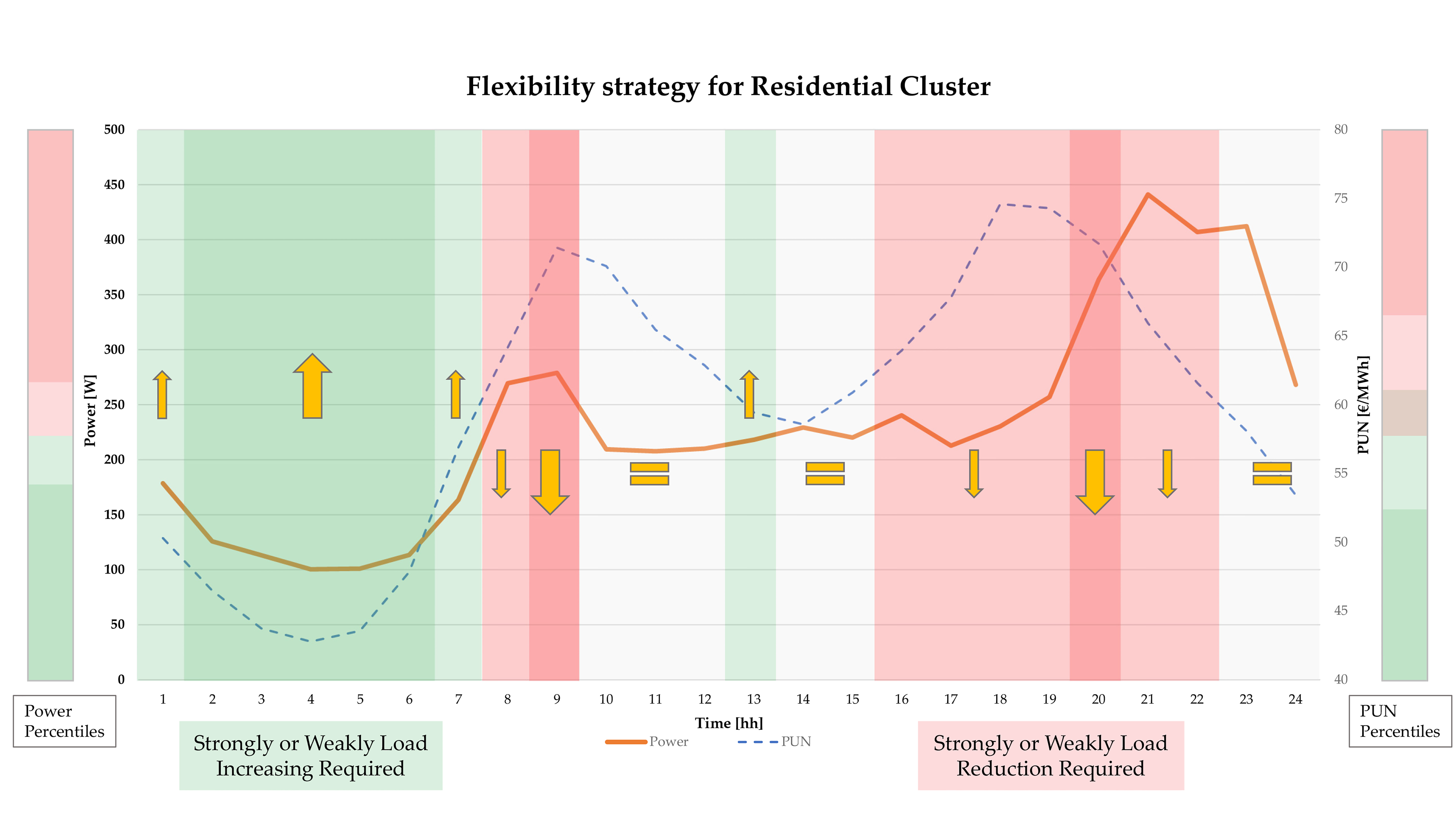
3.4. Loads Time-Shifting Strategy Identification

In this section, the implications associated to such a load time-shifting strategy implementation has been addressed and discussed. It is important to point out that the shifting command is delivered to end-users once both threshold conditions on price and power (i.e., on PUN Index value and on average uptake value) are verified. Those thresholds conditions can change dynamically, since their values are calculated in terms of percentiles, according to the Equation (2), and they are strongly dependent on the database content. Indeed, the generic index I_k associated to the desired percentile (e.g., fixing 35th percentile it entails I_k equal to I₃₅) has been calculated as follows:

$$I_k=\left[0.5+\left(n·\frac{k}{100}\right)\right]$$

(2)

where n indicates the number of ordinated sample data.

Having said, the boundary conditions to perform these simulations are summarised in a systemic overview in Appendix B.

Therefore, the Load Shifting Command Function ($LSCF=f\left(PUN, P\right)$) reads as:

$$\begin{array}{l}If (PUN>Limit 1) \wedge (P>Limit 1)then LSCF=-2\\ Else If (PUN>Limit 2) \wedge (P>Limit 2)then LSCF=-1\\ Else If (PUN<Limit 4) \wedge (P<Limit 4)thenLSCF=2\\ Else If (PUN<Limit 3) \wedge (P<Limit 3)thenLSCF=1\\ Else LSCF=0\\ EndIf\\ EndIf\\ EndIf\\ EndIf\end{array}$$

(3)

Numerical indicators ranging between −2 and 2 have been used to encode the load shifting commands when the limit thresholds are overcome, according to Equation (3). In detail, once PUN Index and Power are higher than the Limit 1, together with the other conditions, the command function provides −2 as output, suggesting the strong load reduction; when the Limit 2 is overcome, the output value is equal to −1, entailing a weak load reduction. On the contrary, weak load increase and strong load increase are suggested for all those values lower than the Limit 3 and laying in the band between Limit 3 and Limit 4, corresponding to 1 and 2, respectively. Finally, according to the flow chart reported in Figure 2 the last used value is 0, corresponding to no-load variation. As a consequence, the load shifting commands distribution have been plotted in Figure 16, Figure 17 and Figure 18. Applying that methodology it emerges that in the weekdays loads shifting from the evening hours (in the time span 8:00 p.m.–10:00 p.m.) towards the night hours (between 2:00 a.m. and 6:00 a.m.) as well as from the morning hours (8:00 a.m.–9:00 a.m.) towards the afternoon (1:00 p.m.–2:00 p.m.), are recommended (see Figure 16).

In the Saturdays case, the applied strategy recommends loads shifting from the evening hours (from 8:00 p.m. to 10:00 p.m.) towards the night hours (from 3:00 a.m. to 6:00 a.m.) and from the morning hours (10:00 a.m.–11:00 a.m.) towards the central hours of the day (12:00 a.m.–1:00 p.m.). Compared to the weekdays, a greater uncertainty in defining the strategy has been identified. Furthermore, a non-homogeneous commands’ distribution between cold and hot season, can be noticed according to Figure 17.

Finally, in the non-working days case, the electric loads occurring in the evening hours (from 7:00 p.m. to 11:00 p.m.) can be moved forward in the night-time (from 3:00 a.m. to 7:00 a.m.). Compared to the previous cases, the load shifting from the morning hours towards the afternoon it is not always required (see Figure 18).

3.5. Flexibility Indicators Calculation

In order to verify the load shifting strategy suitability, several monthly and yearly indicators have been calculated in this section.

Firstly, the average shiftable loads amount for the Residential Cluster (RC) emerging from the applied flexibility strategy has been evaluated.

Referring to each day typology, the suggested loads to move backward or forward have been calculated by the Equation (4), considering only the positive differences in the round brackets.

$$LS={\displaystyle \sum }_{i=1}^{24}(P_i-\overline{P})·\tau$$

(4)

Here, P_i represents the required power at the i-th hour, while the second term corresponds to the average power of RC profile, and τ is the time span (in this case equal to 1 h).

Secondly, the amount of potential available loads has been deduced from simulations results reported in Table 6. Thus, having supposed in a first approximation that these loads are evenly distributed over the day, the average amount related to each component constituting the RC, is equal to 1966 Wh/day. That value has been, substantially, deduced by dividing the whole flexibility potential of dwelling cluster (i.e., storable loads and shiftable loads) by its sample units (i.e., 751).

The comparison between the flexibility strategy suggestions and the available flexible loads is shown in Figure 19. It can be noticed that the calculated flexible loads are always lower than the available ones. As a consequence, the implemented strategy is suitable in any cases, showing the greater potential in the winter season over the non-working days.

Finally, once the Load Shifting (LS) function is calculated, it is possible to evaluate which is the Flexibility Index (FI_m) referred to the average day trend of each month. That parameter can be evaluated according to the Equation (5), where EN_m is the energy need over 24 h related the m-th month.

$$F{I}_m=\frac{L{S}_m}{E{N}_m}$$

(5)

Using the same definition, the Flexibility Index (FI_y) over the whole year is computable as a weighted average of Flexibility Index by month, in accordance with the Equation (6).

$$F{I}_y=\frac{{{\displaystyle \sum }}_{m=1}^{12}L{S}_m}{{{\displaystyle \sum }}_{m=1}^{12}E{N}_m}={\displaystyle \sum }_{m=1}^{12}F{I}_m·w_m$$

(6)

$$w_m=\frac{E{N}_m}{{{\displaystyle \sum }}_{m=1}^{12}E{N}_m}$$

(7)

Additionally, since the Available Shiftable Loads (ASL) is known, it is possible to define the Available Flexibility Index by month and by year as follows:

$$AF{I}_m=\frac{AS{L}_m}{E{N}_m}$$

(8)

$$AF{I}_y=\frac{AS{L}_{tot}}{{{\displaystyle \sum }}_{m=1}^{12}E{N}_m}$$

(9)

This latter parameter has been computed for the present RC and it is equal to 37.7%. Then, in order to evaluate the effectiveness of the adopted strategy, the Flexibility Index and the Available Flexibility Index can be correlated by Equations (10) and (11).

$${\epsilon }_m=\frac{F{I}_m}{AF{I}_m}$$

(10)

$${\epsilon }_y=\frac{F{I}_y}{AF{I}_y}$$

(11)

Figure 20 depicts the strategy effectiveness values ${\epsilon }_m$, sorting the results by month and day typologies as usual. Thereafter, all those performance values can be outlined by calculating the effectiveness over the year ${\epsilon }_y$, which is equal to 0.34 for this case.

However, once the actual hourly distribution of the available shiftable loads is known, it is possible to assess also the intraday strategy effectiveness. It is important to point out that the results of these comparisons are evidently dependent on the specific choice of threshold limits in the strategy definition. In this case, their values have been deduced from the statistical analysis carried out on both the cluster load and PUN Index, assuming also an identical definition for the variables.

Since it has been assumed Limit 2 = Limit 3 = 50th percentile, it implies that, in all those cases where those thresholds are overcome, a load reduction is recommended; on the contrary, beneath the limits the load increase is required. More generally, this is a conservative strategy, given that any other choice would lead to higher differences between the available and the effective shiftable loads, penalising the strategy effectiveness.

However, it is necessary to verify the precise hourly distribution of the available flexible loads, instead of considering them equally distributed over the 24 h. Furthermore, it is important to take into account where the household appliances operational constraints occur to limit the lowering of flexible loads amount. Indeed, the adoption of a flexibility strategy should not negatively affect the end user’s wellbeing, and it must consider the correlations between appliance operation and the occupant presence (i.e., vacuum cleaner, iron, etc.). Those issues have not been extensively addressed in this work, but they will be deeply discussed in the further development of the research project. Anyway, it is noteworthy that accounting for additional operating constraints on household appliances will reduce the flexibility indexes as well as the strategy effectiveness.

4. Conclusions

The DR activities application to the residential sector represents a viable option to get a higher cost effectiveness for both utilities and end-users. By creating a dwelling cluster, it is possible to gather huge amounts of flexible loads to be shifted over the daytime, in order to participate actively to the market outcomes.

In this work, a procedure to build a dwelling cluster load profile has been presented and discussed, on the basis of a combined approach: the experimental measurements have been coupled with the statistical analysis. Referring to the Italian context, that approach could represent a good opportunity, on one hand to update available data, on the other hand to develop new models for the low voltage grid management.

Finally, a flexibility strategy has been implemented along with the definition of several performance indicators. Using the Italian residential sector as a reference case, and the Italian electricity price trend over 2018 and 2019, it has been possible to evaluate the dwellings contribution to a more flexible system. The most remarkable findings can be listed as follows:

• 14 dwelling archetypes have been defined by the use of a numerical approach based on a grade scale ranging between 0 and 1; each sample household (i.e., 751) has been compared to the archetypes in order to identify its category; this method leads to a good fitting since, on average, the best grade is equal to 0.81;
• the most representative archetypes, in terms of the highest number of dwellings belonging to them, are the #9, #6, and #5 corresponding to 165, 138, and 102 sample households, respectively;
• from data collected by a survey, the available potential of flexibility related to the dwellings cluster has been calculated and it is equal to 538.95 MWh/year; therefore, the average daily value of flexible loads per dwelling is equal to 1966 Wh/d;
• by simulating a flexible strategy on an RC of Italian residential sector, which is based on the hourly pricing mechanism following the day-ahead market outcomes, and on limitations of power uptakes, monthly and annual indicators have been defined; so doing, the flexible strategy effectiveness can be computed to assess its actual suitability;
• the highest monthly effectiveness values have been registered in the cold season over the non-working days ranging between 0.49 and 0.53. Conversely, in the hot season, the maximum effectiveness values are generally lower compared to the winter ones (i.e., 0.3–0.4) and they occur over the weekdays. In the end, all those results can be outlined by means of a single indicator (annual effectiveness), which, in this case, is 0.34.

The calculated values relative to the management effectiveness indicate (at the outset) that the proposed management strategy for the Italian residential sector can be applied. Further developments of present work will be focused on identifying the realistic time distribution of the available flexible loads, and matching the user wellbeing and the appliances technical constraints, due to their contemporary use. In so doing, it will be possible to evaluate more precisely the flexible loads magnitude (which is expected to be lower than the one in the present case study) and to recalculate strategy effectiveness for evaluating actual suitability.

Moreover, the algorithm to identify the electricity peak price variation deriving from the DR strategies adoption has to be implemented. Similarly, a workflow definition associated to the Information and Communication Technologies (ICT) infrastructure has to be built in order to identify and select how many users can effectively apply the load time shifting commands. Finally, evolutive scenarios involving the heating system and DHW electrification, by means of heat pump wide deployment in the Italian residential sector, will be performed and analysed.

References

1. European Commission. A Clean Planet for all A European Strategic Long-Term Vision for a Prosperous, Modern, Competitive and Climate Neutral Economy. 2018. Available online: https://ec.europa.eu/clima/sites/clima/files/docs/pages/com_2018_733_en.pdf (accessed on 13 April 2019).
2. Brouwer, A.S.; Van Den Broek, M.; Seebregts, A.; Faaij, A. Impacts of large-scale Intermittent Renewable Energy Sources on electricity systems, and how these can be modeled. Renew. Sustain. Energy Rev. 2014, 33, 443–466. [Google Scholar] [CrossRef]
3. Palensky, P.; Dietrich, D. Demand side management: Demand response, intelligent energy systems, and smart loads. IEEE Trans. Ind. Informatics 2011, 7, 381–388. [Google Scholar] [CrossRef] [Green Version]
4. Strbac, G. Demand side management: Benefits and challenges. Energy Policy 2008, 36, 4419–4426. [Google Scholar] [CrossRef]
5. Behrangrad, M. A review of demand side management business models in the electricity market. Renew. Sustain. Energy Rev. 2015, 47, 270–283. [Google Scholar] [CrossRef]
6. Schibuola, L.; Scarpa, M.; Tambani, C. Demand response management by means of heat pumps controlled via real time pricing. Energy Build. 2015, 90, 15–28. [Google Scholar] [CrossRef]
7. Diesendorf, M.; Elliston, B. The feasibility of 100% renewable electricity systems: A response to critics. Renew. Sustain. Energy Rev. 2018, 93, 318–330. [Google Scholar] [CrossRef]
8. Zappa, W.; Junginger, M.; van den Broek, M. Is a 100% renewable European power system feasible by 2050? Appl. Energy. 2019, 233, 1027–1050. [Google Scholar] [CrossRef]
9. Eurostat. Statistics | Eurostat, (n.d.). Available online: https://ec.europa.eu/eurostat/databrowser/view/ten00124/default/table?lang=en (accessed on 31 March 2020).
10. Energy Efficiency Trends & Policies | ODYSSEE-MURE, (n.d.). Available online: https://www.odyssee-mure.eu/ (accessed on 20 May 2020).
11. Jensen, S.Ø.; Marszal-Pomianowska, A.; Lollini, R.; Pasut, W.; Knotzer, A.; Engelmann, P.; Stafford, A.; Reynders, G. IEA EBC Annex 67 Energy Flexible Buildings. Energy Build. 2017, 155, 25–34. [Google Scholar] [CrossRef] [Green Version]
12. Rahmani-Andebili, M. Scheduling deferrable appliances and energy resources of a smart home applying multi-time scale stochastic model predictive control. Sustain. Cities Soc. 2017, 32, 338–347. [Google Scholar] [CrossRef]
13. Chen, Y.; Xu, P.; Gu, J.; Schmidt, F.; Li, W. Measures to improve energy demand flexibility in buildings for demand response (DR): A review. Energy Build. 2018, 177, 125–139. [Google Scholar] [CrossRef]
14. Cumo, F.; Curreli, F.R.; Pennacchia, E.; Piras, G.; Roversi, R. Enhancing the urban quality of life: A case study of a coastal city in the metropolitan area of Rome. WIT Trans. Built Environ. 2017, 170, 127–137. [Google Scholar] [CrossRef] [Green Version]
15. Péan, T.; Costa-Castelló, R.; Salom, J. Price and carbon-based energy flexibility of residential heating and cooling loads using model predictive control. Sustain. Cities Soc. 2019, 50, 101579. [Google Scholar] [CrossRef]
16. Vázquez, F.V.; Koponen, J.; Ruuskanen, V.; Bajamundi, C.; Kosonen, A.; Simell, P.; Ahola, J.; Frilund, C.; Elfving, J.; Reinikainen, M.; et al. Power-to-X technology using renewable electricity and carbon dioxide from ambient air: SOLETAIR proof-of-concept and improved process concept. J. CO2 Util. 2018, 28, 235–246. [Google Scholar] [CrossRef]
17. Irena. Innovation Landscape for a Renewable-Powered Future: Solutions to Integrate Variable Renewables. 2019. Available online: www.irena.org/publications (accessed on 25 June 2020).
18. The European Parliament and the Council of the European Union, Directive 2014/94/eu of the European Parliament and of the Council—of 22 October 2014—on the Deployment of Alternative Fuels Infrastructure. Available online: https://eur-lex.europa.eu/legal-content/EN/TXT/PDF/?uri=CELEX:32014L0094&from=en (accessed on 30 June 2020).
19. De Santoli, L.; Basso, G.L.; Garcia, D.A.; Piras, G.; Spiridigliozzi, G. Dynamic simulation model of trans-critical carbon dioxide heat pump application for boosting low temperature distribution networks in dwellings. Energies 2019, 12, 484. [Google Scholar] [CrossRef] [Green Version]
20. Mazzoni, S.; Ooi, S.; Nastasi, B.; Romagnoli, A. Energy storage technologies as techno-economic parameters for master-planning and optimal dispatch in smart multi energy systems. Appl. Energy. 2019, 254, 113682. [Google Scholar] [CrossRef]
21. Nastasi, B. Hydrogen policy, market, and R&D projects. In Solar Hydrogen Production: Processes, Systems and Technologies; Calise, F., D’Accadia, M.D., Santarelli, M., Lanzini, A., Ferrero, D., Eds.; Academic Press: Cambridge, MA, USA, 2019; pp. 31–44. [Google Scholar] [CrossRef]
22. Nastasi, B.; Lo Basso, G.; Astiaso Garcia, D.; Cumo, F.; de Santoli, L. Power-to-gas leverage effect on power-to-heat application for urban renewable thermal energy systems. Int. J. Hydrog. Energy. 2018, 43, 23076–23090. [Google Scholar] [CrossRef]
23. Roversi, R.; Cumo, F.; D’Angelo, A.; Pennacchia, E.; Piras, G. Feasibility of municipal waste reuse for building envelopes for near zero-energy buildings. WIT Trans. Ecol. Environ. 2017, 224, 115–125. [Google Scholar] [CrossRef] [Green Version]
24. Lezama, F.; Faia, R.; Faria, P.; Vale, Z. Demand Response of Residential Houses Equipped with PV-Battery Systems: An Application Study Using Evolutionary Algorithms. Energies 2020, 13, 2466. [Google Scholar] [CrossRef]
25. D’Ettorre, F.; De Rosa, M.; Conti, P.; Testi, D.; Finn, D. Mapping the energy flexibility potential of single buildings equipped with optimally-controlled heat pump, gas boilers and thermal storage. Sustain. Cities Soc. 2019, 50, 101689. [Google Scholar] [CrossRef]
26. Goy, S.; Finn, D. Estimating demand response potential in building clusters. Energy Procedia 2015, 78, 3391–3396. [Google Scholar] [CrossRef] [Green Version]
27. Adhikari, R.; Pipattanasomporn, M.; Rahman, S. An algorithm for optimal management of aggregated HVAC power demand using smart thermostats. Appl. Energy. 2018, 217, 166–177. [Google Scholar] [CrossRef]
28. Cai, H.; Ziras, C.; You, S.; Li, R.; Honoré, K.; Bindner, H.W. Demand side management in urban district heating networks. Appl. Energy. 2018, 230, 506–518. [Google Scholar] [CrossRef]
29. D’hulst, R.; Labeeuw, W.; Beusen, B.; Claessens, S.; Deconinck, G.; Vanthournout, K. Demand response flexibility and flexibility potential of residential smart appliances: Experiences from large pilot test in Belgium. Appl. Energy. 2015, 155, 79–90. [Google Scholar] [CrossRef]
30. Caputo, P.; Gaia, C.; Zanotto, V. A Methodology for Defining Electricity Demand in Energy Simulations Referred to the Italian Context. Energies 2013, 6, 6274–6292. [Google Scholar] [CrossRef]
31. Ferrari, S.; Zagarella, F. Assessing Buildings Hourly Energy Needs for Urban Energy Planning in Southern European Context. Procedia Eng. 2016, 161, 783–791. [Google Scholar] [CrossRef] [Green Version]
32. Ferrari, S.; Zanotto, V. Defining representative building energy models. In Building Energy Performance Assessment in Southern Europe; Ferrari, S., Zanotto, V., Eds.; Springer: Cham, Switzerland, 2016. [Google Scholar] [CrossRef]
33. Commission of the European Communities. Demand-Side Management: End-Use Metering Campaign in 400 Households of the European Community, Assessment of the Potential Electricity Savings. Project EURECO, SAVE Programme. Available online: http://www.eerg.it/resource/pages/it/Progetti_-_MICENE/finalreporteureco2002.pdf (accessed on 30 June 2020).
34. Fumagalli, S.; Pizzuti, S.; Romano, S. Smart Homes Network: Sviluppo dei servizi di aggregazione e progettazione di un dimostrativo pilota. ENEA Ric. Di Sist. Elettr. 2016. Available online: https://www.enea.it/it/Ricerca_sviluppo/documenti/ricerca-di-sistema-elettrico/adp-mise-enea-2015-2017/smart-district-urbano/rds_par2016_006.pdf (accessed on 23 April 2020).
35. Shariatzadeh, F.; Mandal, P.; Srivastava, A.K. Demand response for sustainable energy systems: A review, application and implementation strategy, Renew. Sustain. Energy Rev. 2015, 45, 343–350. [Google Scholar] [CrossRef]
36. Hussain, I.; Mohsin, S.; Basit, A.; Khan, Z.A.; Qasim, U.; Javaid, N. A review on demand response: Pricing, optimization, and appliance scheduling. Procedia Comput. Sci. 2015, 52, 843–850. [Google Scholar] [CrossRef] [Green Version]
37. Haider, H.T.; See, O.H.; Elmenreich, W. A review of residential demand response of smart grid. Renew. Sustain. Energy Rev. 2016, 59, 166–178. [Google Scholar] [CrossRef]
38. Mancini, F.; Lo Basso, G.; De Santoli, L. Energy use in residential buildings: Characterisation for identifying flexible loads by means of a questionnaire survey. Energies 2019, 12, 2055. [Google Scholar] [CrossRef] [Green Version]
39. Mancini, F.; Nastasi, B. Energy retrofitting effects on the energy flexibility of dwellings. Energies 2019, 12, 2788. [Google Scholar] [CrossRef] [Green Version]
40. Mancini, F.; Lo Basso, G.; de Santoli, L. Energy use in residential buildings: Impact of building automation control systems on energy performance and flexibility. Energies 2019, 12, 2896. [Google Scholar] [CrossRef] [Green Version]
41. Mancini, F.; Lo Basso, G. How climate change affects the building energy consumptions due to cooling, heating, and electricity demands of Italian residential sector. Energies 2020, 13, 410. [Google Scholar] [CrossRef] [Green Version]
42. UNI Ente Italiano di Normazione. Italian Technical Standard UNI/TS 11300-1:2014—Energy Performance of Buildings—Evaluation of Energy Need for Space Heating and Cooling, (n.d.). Available online: http://store.uni.com/catalogo/index.php/uni-ts-11300-1-2014.html (accessed on 18 September 2019).
43. Suomalainen, K.; Eyers, D.; Ford, R.; Stephenson, J.; Anderson, B.; Jack, M. Detailed comparison of energy-related time-use diaries and monitored residential electricity demand. Energy Build. 2019, 183, 418–427. [Google Scholar] [CrossRef] [Green Version]
44. Eurostat. Energy Consumption in Households—Statistics Explained. Available online: https://ec.europa.eu/eurostat/statistics-explained/index.php?title=Energy_consumption_in_households (accessed on 20 May 2020).
45. Marszal-Pomianowska, A.; Heiselberg, P.; Larsen, O.K. Household electricity demand profiles—A high-resolution load model to facilitate modelling of energy flexible buildings. Energy 2016, 103, 487–501. [Google Scholar] [CrossRef]
46. Oliveira Panão, M.J.N.; Brito, M.C. Modelling aggregate hourly electricity consumption based on bottom-up building stock. Energy Build. 2018, 170, 170–182. [Google Scholar] [CrossRef]
47. Pasichnyi, O.; Wallin, J.; Kordas, O. Data-driven building archetypes for urban building energy modelling. Energy 2019, 181, 360–377. [Google Scholar] [CrossRef]
48. Buttitta, G.; Turner, W.; Finn, D. Clustering of Household Occupancy Profiles for Archetype Building Models. Energy Procedia 2017, 111, 161–170. [Google Scholar] [CrossRef]
49. Wang, A.; Li, R.; You, S. Development of a data driven approach to explore the energy flexibility potential of building clusters. Appl. Energy. 2018, 232, 89–100. [Google Scholar] [CrossRef]
50. GME, Excel Historical Data. 2018. Available online: https://www.mercatoelettrico.org/en/download/DatiStorici.aspx (accessed on 30 March 2020).
51. Pallonetto, F.; Oxizidis, S.; Milano, F.; Finn, D. The effect of time-of-use tariffs on the demand response flexibility of an all-electric smart-grid-ready dwelling. Energy Build. 2016, 128, 56–67. [Google Scholar] [CrossRef]
52. Cortés-Arcos, T.; Bernal-Agustín, J.L.; Dufo-López, R.; Lujano-Rojas, J.M.; Contreras, J. Multi-objective demand response to real-time prices (RTP) using a task scheduling methodology. Energy 2017, 138, 19–31. [Google Scholar] [CrossRef]
53. Kühnlenz, F.; Nardelli, P.H.J.; Karhinen, S.; Svento, R. Implementing flexible demand: Real-time price vs. market integration. Energy 2018, 149, 550–565. [Google Scholar] [CrossRef] [Green Version]
54. GME—Glossary, (n.d.). Available online: http://www.mercatoelettrico.org/en/tools/glossario.aspx#Prices (accessed on 17 June 2020).
55. European Central Bank. ECB Euro Reference Exchange Rate: US Dollar (USD), ECB/ Eurosystem Policy Exch. Rates. 2019. Available online: https://www.ecb.europa.eu/stats/policy_and_exchange_rates/euro_reference_exchange_rates/html/eurofxref-graph-usd.en.html (accessed on 20 May 2020).
Figure 1. Flow chart related to the methodological approach.
Energies 13 03359 g001
Figure 2. Flow chart related to the consumptions’ optimization process (PUN: National Unique Price).
Energies 13 03359 g002
Figure 3. Building subdivision. (a) Household size. (b) Family occupancy.
Energies 13 03359 g003
Figure 4. Heating system typologies: (a) inner Space heating; (b) DHW.
Energies 13 03359 g004
Figure 5. Control kit layout.
Energies 13 03359 g005
Figure 6. Archetypes average daily profiles over the weekdays.
Energies 13 03359 g006
Figure 7. Archetypes average daily profiles over the Saturdays.
Energies 13 03359 g007
Figure 8. Archetypes average daily profiles over non-working days.
Energies 13 03359 g008
Figure 9. Best fitting statistic distribution.
Energies 13 03359 g009
Figure 10. The aggregate profile of average power: weekdays. (Green: low; White: medium; Red: high).
Energies 13 03359 g010
Figure 11. The aggregate profile of average power: Saturdays. (Green: low; White: medium; Red: high).
Energies 13 03359 g011
Figure 12. The aggregate profile of average power: non-working days. (Green: low; White: medium; Red: high).
Energies 13 03359 g012
Figure 13. Average PUN Index trend over the reference months: weekdays. (Green: low; White: medium; Red: high).
Energies 13 03359 g013
Figure 14. Average PUN Index trend over the reference months: Saturdays. (Green: low; White: medium; Red: high).
Energies 13 03359 g014
Figure 15. Average PUN Index trend over the reference months: non-working days. (Green: low; White: medium; Red: high).
Energies 13 03359 g015
Figure 16. Strategy to optimise the load shifting: weekdays; (−2, Green) Strong Load reduction; (−1, Light Green) Weak Load reduction; (0, White) No Load variation; (1, Light Red) Weak Load increase; (2, Red) Strong Load increase.
Energies 13 03359 g016
Figure 17. Strategy to optimise the load shifting: Saturdays. (−2, Green) Strong Load reduction; (−1, Light Green) Weak Load reduction; (0, White) No Load variation; (1, Light Red) Weak Load increase; (2, Red) Strong Load increase.
Energies 13 03359 g017
Figure 18. Strategy to optimise the load shifting: non-working days. (−2, Green) Strong Load reduction; (−1, Light Green) Weak Load reduction; (0, White) No Load variation; (1, Light Red) Weak Load increase; (2, Red) Strong Load increase.
Energies 13 03359 g018
Figure 19. Daily load shifting deriving from the strategy application by month and day typologies. The dot line represents the available daily shiftable loads to participate at the flexibility mechanism.
Energies 13 03359 g019
Figure 20. Strategy effectiveness sorted by month and day typologies.
Energies 13 03359 g020