Abstract
When planning the energy demand of ventilation, proper consideration should be given to the possible scenarios of indoor air quality and pollutant concentrations. The purpose of the present research is to create a practical method of prioritising indoor air pollutants, considering technical, economical and health aspects, in the Indoor Air Quality model (IAQ). In order to find the global weights for the combined IAQindex model sub-elements (in practice, air pollutant concentrations), the Multi-Criteria Decision Making (MCDM) approach is used. The authors have approached the problem of a weighting scheme in a model such as the complex model of the IAQ related to making decisions with many criteria and with the Multi-Attribute Decision Making MADM approach (specifically MCDM). The basis of the MADM method is a decision matrix constructed rationally by the authors, which includes six attributes: actual indoor air carbon dioxide concentration, total volatile organic compounds (TVOCs) and formaldehyde HCHO concentration, and their anthropogenic and construction product emissions to the indoor environment. The decision model of IAQindex includes five alternatives (possible situations), and the combination of pollutant concentration attributes with additional emission attributes is related to the indoor environment under specific situation. For defining the weights of criteria, the authors provide objective approaches: (i) entropy-based approach considering measuring the amount of information, and (ii) CRITIC, a statistic-based approach. The value of the presented method, i.e., the determination of global weights for IAQ components, is shown as a practical application to determine IAQ and the Indoor Environmental Quality (IEQ) index for an office building used as a case study.
1. Introduction and Literature Review
1.1. Research Problem
In literature on the Multi-Attribute Decision Making (MADM )method, the combined Indoor Air Quality (∑IAQ) model optimisation problem has not been addressed thus far to set up the weights of model sub-components (in practice due to excess indoor pollutant concentrations and risk to occupants). One of the main criteria for optimising such a decision problem should be, directly or indirectly, the cost of ventilation for the elimination of excess pollution concentrations. For the purposes of the decision problem, it is assumed that the general criterion for optimising such a weighing system is to include a range of IAQ indicators and components, i.e., types of contaminants that are most important due to health and toxicity or the amount of air to be removed by the ventilation system.
The MADM method, as a specific kind of Multi-Criteria Decision Making (MCDM) approach, has emerged as a formal methodology for assessing available information and providing values supporting decision-makers in many areas, including environmental engineering. The published results suggest that, over the past decade, there has been a significant increase in the use of MCDM in technical areas for civil engineering applications, the design of indoor environments and the improvement of outdoor environments [1]. MCDM makes it possible to assess complicated decision problems limited by numerous and divergent criteria based on expert subjective assessments (subjective weights) and decision models, the purposes of which are to calculate objective weights according to the rules of decision theory and order multiple parameters of the analysed problem. Recently, the construction industry has become one of the main stressors to the environment and society globally [2]. In the context of the continuous decrease in energy consumption by new buildings and the fundamental need to provide comfortable and healthy conditions for the users in indoor environments, there is a growing urgency to use IAQ models that meet certain criteria. IAQ models are the main components of building Indoor Environmental Quality models [3] and increasingly used for building design software (such as Building Information Modelling, BIM) or as part of building managing systems (BMSs) controlling heat, cooling and ventilation systems (HVACs).
The basic aim of this study was to develop a new approach which combines the previously developed ΣIAQ model [4], containing loosely connected components (indoor air pollution elements and their impact on user perception), with a new weighting system based on MADM that would produce a practical tool supporting choices of the best possible indoor environment and air control strategy. As a case study, a large office building was used, for which the authors had already assessed the indoor environmental parameters [4,5], and the authors recalculated the ΣIAQ and Indoor Environmental Quality (IEQ) indices using the new weighting scheme. A similar issue for the external environment was presented in [6]. This team built the MCDM decision model to study the impacts of outdoor air pollution on the economic development of selected zones in China.
How humans perceive indoor comfort is a complex phenomenon. Authors have analysed the problem from a holistic point of view following current developments described widely [3,4,5]. Researchers assessing indoor comfort in buildings have focused primarily on optimizing individual components of the indoor environment (thermal, light and acoustic comfort, and air quality), as these four parameters connected to the human senses are considered by occupants to be the most important in determining their comfort [3]. Our research work is aimed at identifying the relationship between the indoor parameters and the resulting reactions of building occupants (in particular, in the area of IAQ). This multi-component approach to indoor comfort focuses on the ‘human stimuli response’ and has led to well-known indoor comfort models such as the thermal comfort model developed by Fanger. In recent years, this holistic approach to the indoor environment has been presented in the European standard EN 15251 and later in EN 16798-1: 2018 [7] where, for the first time, a wider number of indoor comfort criteria were considered. These standards suggest an approach to the classification of IAQ and IEQ models and support certification of buildings taking into account specific components of indoor environment, however, they do not provide a practical guidance or an approach on how to combine them into one indicator that could be useful to classify indoor environmental conditions. The authors solved this problem in a previous publication [4]. When the predominant indoor pollutants have different characteristic values, there is a large problem regarding the choice and weighting method of IAQ sub-components. The problem is considered in this article with use of the MADM approach. Taking into consideration the characteristics and correlations of the selected pollutants, IAQ may be characterized by representative indicators. Our studies on Building Research Establishment Environmental Assessment Method (BREEAM)certified buildings [5] and Leadership in Energy and Environmental Design (LEED) system shown out that carbon dioxide, total volatile organic compounds (TVOCs) and HCHO are the main worldwide, independent and representative environmental indicators. They are being used worldwide as an evaluation index of IAQ in buildings (mainly offices with mechanical ventilation). Since each of these indicators represents a pollutant class with comparable indoor sources and characteristic dissemination and the indexed group avoids unreliable measurements. This is based on the fact that indicators are “too small” because of decreased critical concentrations. A method of data pre-treatment is proposed by us in the procedures, which reflects concentration differences between pollutants and considerstheir influence on the satisfaction of the building users. Taking into consideration the existing knowledge gap, the authors proposed an objective method to determine weights in theIAQ model in this article. The article provides the procedure to calculate global weights for the IAQ model sub-components. The ΣIAQ model considers the impact of air concentrations of selected air pollutants (CO2, TVOCs, HCHO, etc.) on the building users’ perceptions. The weighted IAQ model was developed by the authors considering the standard EN 16798-1:2019 [7] provisions with the intention to create it as a main sub-component of the overall Indoor Environmental Quality (IEQ) model [8,9] with assumptions described in references [3,8]. The IAQ model and weight system applies to office buildings with mechanical ventilation. Quasi-static indoor environment conditions and full air mixing in the building are assumed.
1.2. Basic Information on the MADM Approach
Some analogies to the presented IAQ weighting problem can be found in the literature, and the studies described so far have led to the establishment of rankings of alternative solutions to the decision problem. The MADM method has beenused as an effective tool for choosing the optimal composition of construction materials [10,11], estimating their weights [12] for the selection of the optimal air filtration method to remove pollutants [13], and choosing the optimal set of indoor environment parameters in an office building [14] when the alternatives are differently dated combinations of these parameters (attributes). Additionally, the MADM technique solved the problem of the impact of air pollution on the level of economic development of Chinese cities (for example, the city of Wuhan) [6]. This project is interesting to the authors because it concerns the impact of air pollution. The research involved determining the weights of air pollutants of various types of VOCs, and of the physical parameters affecting these pollutants (attributes of the decision problem), and establishing a ranking of the specific systems of these environmental parameters occurring in different years (alternatives to the decision problem). In these simulations, a modified Technique for Order of Preference by Similarity to Ideal Solution (TOPSIS) was used. This approach uses neural networks to determine weights.
MCDM was also proposed inchoosing a strategy to design sustainable buildings [15]. The purpose of this study was to provide a method combiningclimate changeeffects, adaptive thermal satisfaction, life cycle assessment (LCA), life cycle cost (LCC) analysis and multi-criteria decision making in order to set the most valuable design strategy that would improve building object sustainability. For the assessment and selection of the most appropriate design strategies for buildings, attributes were analysed using a multi-disciplinary approach based on sustainability criteria. In order to find the best building design strategy and make decisions based on several criteria, the Complex Proportional Assessment (COPRAS) method was used [16,17]. This method [15] assumes proportional and direct dependence of the significance of the usability degree of the tested versions of buildings (alternatives) in the system of criteria (attributes) described by the parameters: (1) hours of comfort in the room, (2) primary energy demand, (3) CO2 emissions, and (4) costs). This method was successfully used to deal with the complex selection of problems. Based on this study, by using the COPRAS method, the authors provided a ranking of the most valuable structural solutions for buildings that meet four characteristic parameters/criteria and their weights built within the decision model.
Most often, MCDM decision models have been used by researchers in the process of selecting components of construction materials by methods such as the “preference technique in classification according to the similarity to the ideal solution” (TOPSIS) [18,19], which uses the principles of analytical hierarchy process (AHP) [17] and various versions of Elimination and Choice Expressing the Reality (ELECTRE) [1]. The method using entropic weights, created on the basis of Shannon’s information theory [20] for the selection of materials [10,11], was also used. Additionally, the method of material selection from many alternatives based on Jahan’s research [12] and the analysis of correlation between Criteria Importance Through Intercriteria Correlation (CRITIC) criteria [12] was used. Alemi-Ardakani [10] analysed the possibilities of optimising the composition of composite materials using the Adjustable Mean Bars (AMB), Modified Digital Logic (MDL), Numeric Logic (NL) and CRITIC [10] methods, as well as the Peng method [21] of creating rankings of preference functions using composition enrichment technology (PROMETHEE—Preference Ranking Organization Method for Enrichment Evaluations) or a preference selection indicator [1].
MCDM methods have now become so popular for extending knowledge of environmental impacts and sustainable construction that several groups of scientists reviewed the applications and development trends of decision models in “environmental sciences” (Cegan, Linkov et al., 2011 [22] and 2017 [23]) and in sustainable construction (Navarro et al. 2019 [1]).MADM methods are a special case of MCDM methods in which decision-making criteria have been replaced by attributes, i.e., features of problems or processes that are evaluated by analysts. Each MADM technique has its own specifics, assumptions and principles. Almost all of the above-mentioned MCDM methods are characterised by the complexity of the mathematics of their moderate to extreme models. Application of these techniques is difficult, requiring advanced mathematical skills and knowledge. Therefore, the creation of undemanding MADM methods is highly desirable. Multi-purpose optimisation based on proportion analysis, named Multi-Objective Optimization by Ratio Analysis(MOORA)was proposed by Brauers and Zavadskas (2006) [24] and is used for the selection of construction materials [25], as it involves uncomplicated mathematics. Therefore, it can be used effortlessly and effectively to choose the best materials or solutions.
To solve the weight problem in the IAQ model, the authors used two methods: entropy and CRITIC. The objective weighting measure was proposed with the Shannon entropy concept provided in [20]. In MCDM, the entropy relates to the diversity degree within the attribute data set. The higher this diversity degree, the higher the attribute weight. The smaller the entropy within the associated data to the attribute, the higher the power of discrimination of the attribute in changing ranks of alternatives. The entropy weights are calculated with only one set of values dedicated to the same attribute j in all alternative levels of the decision matrix. Entropy weight is a typical attribute weight, but it is always introduced to the global weight as a factor in all decision matrix indices. In the entropy method, an attribute with a performance rating that is very different from the others has more importance in the problem because it has a greater impact on ranking outcomes. The attribute has lesser importance if all attributes have comparable performance ratings for that attribute. An objective method to weigh criteria importance through inter-criteria correlation (CRITIC) based on the SD approach was proposed by Diakoulaki and later explored by Jahan [12]. The higher the level of interdependency between attributes, the larger the ranking outcome error. The CRITIC approach is a popular objective method to calculate weights, which solves the problem of interdependencies between the attributes in all combinations by considering the correlation between the sets of variables from various alternative levels, while calculating the weights. It is one of the objective methods of weight determination that belongs to the class of correlation methods. It uses the information contained in the data matrix in the form of the degree of deviation of a variant value from a given mean value of the criteria. The CRITIC method is particularly useful in the IAQ model, as we show later, because the parameters adopted as attributes in the decision model of this problem are the concentrations of selected pollutants and the emissions of the same pollutants; therefore, in the IAQ decision matrix there are correlating attributes.
1.3. Basic Information on the ∑IAQ Model
The ΣIAQ model, in which the authors are looking for objective weight sub-elements, uses a selected number of indoor air pollutants (P1, … j) and their impact on user dissatisfaction (Percentage Dissatisfied as PD = f(cj) in %). The combined ∑IAQindex (cumulative percentage of satisfied users with indoor air quality, including selected pollutant impacts of user perception) Equation is
where sub-indices ∑IAQ(Pj) are the percentage of users satisfied with the pollutant concentration; WP1, … Pj are weights for each IAQ sub-component for groups of air pollutants with comparable concentrations.
∑IAQindex = WP1·IAQ(P1)index + WP2∙IAQ(P2)index, …, WPj∙IAQ(Pj)index
There is a difference in Δcj concentration between the measured air concentration of pollutant cj and the recommended “reference” concentration cref (reference by the European Commission “safe” values such as cLCI or cELV), which may be below the actual air concentration in the contaminated rooms. Thus, the concentration excess related to the ventilation rate is
Δcj = cj − cref
The excess concentration weights WPj for the IAQ model until now have been calculated based on the arithmetic mean or by adjusting (normalization) all attribute Δcj values using Equation (3):
where the sum of the adjusted weights WP,j of all pollutants to be removed by ventilation should be in unity. This weighting scheme has been used by the authors in previous years, but in this article, we propose a better and more objective approach based on the MADM approach.
Three levels of complexity of the IAQ model were proposed, and in each, pollutants have been defined that were included in the IAQ model. Figure 1 shows the extended IAQquality model with its sub-indices and also with the sub-components of the IAQcomfort/health model type, i.e., indoor air pollutants important to health with an impact on the energy balance of a building using a mechanical ventilation system.
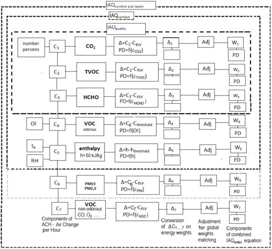
Figure 1.
Combined Indoor Air Quality (∑IAQ) model with weighting scheme; horizontally, the model is bound by the weighing processes of individual sub-models; vertically, the model is bound by a chain of input components (pollutant concentrations in ventilated indoor air) and a chain of output components (elements of the combined IAQindex equation).
The experimental dependencies of the percentage of persons dissatisfied (%PD, where %PD = 1-IAQ) and the concentrations values of air pollutants, cj, perceived in the adequate ranges are of fundamental significance to the sub-components relevant to the IAQ and IEQ models [9]. In the ΣIAQ model proposed by the authors, the accepted common approach is engaged to transform individual pollutant concentrations into sub-components before these are combined into a single index. The aggregated summary of sub-components, however, may lead to a situation in which all components are below the individual health threshold, but the final index shows that the health threshold is exceeded. Conversely, the averaging of partial sub-components may lead to an outcome whereby the overall index shows an acceptable IAQ value, but one or more partial indicators are higher than their individual health threshold. The solution proposed is to use all sub-component maximum values to provide a final form of the ∑IAQ. Considering this, we proposed the ∑IAQ model with three possible levels of model complication due to the application potential, as we show in Figure 2:
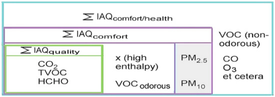
Figure 2.
The IAQ model with three complexity levels reflecting the application potential.
- building sustainable assessment schemes (like BREEAM assessment)—three sub-components, named quality, ΣIAQquality;
- design purpose, considering the perceptible pollutants affecting indoor satisfaction and comfort, with the intention to use this index for calculating the IEQ—five sub-components, called comfort, ΣIAQcomfort; and
- complex design purpose, where ∑IAQindex represents health and comfort (seven sub-components, or more if necessary), called comfort and health, ΣIAQcomfort/health.
The simplest IAQ index level can be used with the main purpose of supporting a sustainable building assessment and certification by using only three sub-components: CO2, HCHO and TVOC. ΣIAQquality model is used in this article to assess the office building (case study).
From the dependencies, expressed as the curves for the percentage of satisfied users with pollutant IAQ(CO2) or IAQ(VOCodorous), the following Equations (4)–(6) of the models are provided:
∑IAQquality = W1·IAQ(CO2) + W2·IAQ(TVOC) + W3· IAQ(HCHO)
∑IAQcomfort = W1·IAQ(CO2) + W2·IAQ(TVOC) + W3·IAQ(HCHO) + W4·IAQ(VOCodorous) + W4a·IAQ(VOCodorous) + W5·IAQ(h)
∑IAQcomfort/health = W1·IAQ(CO2) + W2·IAQ(TVOC) + W3·IAQ(HCHO) + W4·IAQ(VOCodorous) + W4a·IAQ(VOCodorous) + W5·IAQ(h) + W6·IAQ(PM2.5, PM10) + W7·IAQ(VOCnon-odorous) +
+W7a·IAQ(VOCnon-odorous) + W8·IAQ(CO) + W9·IAQ(NO2) + W10·IAQ(O3)
+W7a·IAQ(VOCnon-odorous) + W8·IAQ(CO) + W9·IAQ(NO2) + W10·IAQ(O3)
The structure of ∑IAQcomfort/health is made of seven (or possibly more) components or IAQ sub-models, which are occupants satisfaction functions for the various types of indoor air pollutants: IAQ(TVOC), IAQ(HCHO),IAQ(CO2), IAQ(VOCodorous), IAQ(PM2.5, PM10), IAQ(enthalpy, h) and the selected IAQ(VOCnon-odorous). The IAQ(VOCnon-odorous) and IAQ(VOCodorous) models should be multiplied, depending on the number of dominant VOC substances; hence, the ∑IAQcomfort/health index may have more than 11 sub-components in practice.
Combined ∑IAQindex is an element of the IEQ index in Equation (7) [8], where the authors adopted a crude weighting system in which all elements are weighted identically (0.25 for weights W1–W4):
where TCindex is the thermal comfort index, expressed as the number of users satisfied with an indoor thermal comfort (in %); ACcindex is the acoustic comfort index, i.e., the number of users satisfied with sound level (in %); and Lindex is Daylight Quality, i.e., the number of users satisfied with daylight in the building (in %).
IEQindex = 0.25∙TCindex + 0.25∙ΣIAQindex + 0.25∙ACcindex + 0.25∙Lindex
2. Materials and Methods
2.1. Research Procedure Diagram
Figure 3 shows the necessary research phases to calculate the global weights of the combined ∑IAQ model with MADM and further usage of these weights to calculate the occupant satisfaction IAQindex and IEQindex for the case study building.
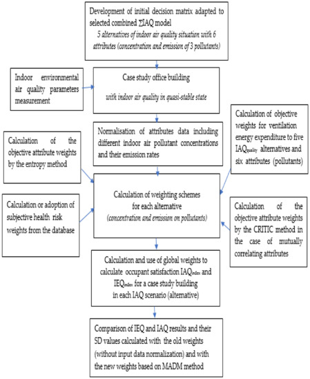
Figure 3.
The research phases to calculate the global weights for the ΣIAQ model (based on the case study building).
2.2. MADM Method Applied to the ΣIAQ Model
The basis for applying the MADM method is a decision matrix, as shown in Table 1. The issue of a weighting scheme is a problem related to making decisions with several criteria, which can be analysed using the model [26]. For every type of ∑IAQ model with Equations (4), (5) or (6), the decision matrix should be created separately.

Table 1.
Decision matrix scheme in the MADM model for the concordance of economic and human comfort criteria for each ∑IAQ scheme described by Equations (4)–(6) separately with alternatives (e.g., ∑IAQcomfort scheme configurations) and with attributes (air pollution components in quasi-stable states and emissions).
In Table 1, alternatives a1, a2…a(n) for ∑IAQcomfort configurations are defined further (in Methods). Attributes X1, X2 and Xj are the indoor air pollution concentrations of CO2, HCHO, TVOC and VOCodorous in a quasi-stable state of the indoor environment. X5(e), X6(e) and X7(e) are indoor emission processes and their rates per emission surface of CO2(e), HCH(e), introduced by an thropogenicemissions or directly emitted from construction products. In the decision matrix of the IAQ weighting scheme according to Table 1, the flow chart presented in Figure 3 provides the necessary steps and, therefore, includes MADM elements:
(1) attributes in the number j = 1 … 3 …, which are indoor air pollution concentrations covered by the models ∑IAQquality, ∑IAQcomfort and ∑IAQcomfort / health described by Equations (4)–(6) and Figure 2; however, the number of attributes beyond j = 7 (e.g., for ∑IAQcomfort/health) is not limited because model components like VOCodorous or VOCnon-odorous and other pollutants can be multiplied.
(2) alternatives i = 1 … n, which are the ∑IAQ models described by Equations (4)–(6) and Figure 2 assigned to the quasi-stable state, or defined by emissions. The selected decision model alternatives correspond to three combined indoor air quality models in various attribute set configurations (i.e., changes in attribute sets, IAQ sub-models). Alternative models, i.e.,IAQcomfort and IAQcomfort/health models, have more attributes than the IAQquality model; moreover, the number of these attributes is variable in both the pollutant and emission groups. In the group of alternatives, IAQ model systems not disturbed by emissions, e.g., IAQquality, and models distorted by emission attributes, (e) for example, were considered. The number of alternatives (Table 1) cannot be too small because the standard deviations for the set of alternatives assigned to a given attribute are calculated (i.e., for the attribute column in the decision matrix).
The assumptions in the decision model are adequate for the task of measuring the indoor air ventilation rate to obtain the assumed air quality, setting IAQ model alternatives so they meet the criteria and taking into account their importance ranking and possibility for ongoing diagnosis of alternatives to the assumed overall IEQ assessment. The model should provide a set of attributes that are important for maintaining hygienic and efficient ventilation, both of which are connected to variable air pollutants. This is important because the decisions relate to the scope of complex indoor air quality models, while planning the ventilation system depends on the amount of “excess air pollution” including VOC and SVOC compounds.
In the Materials and Methods and Results sections, an example of the implemented IAQquality model is provided, as well as a shortened Table 5 decision matrix with a set of attributes of type (e) (emission), which includes additional sources of bio-emissions (CO2 emissions), emission sources from additional equipment and finishing products (HCHO emissions), and emissions from building materials (TVOC). The choice of the attributes was facilitated by the fact that the effects of air pollution, in another open environment and system of conditions and tasks, on the economy were provided by Wang et al., 2017 [6]. This team built a Smart MCDM decision model to study the impact of outdoor air pollution on the economic development of selected zones in China. In addition, looking at the goal of the present paper to rank the importance of selection parameters for human comfort, insights could be derived from already established research procedures for the selection of construction materials [12] or waste disposal (Savic [27]). Therefore, the attributes of the decision matrix (Table 1 and Table 2) include the most typical and expected air pollutants belonging to successively developed ΣIAQ systems. The selection of attributes, i.e., types of pollution, consistent with Equations (4)–(6) also corresponds to the choice of Air Quality Index (AQI) [28].
Table 2.
Decision matrices for three ∑IAQ models with attribute data.
2.3. Flow Chart of Weighting Scheme Determination
In the analysed IAQ model, the authors considered excess concentrations that can be measured in a quasi-steady state, and emissions from additional and sometimes temporary sources that periodically increase in the ΣIAQ system of excess concentrations. The number of pollution type attributes is as strictly defined as the ΣIAQ specified composition. The number of emission type attributes is variable, adapted to the selected set of decision pollutants, and does not usually exceed the number of pollution type attributes.
The process of determining the weight for the IAQindex model, seen in a number of variants of the composition of its sub-indexes, i.e., in various alternatives, involves weighting scheme calculations adequate to the level of a particular alternative. Each weighting scheme contains relative values of global weights. These weights represent the energy expenditure of the ventilation system on the elimination of excess concentration of a given pollutant (excess concentration (2) [4]) in ventilated air. The process for determining the weighting scheme for the ΣIAQ model is shown in the flow chart in Figure 4. It should be noted that the authors considered it appropriate, after specifying the technical conditions and physics of the building for which the decision model is used, to add the costs of ventilating the anticipated excess pollutant concentrations. Based on the literature of this multi-parameter problem, however, the authors found it advisable not to insert this attribute at the current level of the generalized decision model for selecting the ΣIAQ weighting scheme.
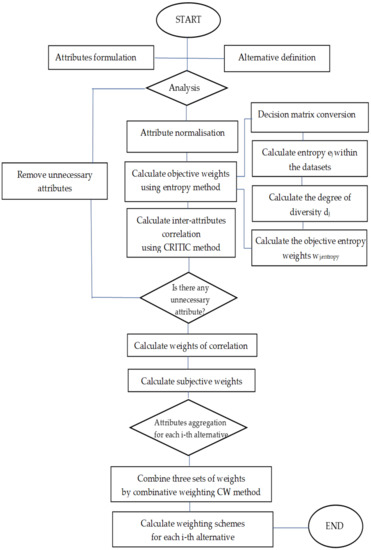
Figure 4.
Chart for subjective and objective weight determinations for the combined ∑IAQ model.
The idea of the correlation effect on weight wj,CRITIC stems from the fact that when the criteria correlation with other attributes is significant, it should have lower importance due to the roles of other criteria. An increase in the value of the concentration of a given indoor air pollutant, with a sudden (dramatic) increase in emissions, is accompanied by an increase in global weight because it must include an additional component, which is the correlation weight.
2.4. General Principles of Estimating IAQ Model Weighting Schemes
In this section, the authors provide a method with a step-by-step procedure for setting priorities in the group of dominant indoor air pollutants, considering technical, economic and health aspects, by global weights for each component of the IAQ model. Developed for the ΣIAQquality model, the MADM decision matrix includes six attributes: carbon dioxide, total VOC (TVOC) and formaldehyde concentrations (HCHO) in the indoor environment as well as additional carbon dioxide bio-emissions and total VOCs and formaldehyde emissions. All six attributes are associated with cost criteria, and in future the decision model can be developed along this trend. The MADM decision matrix of the IAQquality model includes five alternatives (combination of various IAQquality sub-components) for defining indoor air quality in a building. The informationcontained in every attribute is related to the contrast of each criterion. Standard deviation (SD) and entropy are the measures of intensity and ways to present objective criteria weights. In order to calculate the weights of criteria, the authors use objective methods: entropy and CRITIC, presented in Figure 3 and Figure 4.
Adaptation of the IAQ model with the “new” weighting procedure based on the MDMA approach to our office building case study (see Results and Discussion) was performed mainly for illustrative purposes in the context of the presented MDMA method for IAQ model development. The authors did not focus in depth on any technical issues of the building. Other Indoor Environmental Quality (IEQ) sub-components indexes, such as thermal, acoustic and visual satisfaction (in %), are presented in a paper [5] in order to provide background to the actual research problem.
The authors present the order of steps and mathematical operations leading to the determination of weighting schemes of ΣIAQ models (4), (5) and (6) separately. All model decision matrix variants are covered inan overview (Table 2), which presents decision matrices for the three types of IAQ models: ΣIAQquality, ΣIAQcomfort and ΣIAQcomfort/health, covering various types of contaminants.
The first step for estimating the MADM framework is normalisation of data (henceforth, the decision matrix indicators), which belong to different types and have different excess concentrations of the most important air pollutants and VOC emissions affecting IAQ indoor environments. In an indoor quasi stable state, attribute parameters include the concentration of these pollutants and additional increases in their concentration when the level is disturbed by additional sources of their emission or bio-pollutant emissions (1). Normalisation of attributes in various units (values of pollutant concentration and emission rate) in large ranges (attribute) is performed to obtain dimensionless quantities. Attribute normalisation is possible in several ways; however, for the research problem discussed here, the most common methods are as follows:
(a) Linear normalisation of attributes belonging to the decision matrix carried out according to the pattern of elements in the normalised decision matrix, belonging to the set of “cost attributes” according to Equation (8):
where j ∊ Nc and Nc represents a set of criteria or attributes. The minimum value of the indicator xij of the decision matrix, i.e., the normalisation of attributes in the form of the levels of air pollutants or their emissions in the decision matrix of a complex IAQ model, can be more conveniently determined using Equation (9) provided by Körth [29]:
if air pollution is a negative value indicator.
nij = min (xij)/xij
(b) Normalisation of attributes according to Wang’s scheme [6] already applied in relation to the description of air pollution. In addition, positive and negative indicator values represent different meanings (10) and (11). Air pollution is a negative value indicator (negative values), while profit from the absence of pollutants would be a positive indicator. Similarly, the values of the emission rate of individual pollutants are also negative indicators, which can be read from the emission curves, both max (xij) and min (xij) values. Therefore, in order to normalise the attributes, the authors chose negative values according to Equation (10). Positive values (type benefit) are
Negative values (type costs) are
where xij represents the original value and nij represents the value after normalisation. However, this way of normalising the IAQ decision matrix in the actual system of its application, in which some configurations (alternatives) have some attributes values equal to 0, proved to be impracticable. The same group also uses the transformer version of Equation (10) provided by Zavadskas [30] and Vujcic [31]:
The stage of data normalisation of the decision matrix is carried out after it is built, and at the same time, the max (xij) and min (xij) values are determined in the attribute columns j. These max and min values of the xij indicators are inserted into the formula for normalisation of the input data. Therefore, prior to data normalisation, the maximum and minimum values xij adopted for the attributes in the studied conditions of the IAQ model should be compiled from the literature. These values will be used to test the normalisation of the input dataset adopted in the decision matrix, while the test normalisation will also address the question of whether a given normalisation method (formulas) normalises the input dataset correctly (the normalisation result cannot be negative) [31] and whether the set of alternatives (combinations of attributes) in the decision matrix has been determined correctly. Literature [2,5,7,32,33,34,35,36,37,38,39,40] on the minimum pollutant values (min xij) include the long-term concentrations [32] or cLCI concentration values. The maximum values [2,7,36,37,38] of the max (xij) pollutant concentrations are either short-term values or allowable concentration values cELV [32] according to EN 16798-1: 2019, World Health Organization WHO guidelines [33] and EU recommendations [34]. The results of maximum and minimum concentration tests in representative groups of UK, Danish and Polish building tests published by Shrubsole [2] and Johnston [35] were used. Attributes are initially normalised assuming that, for attributes X1 … m, the values from Table 3 can be inserted into Equations (9) and (12) to obtain normalised attributes nij.
Table 3.
Example data for the ΣIAQ model decision matrix. Attribute indices xij and normalisation results nij with two methods calculated by Equations (9) and (12), as example alternatives.
2.5. Calculation of the Objective Attribute Weights by the Entropy Method
Step 1. Normalisation of indicators
Since the analysed indicators of indoor air contamination may be provided in different units, authors normalised them as a first step. Normalised decisions, however, depend on the attribute’s nature. In the entropy weights procedure, all attributes must be beneficial (positive values), but in the decision matrix all attributes are of a non-beneficial type. Therefore, the conversion of normalised indicators of “cost” type into indicators of “profit” requires building a matrix of “profit type”. As such, the higher their indicator values are, the higher the assessment of the decision variant will be. The indicators for which the criteria are based on the assessment of current air pollutants, and the assessment of the emission rate belong to the cost type indicators, are designated by non-beneficial or cost sets. In order to determine weights using the Shannon entropy method, a specific data normalisation method is used [20]. We built a matrix Y = (yij), in which all criteria will be of “profit type”. Then, the elements of the matrix are determined from Equation (13):
yij = 1/xij
The normalised decision matrix Z = [zij]n×m with the elements zij for determining entropy weights is determined with Equation (14):
for various alternatives (more or less complex indoor air quality models) and their respective attribute sets (selected IAQ sub-models to assess various pollutants and emission rates).
Step 2. Calculation of the entropy measure
The entropy vector ej for a given attribute j from the sum of components zij and ln(zij) calculated for all alternatives i = 1 … n is determined as
where zij∙lnzij is equal to 0 for zij = 0 and the variation(divergence) level vector dj calculated for each attribute as
dj = 1 − ej
Step 3. Defining the objective weight of each j as follows, based on the entropy concept
2.6. Calculation of Subjective Attribute Weights Depending on the Toxicity of Air Pollution to Humans
The weights of IAQindex models must also contain, in addition to the objective entropy weights, the subjective attribute weights that describe factors related to health human toxicity from indoor air pollution.
Variant 1. Sjhealth subjective weights from databases for criteria of “air pollution specified chemical compound” with tested chemical properties, toxicity, and “health level” and “health scores” assigned to air concentrations of this compound are treated as reference data taken directly from the literature [36] and [40,41,42,43,44]. For example, Yuan [40] adopted the following weights for selected pollutants as part of the research program:“French permanent survey on Indoor Air Quality” [43], US-EPA and WHO databases (Table 4).In some cases when detectinga larger number of indoor air contamination compounds with air concentration >5 μg/m3, additive health effects are assumed, and the subjective weight Sjhealth can be created with the EU-LCI approach.
Table 4.
Subjective weights of ten pollutants (plus hot and humid air enthalpy).
Variant 2. The subjective sjhealth weights determined by health experts depend on the toxicity of pollutants based on a number of expert opinions r greater than the number of experts k. In the case of not listing compounds in databases, the relative value (signification) of the sjhealth weight for the jth criterion (with a total number of m criteria) can be calculated by the SWARA method presented by Kersuliene et al. [45] and Zavadskas [46] using weight estimation procedures in several steps as follows.
Step 1. The relative importance of the criterion is determined by reference to the weight of sj and the weight of the previous criterion sj-1. Then, the weights of sjhealth based on the opinions of all experts are calculated. An example of a simple algorithm for determining the average subjective weight of attributes sj is based on the average of opinions (weight proposals) of attributes collected from k experts, i.e., from the formulas given by [46]. The average value of expert attribute reviews is calculated using Equation(18):
where tjk is the ranking of attribute j according to respondent k, and r is the number of respondents.
Step 2. The subjective weights can be adjusted by dividing the average values of each attribute by the sum of the average values of the attributes (19):
Step 3. Having determined the average values of attribute reviews from Equation (18) and knowing the established ranking of these opinions, you can calculate the standard deviation of attribute j in the ranking of opinions (“dispersion of expert ranking values”) by Equation (20):
Value σj2 is useful for calculating the weights of the effects of attribute correlation wj,CRITIC formula.
2.7. Calculation of the Objective Weights of Correlation between Attributes by the CRITIC Method
Use of the CRITIC (Criteria Importance Through Inter-criteria Correlation) method in the case of mutually correlating attributes (e.g., attributes constituting “quasi-fixed” impurities and attributes constituting their emissions) to estimate the correlation weights between the criteria is justified. Additionaly to the intensity contrast of dataset attributes in the decision matrix, there was another concept more recently taken into consideration by researchers using MCDM. Diakoulaki’s team [47] found that the greater the level of inter-dependency between attributes, the higher the error ranking outcome. CRITIC was analysed in [47] as an objective and new weighting system that took into consideration criteria correlations. The approach included contrast intensities (by means of SD criteria) and combined them with correlations weights. All material selection studies assume that the criteria are independent of each other, while they are also likely to influence each other. Some approaches proposed in recent years for weighting criteria when choosing material not only bypassed this approach, but they did not take into account the interdependence of criteria and proposed methods of objective weighting, which have relevant shortcomings. When correlation between criteria is suspected, the validity of the criteria can be adjusted by entering correlation weights. Calculating the weights of correlations between the criteria of a decision model using Pearson’s correlation coefficients is recommended [9,11]. The CRITIC weights marked wj,CRITIC specify a correlation between the criteria, which can include all criteria (or attributes) or only criteria that are influenced. The CRITIC method by Diakoulaki [47], Jahan et al. [12] and Ardakani et al. [10] includes estimations of differences in the “intensity” of criteria values (expressed by the value of their standard deviations) and combines them with weights based on correlation coefficients (step 4). Alternatively, the modified model in Jahan [12] uses only Pearson’s correlation coefficients and does not include standard deviation criteria in the equations. As justification, it was stated that the differences resulting from changes in the “intensity” of the criteria were already taken into account by the entropy method, and the correlation weights were calculated accordingly. Therefore, the values of the correlation weights between the criteria are calculated by [10,12] using the values of Pearson coefficients Rjk, which represent the correlation between the two selected criteria j and k (correlated criteria) and which can be calculated easily, even in MS Excel. Rjk values are read from the symmetrical linear criteria correlation matrix or calculated from Equation (21):
where xij and xik are n total number of alternatives (alternative IAQ models) and matrix elements (Table 1) xij (with a peak) of average values of the j criterion and xij of average values of k criteria (emission criteria k1..3 correlating with other criteria, e.g., emission rate of pollutants, which include selected criteria pollutant concentrations). If Rjk is close to +1 or −1, this means that the criterion is correlated highly, while Rjk close to 0 means there is no correlation. Then, the correlation weights are calculated by the CRITIC method using Rjk determined by Equation (21). The effects of the correlation impact of all criteria on other criteria can be calcualted, or the impact of selected k criteria (e.g., emissions) on related criteria of the decision model j (e.g., polluting emissions), and only then are selected correlation coefficients used. A common form of the formula for correlation weights using the CRITIC method is Equation (22) [10]:
where β is equal to +1 if two objective criteria are of the same type (either greater is better) or β = −1 otherwise. In Equation (22), Equation (23) denotes a conflict of measure created by criterion k in relation to the decision:
According to Zawadskas [30], the sum (23) ought to be multiplied by σj−, - the standard deviation (SD) of the jth criterion. The inclusion of SD follows a similar approach to the entropy approach, assigning a weight to the attribute if it has a corresponding attribute value across alternatives. A “symmetrical matrix” is developed with dimensions n × m and a generic element Rjk. The higher the divergence in the scores of alternatives in criteria j and k, the lower the value of Rjk. This step determines the conflict and then the weight of each decision criterion. The sum provided below denotes the measure of conflict created by criterion j with respect to the decision.
The modified and simplified CRITIC method, which has not been used in this study, calculates the correlation weights between criteria without calculating the symmetric linear correlation matrix Rij. The method determines the objective weights wj,CRITIC on a different principle. It determines the objective weights of the attributes by using contrast intensities for each measure, considered as SD, conflict and correlation coefficient between criteria by Zavadsas et al. [30], Vujicic et al. [31] and Adali et al. [48].
Step 1. Calculation of the normalised decision matrix for wj,CRITIC
For each criterion xij, function rij which transforms all the values of criteria into the interval [0, 1], is provided:
The basis of the transformation uses the concept of an ideal point. The initial matrix is converted into generic element matrix rij. Here, it should be noted that normalisation does not take account of the type of criteria.
Step 2. Calculation of standard deviations in attribute column j for all alternatives 1 … n.
Step 3. Calculation of Cj specifying the amount of information contained in the given attribute j.
In Equation (25), SD represents the deviation of various values for a given criterion of a mean value. The information of Cj contained in criterion j is calculated by Equation (25):
where σj is the SD of the jth criterion or alternative, and the expression rjk is considered equivalent to the correlation coefficient between the two attributes: selected attribute j and correlation attribute k.
Step 4. Calculation of the weight of the correlation of the criteria correlating k with a given criterion j is carried out using Equation(26):
Calculation of correlation coefficients should not be ignored; therefore, this study adopted a modified method of data normalisation and calculation of correlation weights between attributes based on the symmetric linear correlation matrix using the full CRITIC method. Calculation of correlation weights between criteria based on the symmetric linear correlation matrix by the CRITIC method uses a modified data normalisation method. In summary, the calculations were based on the determined correlation coefficients for attribute pairs related to the same impurities wj,CRITIC by using the following steps.
Step 1. Normalisation of initial decision matrix (Table 1)
The recommended [6] equation for normalisation of the original decision matrix for cost criteria is Equation (27)
but the authors used the transformer version [32,33] in the form:
Step 2. Calculation of standard deviations in data sets assigned to attributes j from the value rij for all alternatives 1 … n.
Step 3. Calculation of symmetric linear correlation matrix Rij.
The primary matrix (Table 1) is converted to the normalized decision matrix and later to symmetric linear correlation matrix of generic Rij elements, which are Pearson’s correlation coefficients (21) determined for all pairs of normalised sets on data rij assigned to selected attributes, at all levels of alternatives n. Then, the most likely correlations corresponding to attribute pairs (e.g., concentrations and emissions of the same compound) were selected from the matrix, and weights were calculated for them wj,CRITIC. A coefficient of linear correlation between each pair of measures is estimated using the following formula that allows to quantify the conflict occurring among various criteria. It is obvious that more discordant the scores of the alternatives in both matrix vertical i and horizontal j sections, the lower the value Rij.
Step 4. Calculation of objective weights using the CRITIC method. The weight of the jth criterion is obtained using Equation (29) presented as:
where
A higher value of Cj indicates a more considerable amount of information contained in a particular criterion. Therefore, its weight is higher. The CRITIC method assigns greater weight to criteria that have high standard deviations and low correlations with other criteria. A higher Cj value means that more information can be obtained from this criterion, which increases the relative importance of the criterion for the decision problem. The study of correlation effects by the CRITIC method is carried out by calculating the weight wj,CRITIC for the j attribute that requires it due to the anticipated impact of the k attribute, e.g., when it is known that the validity of the attribute “TVOC pollution” in a “quasi-stable state” will increase under the influence of the attribute correlating with“TVOC emission”.
2.8. Calculation of the Objective Weights for Ventilation Energy Expenditure
The objective weights for ventilation energy refer to the combined ΣIAQ model described by polynomial (1), whose words have been assigned weights described by Equation (3), based on the concept of “excess concentration”, creating the energy expenditure of ventilation. These are the relative weights calculated for each alternative of the IAQ model. The values ∆cj for pollutants adopted inthe decision matrix differ by several orders. In the IAQ index model decision matrix (Table 1), it is necessary to normalise the set of values of “excess concentrations” for the first three attributes in the ΣIAQquality system described by Equation (4). The basic problem indata normalisation for determining weights wij,energy based on the concept of “excess concentration” is the selection of formulas that can be useful for this purpose. Referring to Körth et al. [29] and Vojcica [31], it seems that the following equation can be used to normalise datasets of “type cost”, which after conversion to attributes of “type profit” (or beneficial) adjust for IAQ systems corresponding to subsequent alternatives a1 to a5. Normalised values ∆cj will correspond to “energy load” weights wij,energy = nij:
Taking into account the input data of the decision model summarised in Table 1 and Table 5, a dimensionless set of values corresponding to excess concentrations according to (2), normalised for weights, is calculated for the alternatives of this model wij,energy. for non-zero attributes j = 1, 2, 3 in the form of CO2, TVOC and HCHO pollutant concentrations.
Table 5.
Initial decision matrix with the data assigned to various IAQquality component sets and action scenariospresented by individual alternatives.
2.9. Combining the Weights by Calculation of Global Weights
The global weights wij,global contain specified weight multiplication products of various types, adjusted to the sum of these products according to the widely used procedure for building weighting development. In the flow chart (Figure 3), the wj,global weights include basic entropy weights wj,entropy, subjective weights related to health human toxicity determined using “health-related” databases sjhealth and correlation weights wj,CRITIC, and ventilation energy weights wij,energy. At the same time, correlation weights occur only in those alternatives (∑IAQ systems) in which decision matrices contain correlation criteria (this criterion is “pollutant emissions” in Table 1). The weights are assigned to individual attributes j = 1 … 6 of the decision matrix, and the weighting schemes for five alternative IAQ levels i = 1 … n are composed of weights assigned to specific attributes at a given level of alternatives from a1 to a5, which are adjusted to the sum of weights at a given alternative level i. A modified integrated weighting method, presented by Deepa et al. [49] and [15], proposed an approach to combine all weights calculated using different weight assignment approaches into a single set of weights. The equation to calculate the weights of attributes in alternative levels is
where wij,global represents thecomined weights of the criteria, wg denotes the criteria weights calculated by using one of the weight calculation methods, and g = 1, 2, …, n, where n is the number of methods used.
If a decision is made to assign a given attribute to the objective weight wj,entropy and the subjective weight associated with the risk to sjhealth health, but with adjastmentto the sum of weights at a given alternative level i, then the global weight of toxic pollution is
When the alternative and the attribute are assigned the relative weight wij,energy and when the alternative indicators are compared to the attributes of type k correlating with, e.g.,“pollution emission”, then the composite weight of the attribute correlating with the attribute “emission” also includes the weight of the correlation effect wj, CRITIC and weight wj,energy for the given attribute j at the level of the i-th alternative:
The denominators of the formulas for global attribute weights j= 1 … m at alternative levels i = 1 … n are, therefore, calculated as the sum of the products of entropy weights wj,entropy multiplied by sjhealth and wj, CRITIC and other weights, e.g., wj,energy representing the importance of the attribute for the energy load.
It should be noted that the use of the ∑IAQ model (for calculating the total energy expenditure for ventilation and using the global weight value in the IEQ inEquation (7)) requires to determine the global weight values only for the attributes of “pollution concentrations” (in the case of the IAQquality model, only for j = 1, 2, 3) in the form of relative global weights adjusted at all levels. The measures of the significance of the other attributes (emissions) are determined by the CRITIC method and are given by correlation weights that additionally impact the global weights of the “concentration” attributes. Therefore, although entropic weights are calculated just like CRITIC weights for all attributes, taking advantage of the fact that they are weights characteristic for given attributes (they are weights calculated in columns j, not relative weights), they can be “selected” and adjusted in the range of attributes to calculate relative global weights for all levels of alternatives.
2.10. Characteristics of the Case Study Building
In order to determine the weights of the IAQ model, the authors present a casestudy building and use the real scenarios inindoor environment quality. Thecasestudy building is a newly built high tower office with 49 floors and a net area of 59,000 m2 made of steel and concrete materials with a heavy glass facade. The buildingis located in Warsaw. The experimental part (measurement in situ) included analysis of CO2, HCHO and VOCs indoor concentrationsin the building interiors. Provided in [5], datasets on the pollutants supported the authors’ decision matrix development including scenarios/alternatives. At the time of the test, the building was in the pre-occupancy phaseandhadempty spaces with no furniture inside. The indoor walls were plaster covered and freshly painted. Suspended ceilings were mounted, and thefloors were coveredwith a synthetic carpet. The building installationswere active during tests. The building was tested threedays after the internal work was finished. Measurements were made on the 47th floor, covering area of almost 3000 m2. The main focus was on the IAQindex for selected open spaces in which alargenumber of usershave to reside, and which represent the largest occupied floor space. ISO and CENinternational standard based analytical methods were engaged to assess“in situ”HCHO, TVOC and CO2 concentration values. Theair samples for VOCs tests were collected viaactivesampling with anelectronic mass flow controller that controlled the air flow via test probes (10 dm3/h for VOCs and 30 dm3/h for HCHO). Indoor air samples were taken from selected representative office locationsand tested later in an accredited laboratory in accordance with ISO 16000-3:2011 and ISO 16000-6:2011. VOCs were sampled on the probe tubes filled with Tenax adsorbent. Later, they were thermally desorbed using a TD-20 device (Shimadzu, Kyoto, Japan). The process of separation and analysis of VOCs was achieved with aGC/MS gas chromatograph equipped with a mass spectrometer (model GCMS-QP2010, Shimadzu, Japan). VOCs were identified by comparing the retention times of chromatographic peaks with the retention times of reference compounds, by searching the NIST mass spectral database (USA). Identified VOC compounds were quantified using a relative identification factor from standard solution calibration curves. TVOC concentration was calculated by summing identified and unidentified VOCs eluting between n-hexadecane and n-hexane.
2.11. Building-Related Research Limitations
Building-related research limitations were also recognized because the ΣIAQ model and provided weighting scheme applied mainly to office buildings with mechanical ventilation. Quasi-static indoor environment conditions and full air mixing in the building wereassumed by the authors (perfect mix of indoor air). The IAQ model is based on sensory curves that were created by examining people’s response to a stimulus with analmost neutral influence of other indoor environment factors. This means that the applicability of the presented IAQ model is limited to indoor thermal conditions in the range of 20–26 °C and relative humidity of 30–70%. The valid clothing level of occupants was 0.5–0.8 clo, and metabolic rate accepted was 1–1.2 m. The number of air pollutants as sub-components in the IAQ model was limited to the sub-models presented in [4]. In the example case study building, we analysed building pollution situations based on sixattributes from which we built alternative situations (a1–a5) for the building. These attributes are mostcommonly used in commercial environmental building assessment systems like BREEAM or LEED. The range of applicability of the developed weighing system wasvalid up to the maximum pollution values: 1800 mg/m3 for ∆CO2, 1000 µg/m3 for TVOC and 160 µg/m3 for HCHO.
Health risk in the context of human exposure to a given pollutant is an issue usually analysed inoccupational medicine research. In this context, we consciously limited our research scope and didnot focus directly on human health risk.
3. Development of ΣIAQquality Model Weighting Schemes for the Case Study Building
3.1. Development of the Initial Decision Matrix Adapted to the Combined ∑IAQquality Model
This section providesastep-by-step approach for a numerical calculation of combined ∑IAQquality model sub-element weights presented in the example case study building.
The results of the casestudy building identified pollutants [5] and were the basis inbuilding a decision matrix. Table 5 represents the initial decision matrix (the input data table) for the defined scenario (fitting of the weighting schemes to various IAQquality quasi-stable states). The matrix consisted of six attributes (concentrations and emissions of three indoor air pollutions) and five alternatives, where:
a1—alternative based on the case study specifics presented in a previous report in [4,5]. In the building under investigation, with quasi-stable air quality, for the indoor pollutant concentrations of CO2, TVOC and HCHO, the assumption was made that the additional emissions of these three air pollutants were not measurable;
a2—alternative based on the assumption of minimum air pollution concentration levels changing very little because the emissions rate atthe minimum level does not affect the quasi-stable state of IAQ; for the CO2 bio-pollution rate and the CO2 concentration minimum level value, the bio-effluents rate from a single person during one hour was accepted [42];
a3—alternative predicting the measured air pollution quasi-stable concentration at aminimum level, but under the influence of CO2(e), TVOC (e) and HCHO (e) emission rates, it did so at a higher level (addition under minimum level waswithin the 0.25 measuring range); the TVOC or HCHO minimum levels of emission rates were calculated as 0.25 of the (max–min) range estimated by the literature on thepollution emission rate;
a4—alternative is similar to a3, but the higher influence of the emission rate of CO2(e) does not exist (there is no addition under the minimum level of CO2 emission rate);
a5—alternative is similar to a3, but the higher influence of emission ratesof TVOC and HCHO does not exist (there is no addition under the minimum level of TVOC and HCHO emission rates).
The set of alternatives is used for checking how the weighting scheme changes when the emission rate of a particular air pollutant is absent or increasing.
Simultaneously, the authors calculated all weights for the additional alternative version a2-2, which differs from alternative a2. This is based on the assumption of air pollution concentration levels, taken from the case study, practically not changing the quasi-stable state because the emissions rate is at a minimum level, like in alternative a2. A minimum level for the CO2 bio-pollution rate, and TVOC (e) and HCHO (e) minimum level emission rates were established. It can, therefore, be argued that the weighting scheme for the IEQ model with the a2-2 alternative will have a screen emission (more probable than for the a2 alternative). The decision model and its weighting schemes with alternative a2-2 and the same set of attributes havedifferent structures than alternative a2. However, as the values of indoor pollution concentrations are the same in this study (with the assumption of minimum levels of emissions alone), version a2-2 can be used for comparingthe impact of the two alternatives a2 and a2-2. Maximum xij levels of ventilation load are based on the research [2,7,32,35,38,42] and Minimum xij levels by [2,35,38,39,42].
3.2. Attribute Weights Obtained by the Entropy Method
Determination of objective attribute weights (only for attributes 1, 2 and 3, named “pollution concentration” sub-indices in IAQquality) from Equation (4), calculated in attribute columns by all levels of alternatives belonging to the decision matrix in accordance to the entropy approach, is based onuncertain information measurements contained in the decision matrix and directly provides a set of weights for criteriabased on mutual individual criteria values contrastedwithvariants for each criterionalone and then for all criteria at the same moment. The following steps are suggested in this direction.
Step 1. Normalisation of indicators for the entropy method—since the indicators of air pollutants are in different units, and since the attributes are of a non-beneficial type, the most recommended method to normalise them is used first. In particular, the transformation method according to Equation (34) solves this issue:
Table A1 (in Appendix A) presents the normalised decision matrix (according to Equation (35)) with dimensionless numbers zj representing the normalised response of alternative i on attribute j. The structure of the decision matrix contains the input parameters of atribute j = 1, 2, 3 determined on the assumption of an indoor quasi-stable state environment with minimum level of air pollution concentration and minimum emission rates.
Table 6a presents the shortage of normalised decision matrices (according to Equation (35)). The structure of alternative a2-2 (presented in Table 6b) contains the input parameters of atribute j = 1, 2, 3 based on the current experiment [5] with the assumption of an indoor quasi-stable state environment with the experimentaly determined level of air pollution concentration and with minimum emission rates.
Table 6.
Normalised decision matrices with dimensionless numbers zj for (a) alternative a2 based on the minimum level of air pollution in a quasi-stable state with minimum emission rates for (b) alternative a2-2 based on air pollution values from the case study in a quasi-stable state with emissions rates at a minimum.
Step 2. The entropy measure calculation. The measure of the jth attribute under indicator i (i ranges from 1 to n) is calculated using the following Equation (36):
where constant k = 1/ln n guarantes that ej (j = 1, 2 …, n ) belongs to the interval [0;1]. A constant k in the matrix with five alternatives can be calculated by Equation (37):
Therefore, it is possible to calculate the value of k for all attributes j = 1…6 and alternatives n = 5. With the help of Table 6a,b, it was possible to calculate ej, dj and entropy weights of criteria values wj,entropy, which are presented for Variant 1with alternative a2 and Variant 2 with a2-2 in Table 7. The degree of divergence (dj), where dj (j = 1, 2…, m), is the inherent intensity of criteria contrast Cj. The value (dj) of the average intrinsic information contained in each criterion is calculated as Equation (38):
dj = 1 − ej
Table 7.
Entropy, degree of divergence and the relative weights of attribute j.
Step 3. Calulation of the entropy weights of attributes
Next, the entropy weights of each j are calculated as follows. The final criteria weight, in the third step of the approach, may be calculated by an additive normalisation (39):
wj,entropy = (dj)/∑ (dj)
Table 7 presents the results of calculations using Equations (38) and (39).
3.3. Attribute Weights by the CRITIC Method
Step 1. Normalisation of indicators for the CRITIC method
For each criterionj and indicator xij, membership function rij, which transforms the values of attributes into the interval [0,1], is provided(40):
and the transformer version of formulas is [30,31]:
The transformation considers the concept of an ideal point. With Equation (41), the initial matrix is converted into the normalised decision matrix with the generic elements rij (Table 8a and Table 8b).
Table 8.
Normalised decision matrices. (a) (with alternative a2) based on minimum air pollution levels in a quasi-stable state with minimum emission rates; with zero-dimensional generic elements rij. (b) (with alternative a2-2) based on air pollution test study levels in a quasi-stable state with minimum emission ratesand zero-dimensional generic elements rij.
Table A2 (located in Appendix A) presents the normalised decision matrix Equation (35) with dimensionless indicators rij representing the normalised response of alternative i on attribute j.
Step 2. Calculation of symmetric linear correlation matrix Rjk based on all indicators of normalised decision matrices (Table 9) and shortages of symmetric linear correlation matrices Rjk with alternatives a2 (Table 9a) and a2-2 (Table 9b).
Table 9.
Symmetric linear correlation matrix Rij (with alternative a2) calculated for all correlation possibilities. (a) Shortage of symmetric linear correlation matrix Rij (with alternative a2) calculated for all correlation possibilities (in this shape of the matrix, it can be assumed that only six attributes are burdened with additional correlation weights, but in the recognised attribute set only the first three will be used). (b) Shortage of symmetric linear correlation matrix Rij (with alternative a2-2) calculated for all correlation possibilities.
Step 3. Determining criteria weights for “pollutant concentration” attributes using the CRITIC method.
The amount of information necessary to calculate Cj(42) includes measures of conflict Cj determined with Equations (30) or (42). Attribute (criteria) weights wj,CRITIC were obtained from Equation (43) (Table 10).
Table 10.
Results of the CRITIC method application for decision matrix with alternatives a2 and a2-2.
Aconflict measure created by criterion j due to the decision defined by the rest of the criteria can be calcualted, which determinesa quantity of the information in relation to each criterion:
Objective CRITIC criteria weights for a chosen attribute are obtained by normalising (adjusting) the values of Cj and, in particular, alternative levels (43):
3.4. Relative Weights Obtained by Normalisation of the “Excess Concentration”
Taking into account the input data of the decision model compiled in the input decision matrix with alternatives (Table 5), alternatives a1 to a5 (with values of excess concentrations ∆cj according to (2) [4]) were calculated with weights wij,energy for non-zero attributes j = 1, 2, 3. In order to determine the “energy load” weight, the following steps are recommended.
Step 1. Assuming that the minimum concentration value cref in the definition of “excess concentration” given in Equation (2) may be the minimum value min (xij), then the formula for normalisation (43) can be determined, based on the data for the alternative a1 obtained in real case studies [5] and data from the literature [2,51,52] regarding the minimum values of pollutants (TVOC and HCHO) occurring in a building. Justification for the manner of assuming the minimum and maximum values of pollution in a building with CO2 bio-pollution is discussed in the notes of Table 5.
Step 2. Normalisation of weights (energy load) wij,energy using Equation (9) transformed to (44) for attributes of type “cost”. According to [29,31], it seems that the equation can be used to normalise non-beneficial datasets, which after conversion to profit (or beneficial) attributes can be adjusted for IAQ systems corresponding to subsequent alternatives from a1 to a5. Transformation of the excess concentration values, which correspond to the indicators xij at the levels of subsequent alternatives a1 to a5 taken from Table 5, gives the weight of “energy load”wij, energy:
Normalisation of weights based on the concept of “excess concentration”— correct applicationof weights of Equation (44) is possible on the assumption that the min (xij) value of indoor pollution determined on the basis of insitu measurements and given in the input decision matrix (Table 5) corresponds to the standard value cref from Equations (2) and (3).
Step 3. Calculation of the relative values of “energy load” weights assigned to attributes of CO2, TVOC and HCHO pollutant indoor concentrations (Table 11).
Table 11.
Normalisation of the energy load relative weights calculated with Equation (44).
4. Results
4.1. Global Weights Calculated for the IAQquality Model Alternatives
The final step of the weight development methodin Section 3 is to aggregate the calculated set of “component” weights and obtain the resultant global weights. Table 12 shows the determination of global weights calculated according to Equation (33), when the attributes do not take part in the emission process (attribute type j),and Equation (34) when attributesdo take part in the emission process (attribute type k). Weight values adequate for the numerical example are taken for the set of alternatives a2and a2-2.
Table 12.
Relative global weights in the weighting schemes calculated for five alternatives of the IAQ model (a1 to a5); global weights obtained with Equation (32).
4.2. The Results of the New Weighting Method Applied on IAQindex and IEQindex Results for theCaseStudy Building
A numerical example of the combined ∑IAQquality model with the new weighting scheme, developed according to Figure 3, is presented in Table 13 in the context of the overall Indoor Environmental Quality (IEQ) asessement of thecasestudy office building (IEQ is the predicted percentage of users satisfied with all components of indoor environmental quality). The input indoor parameters for the case study (in order to assess IEQ sub-components) are taken from previous papers [4,5], where the measured pollutant concentrations were cCO2 = 450 ppm, cTVOC = 787 μg/m3 and cHCHO = 18 μg/m3 in the case study building a week after completion of the finishing works.
Table 13.
The physical parameters representing the indoor environment of the case study and the IEQindex results calculated from Equation (7) with sub-component ∑IAQ calculations (old approach and new); assuming realistic uncertainty of measurements for a case study (old and new weight systems applied and compared).
The uncertainty of user dissatisfaction with pollutant concentration is determined by a combination of two groups of components. The first measurement uncertainty is related to the real uncertainty of parameters biases when there are measured in indoor environments. The second group concerns the uncertainty of votes in the sensory tests (reliability of responses to a given stimulus of the indoor environment are discussed in literature). In practice, a metrological analysis of the IEQ model (where ∑IAQ index is the sub-model) was provided in our previous paper [8] considering provisions of the international metrological guideline: ISO BIPM JCGM 100:2009 Guide to the expression of uncertainty in measurement. For all other possible scenarios, the uncertainty for determining the ∑IAQ index would be up to ±10% to ±30% (depending on each pollution model uncertainty assessment and the number of IAQ model components taken into account).
5. Discussion
5.1. New Weighting Method Applied on IAQindex and IEQindex Estimation for a CaseStudy Building and Comparison of Its Results with Old Crude Weighting SystemResults
The previous approach by their weighting scheme (Table 13) was based on the treatment of all main pollutantsin ununiform way. The weights were previously set as equal (for pollutants with disproportionately different concentrations) or as dependent only on the energy expenditure on ventilation (for pollutants with similar) concentrations. The new IAQ and IEQ index results based on MDMA-developed weights werecompared to the old method. The system of objectified weights used for a numerical example of IAQ and IEQ building assessment leads to important conclusions. As expected, the use of objectified weights means that the results of the IAQ and IEQ indices weredifferent than those with subjective weights. For example, at low CO2 indoorconcentrations, the role of this parameter in the IAQindex assessment was overstated. This is the case for most BMS systems controlling building ventilation, where currently the number of air exchanges (ACH) depends mainly on CO2 concentration measurements. At relatively low CO2 air concentrations <1500 ppm, the CO2 priority compared to HCHO or TVOC attributes is much lower. The cumulative weight of the HCHO and TVOC arguments compared to the “old” IAQ calculation method increased by 48%. This is important from the point of view of planning and managing ventilation systems. According to calculations, the number of users satisfied with the level of CO2 (85% satisfied) wasa good result. Nevertheless, at the same time, the theoretical number of users satisfied with TVOC concentration wasonly 52%. With novel objective weights for the TVOC argument, the number of users satisfied with IAQ will decrease. In the case of the present studyand the new weight system, the value of IAQindex decreased about 10% compared to previous calculations using the old method. Further, if one considers the existence of additional emissions from the building, finishing materials and furniture, the value of satisfied users will decrease by another 5.5%.
The authors strongly believe that the new approach to weights gives objective and more adequate results for the IAQ and IEQ models. Wider use of the new weighting method can be effective upon supplementing databases with the subjective weights of health risks for various volatile substances in the air.
5.2. The WeightingProblem in Indoor Air Quality Component Sets Framework
The weights in any decision-making model should not be arbitrary [53]. Some researchers still use weights in modelling without justification. A solution to the weight problem in indoor air quality modelling is proposed. Global weights are not only measures of the importance of attributes in the human–indoor building environment relationship, health risks and possible disturbances of the quasi-stable state due to correlations between attributes, but they are also measures of the potential load of ventilation impacted by emissions and excess concentrations of additional costs for energy use. In this context, the adoption of objectified weights in the IAQ model (also any other model, where the proposed method can be transferred) has significant practical contribution. It is suggested, knowing the specific air pollution values (attributes) for the analyzed building, to calculate the weights for a new alternative created by the user in accordance with the method proposed in article. For less insightful research, the authors suggest using a set of weights developed by us (Table 12) for scenarios/alternatives that aremost similar to the scenario under consideration. According to the adopted MADM method for each analyzed alternative (a1–a5 scenarios for the indoor environment described by concentration/emission levels for attributes or types of pollutants adopted in the IAQ model), global weights for each attribute (CO2 or TVOC or HCHO concentration) are calculated separately as the numerical coefficients of Equations (4) or (6). Thisis because the component weights (e.g., CRITIC correlation weight) of global weights depend on the values of the attributes (air pollution concentrations and emissions). Table 12 shows the calculated global weights wij,global for each attribute for each alternative a1–a5. For alternative a1 (measured concentrations in thecase study building with an assumption of no additional emissionsform construction products and athropogenic CO2), global weights of the IAQindex model are 0.0194279 for CO2, 0.478148 for TVOC and 0.5024236 for HCHO. For alternative a2 (minimum concentration levels with minimum emission rates), global weights are 0.0466775 for CO2, 0.938422 for TVOC and 0.0149017 for HCHO. For alternative a2-2 (case study result concentrations with minimum emission rates), global weights are 0.0349865 for CO2, 0.935155 for TVOC and 0.0298593 for HCHO. For alternative a3 (minimum concentration level; (e) minimum + 25% range of emission rate), global weights are 0.0422678 for CO2, 0.9426554 for TVOC and 0.0150769 for HCHO. For alternative a4 (minimum concentration level; (e) minimum +25% range of TVOC and HCHO emission rates), global weights are 0.07795658 for CO2, 0.9075486 for TVOC and 0.014494798 for HCHO. For alternative a5 (minimum concentration level; emission minimum +25% range of CO2 emission rate), global weights are 0.0422712976 for CO2, 0.942738165 for TVOC and 0.014990546 for HCHO. The obtained global weight results clearly indicate which pollutant attributes have priority. In ranges up to about 1500 ppm CO2 in indoor air, the weight of this attribute in the IAQ model is very small. This means that the ventilation system should take into account, in this respect, the removal of excess TVOC concentration first and, in the second place, excess HCHO. For all alteratives, the weight of the TVOC attribute is significant (for a2–a5, weight is over 90%). The weights for TVOC and HCHO are significantly higher than for CO2 (one order of magnitude). A 25% increase in CO2 emissions will not increase its weight in the model.
In this article, the authors have described in detail a procedure for the subjective and objective weight determination for a combined ΣIAQ model, which is composed of the following basic steps:
- Development of an initial decision matrix adapted to the type of the combined ∑IAQ model;
- Normalisation of attribute data including different indoor air pollutant concentrations and their emission rates;
- Calculation of the objective attribute weights by the entropy method;
- Calculation or adoption of subjective health-connected weights from the database;
- Use of the CRITIC (Criteria Importance Through Inter-criteria Correlation) method in the case of mutually correlating attributes;
- Calculation of objective weights for ventilation energy expenditure to various IAQ sub-components (pollutants);
- Calculation of relative global weights for all significant air pollutants of the ∑IAQ model, considered in various schemes (various alternatives in the framework of decision model).
In our case study building (Table 13), the IAQ model determines global weight values for the attributes of “pollution concentrations” in the form of relative global weights adjusted at all alternative levels. The measures of the significance of the other attributes (additional emissions) are determined by the CRITIC method and are given by correlation weights that additionally impact the global weights of the “concentration” attributes. Therefore, although entropy weights are calculated just like CRITIC weights for all attributes, taking advantage of the fact that they are weights characteristic for given attributes, they can be “selected” and adjusted in the range of the first “concentration” attributes in order to calculate relative global weights for all levels of alternatives.
Thus, the determined global weights are valid within the IAQquality model (4) treated as a sub-expression in the IEQ equation model described by Equation (7). It seems that the approach presented in this study may easily be replicated by other similar IAQ models.
In our future research, the authors will try to unambiguously link the proposed IAQ model and weight system with the demand for ventilation air for various alternatives and the ventilation systems used in case study buildings.
6. Conclusions
Currently, the issue of comfort assessement, based on user satisfaction models, is discussed in numerous research works, but in most of them indoor comfort is analyzed in terms of thermal comfort only [54,55,56].Fortunately, the recently published european standrd EN 16798-1: 2018 [7] included a wider number of indoor comfort criteria. This standard provides an approach to the classification of IAQ and IEQ models and supportscertification of buildings taking into account specific components of the environmental comfort (IEQ sub-models) including ∑IAQ (which is also composed of sub-components in functions of pollutant concentrations). This standard and any relatedreseach does not provide practical guidance on how to combine ∑IAQ model components into one indicator that could be used to classify indoor air conditions and does not provide information of how to aggregate components by an objective weighting system.With the research challenge in mind, the authors presented a relevant IAQ model in [4].In this paper, the authors provided astep-by-step procedure for determining the combined weighting scheme for the IAQ index equation, using the MADMdecision model including calculation of the objective attribute weights by the entropy method, calculation or adoption of subjective health-connected weights from the reference database, use of the CRITIC method in the case of mutually correlating attributes and calculation of objective weights for ventilation energy expenditure to various IAQ sub-components (pollutants). The assumption of the decision model is adequate for the task of rating indoor air ventilation to determine the assumed air quality (our actual work), and setting IAQ model alternatives so that they can meet the criteria taking into account their importance ranking and possibility of ongoing diagnostics of alternatives connected to the perceived actual indoor air situation. The presented weigthing scheme approach for the IAQ model may be regarded as objective, and it generates weighted criteria values (for each analysed attribute and indoor scenario) directly from the variations in criteria values. The provided method eliminates the problems of IAQ model weights with using the subjectivepoint of viewas well as the incompetence orabsence of a responsible decision-maker. The MADM approach, as shown in thiscase study, is based on simple mathematics and can, therefore, be used effectively for choosing the best IEQ and ventilation strategies.
Author Contributions
Conceptualisation, M.P. and K.K.; methodology, M.P. and K.K.; software, M.P. and K.K.; validation, M.P. and K.K.; formal analysis, M.P.; investigationtest, resources, M.P.; data curation, M.P.; writing—Original draft preparation, M.P. and K.K.; writing—Review and editing, M.P. and K.K.; visualisation, M.P.; supervision, M.P.; project administration, M.P.; funding acquisition, M.P. Both authors have read and agreed to the published version of the manuscript.
Funding
This research did not receive external funding.
Conflicts of Interest
The authors do not declare any conflicts of interest.
Appendix A
Table A1.
Normalised decision matrix for the entropy method based on Equation (35).
Table A1.
Normalised decision matrix for the entropy method based on Equation (35).
| Alternatives | Attribute X = 1…m | |||||
|---|---|---|---|---|---|---|
| ΔCO2 | TVOC | HCHO | CO2 (e) | TVOC (e) | HCHO (e) | |
| mg/m3 | μg/m3 | μg/m3 | mg/m3∙h | μg/m3h | μg/m2h | |
|
a1 test study [5} +(e) emission rate = 0 |
810 mg/m3 1/xi = 0.0012 zij = 0.1043 |
787 μg/m3 1/x = 0.0013 zij = 0.0531 |
18 μg/m3 1/xij = 0.056 zij = 0.175 | 0 | 0 | 0 |
|
a2 minimum; (e) minimum TVOC and HCHO emission +1h; (e) minimum CO2 one person |
376.2 mg/m3 1/xij = 0.00265 zij = 0.2304 |
167.6 μg/m3 1/x = 0.0060 zij = 0.2449 |
10.6 g/m3 1/xij = 0.094 zij = 0.2937 |
16.2 mg/m3h 1/xij = 0.062 zij = 0.3333 |
13.6 μg/m3h 1/xij = 0.073 zij = 0.3201 |
4.26 μg/m2h 1/xij = 0.234 zij = 0.4134 |
|
a3 minimum+1h; (e) minimum TVOC HCHO +25% concentration range (e) minimum CO2 +25% concentration two persons2) |
392.4 mg/m3 1/x = 0.0025 zij = 0.2174 |
178.3 μg/m3 1/x = 0.0056 zij = 0.2286 |
26.0 μg/m3 1/x = 0.038 zij = 0.1187 |
32.4 mg/m3 ∙ h 1/xij = 0.031 zij = 0.1666 |
Σ
24.3 μg/m3h 1/xij = 0.041 Zij = 0.1798 |
Σ
20.2 μg/m2 h 1/xij = 0.049 zij = 0.0866 |
|
a4 minimum+1h; (e) minimum TVOC, HCHO +25% concentration range; (e) CO2 minimum one person |
376.2 mg/m3 1/x = 0.00265 zij = 0.2304 |
178.3 μg/m3 1/x = 0.0056 zij = 0.2286 |
26.0 μg/m3 1/xij = 0.038 zij = 0.1187 |
16.2 mg/m3h 1/xij = 0.062 zij = 0.3333 |
Σ
24.3 μg/m3h 1/xij = 0.041 zij = 0.1798 |
Σ
20.2 μg/m2 h 1/xij = 0.049 zij = 0.0866 |
|
a5 minimum+1h;(e) minimum TVOC, HCHO; (e) CO2 minimum + 25% concentration range; two persons |
392.4 mg/m3 1/x = 0.0025 zij = 0.2174 |
167.6 μg/m3 1/x = 0.0060 zij = 0.2449 |
10.6 g/m3 1/x = 0.094 zij = 0.2937 |
32.4 mg/m3h /xij = 0.031 zij = 0.1666 |
13.6 μg/m3h 1/xij = 0.073 zij = 0.3201 |
4.26 μg/m2h 1/xij = 0.234 zij = 0.4134 |
| ∑ 1/xij | 0.0115 | 0.0245 | 0.32 | 0.186 | 0.228 | 0.566 |
Table A2.
Normalisation of decision matrix with alternative a2 (Table 5) for the CRITIC method.
Table A2.
Normalisation of decision matrix with alternative a2 (Table 5) for the CRITIC method.
| Alternatives | Attribute X = 1…m | |||||
|---|---|---|---|---|---|---|
| ΔCO2 | TVOC | HCHO | CO2(e) | TVOC (e) | HCHO (e) | |
| mg/m3 | μg/m3 | μg/m3 | mg/m3∙h | μg/m3h | μg/m2h | |
| a1 Test report [5]; +(e) emission rate = 0 |
810 mg/m3 810–810/ −433.8 = 0 |
787 μg/m3 787–787/ −619.4 = 0 |
18μg/m3 18–26/ −15.4 = 0.519 |
0 0–32.4/ −32.4 = 1 |
0 0–24.3/ −24.3 = 1 |
0 0–20.2/ −20.2 = 1 |
| a2 minimum; (e) minimum TVOC, HCHO +1h; (e) minimum CO2 one person |
376.2 mg/m3 376.2–810/ −433.8 = 1 |
167.6 μg/m3 167.6–787/ −629.4 = 1 |
10.6 μg/m3 10.6–26/ −15.4 = 1 |
16.2 mg/m3h 16.2–32.4/ −32.4 = 0.5 |
13.6 μg/m3h 13.6–24.3/ −24.3 = 0.440 |
4.26 μg/m2h 4.26–20.2/ −20.2 = 0.789 |
|
a2-2 Test study [5]; CO2 TVOC, HCHO; (e) minimum emission rate; (e) CO2 one person |
810 mg/m3 810–810/ −433.8 = 0 |
787 μg/m3 787–787/ −619.4 = 0 |
18 μg/m3 18–26/ −15.4 = 0.519 |
16.2 mg/m3h 16.2–32.4/ −32.4 = 0.5 |
13.6 μg/m3h 13.6–24.3/ −24.3 = 0.440 |
4.26 μg/m2h 4.26–20.2/ −20.2 = 0.789 |
| a3 minimum +1h; (e) minimum +25% TVOC, HCHO concentration range; (e) CO2 two persons |
392.4 mg/m3 392.4–810/ −433.8 = 0.963 |
178.3 μg/m3 178.3–787/ −629.4 = 0.967 |
26.0 μg/m3 26.0–26.0/ −15.4 = 0 |
32.4 mg/m3h two persons 32.4–32.4/ −32.4 = 0 |
24.3 μg/m3h 24.3–24.3/ −24.3 = 0 |
20.2 μg/m2 h 20.2–20.2/ −20.2 = 0 |
|
a4 minimum+1h; (e) minimum +25% TVOC, HCHO concentration range (e) minimum CO2 one person |
376.2 mg/m3 376.2–810/ −433.8 = 1 |
178.3 μg/m3 178.3–787/ −629.4 = 0.967 |
26.0 μg/m3 26.0–26.0/ −15.4 = 0 |
16.2 mg/m3h 16.2–32.4/ −32.4 = 0.5 |
24.3 μg/m3h 24.3–24.3/ −24.3 = 0 |
20.2 μg/m2 h 20.2–20.2/ −20.2 = 0 |
|
a5 minimum+1h; (e) minimum +25% CO2 2 persons; (e) minimum TVOC and HCHO |
392.44 mg/m3 392.4–810/ − 433.8 = 0.963 |
167.6 μg/m3 167.6–787/ −629.4 = 1 |
10.6 μg/m3 10.6–26/ −15.4 = 1 |
32.4] mg/m3h 32.4–32.4/ −32.4 = 0 |
13.6 μg/m3h 13.6–24.3/ −24.3 = 0.440 |
4.26 μg/m2h 4.26–20.2/ −20.2 = 0.789 |
| Maximum xij value of concentration range lit. | 1800 mg/m3 | 1000 μg/m3 | 160 μg/m3 |
64.8 mg/m3∙h four persons | 57.1 μg/m3h | 68.2 μg/m2h |
| Maximum xij value in j attribute column | 810 mg/m3 | 787 μg/m3 | 26.0 μg/m3 | 32.4 μg/m3 | 24.3 μg/m3h | 20.2 μg/m2h |
| Minimum xij level of ventilation load (lit.) | 360 mg/m3 | 154 μg/m3 | 5.8 μg/m3 | 16.2 mg/m3h | 13.6 μg/m3h | 4.26 μg/m2h |
| Minimum xij value in attribute j column | 376.2 | 167.6 | 10.6 | 0 | 0 | 0 |
| Minimum xij–maximum xij | −433.8 | −619.4 | −15.4 | −32.4 | −24.3 | −20.2 |
References
- Navarro, I.J.; Yepes, V.; Martí, J.V. A Review of Multicriteria Assessment Techniques Applied to Sustainable Infrastructure Design. Adv. Civ. Eng. 2019, 2019, 1–16. [Google Scholar] [CrossRef]
- Shrubsole, C.; Dimitroulopoulou, S.; Foxall, K.; Gadeberg, B.; Doutsi, A. IAQ guidelines for selected volatile organic compounds (VOCs) in the UK. Build. Environ. 2019, 165, 106382. [Google Scholar] [CrossRef]
- Piasecki, M.; Kostyrko, K.; Pykacz, S. Indoor environmental quality assessment: Part 1: Choice of the indoor environmental quality sub-component models. J. Build. Phys. 2017, 41, 264–289. [Google Scholar] [CrossRef]
- Piasecki, M.; Kostyrko, K.B. Combined model for IAQ assessment: Part 1—Morphology of the model and selection of substantial air quality impact sub-models. Appl. Sci. 2019, 9, 3918. [Google Scholar] [CrossRef]
- Piasecki, M.; Kozicki, M.; Firlag, S.; Goljan, A.; Kostyrko, K. The approach of including TVOCs concentration in the indoor environmental quality model (IEQ)—Case studies of BREEAM certified office buildings. Sustainability 2018, 10, 3902. [Google Scholar] [CrossRef]
- Wang, Q.; Dai, H.N.; Wang, H. A smart MCDM framework to evaluate the impact of air pollution on city sustainability: A case study from China. Sustainability 2017, 9, 911. [Google Scholar] [CrossRef]
- CEN. Energy Performance of Buildings—Ventilation of Buildings—Part 1: Indoor Environmental Input Parameters for Design and Assessment of Energy Performance of Buildings Addressing Indoor Air Quality, Thermal Environment, Lighting and Acoustics; EN 16798; CEN: Brussels, Belgium, 2019. [Google Scholar]
- Piasecki, M.; Kostyrko, K.B. Indoor environmental quality assessment, part 2: Model reliability analysis. J. Build. Phys. 2018, 5, 1–28. [Google Scholar] [CrossRef]
- Wong, L.T.; Mui, K.W.; Hui, P.S. A multivariate-logistic model for acceptance of indoor environmental quality (IEQ) in offices. Build.Environ. 2008, 43, 1–6. [Google Scholar] [CrossRef]
- Alemi-Ardakani, M.; Milani, A.S.; Yannacopoulos, S.; Shokouhi, G. On the effect of subjective, objective and combinative weighting in multiple criteria decision making: A case study on impact optimization of composites. Expert Syst. Appl. 2016, 46, 426–438. [Google Scholar] [CrossRef]
- Shanian, A.; Savadogo, O. A methodological concept for material selection of highly sensitive components based on multiple criteria decision analysis. Expert Syst. Appl. 2009, 36, 1362–1370. [Google Scholar] [CrossRef]
- Jahan, A.; Mustapha, F.; Sapuan, S.M.; Ismail, M.Y.; Bahraminasab, M. A framework for weighting of criteria in ranking stage of material selection process. Int. J. Adv. Manuf. Technol. 2012, 58, 411–420. [Google Scholar] [CrossRef]
- Moridi, P.; Atabi, F.; Nouri, J. Weighting and prioritizing of air pollutant filtration technologies for controlling NH3, PM and VOCs by fuzzy TOPSIS method. Iran Occup. Heal. 2015, 12, 1–9. [Google Scholar]
- Keshavarz Ghorabaee, M.; Zavadskas, E.K.; Turskis, Z.; Antucheviciene, J. A new combinative distance-based assessment (CODAS) method for multi-criteria decision-making. Econ. Comput. Econ. Cybern. Stud. Res. 2016, 50, 25–44. [Google Scholar]
- Invidiata, A.; Lavagna, M.; Ghisi, E. Selecting design strategies using multi-criteria decision making to improve the sustainability of buildings. Build. Environ. 2018, 139, 58–68. [Google Scholar] [CrossRef]
- Zavadskas, E.K.; Kaklauskas, A.; Turskis, Z.; Kalibatas, D. An approach to multi-attribute assessment of indoor environment before and after refurbishment of dwellings. J. Environ. Eng. Landsc. Manag. 2009, 17, 5–11. [Google Scholar] [CrossRef]
- Zavadskas, E.K.; Cavallaro, F.; Podvezko, V.; Ubarte, I.; Kaklauskas, A. MCDM assessment of a healthy and safe built environment according to sustainable development principles: A practical neighborhood approach in vilnius. Sustainability 2017, 9, 702. [Google Scholar] [CrossRef]
- Noryani, M.; Sapuan, S.M.; Mastura, M.T. Multi-criteria decision-making tools for material selection of natural fibre composites: A review. J. Mech. Eng. Sci. 2018, 12, 3330–3353. [Google Scholar] [CrossRef]
- Issa, U.H.; Miky, Y.H.; Abdel-Malak, F.F. A decision support model for civil engineering projects based on multi-criteria and various data. J. Civ. Eng. Manag. 2019, 25, 100–113. [Google Scholar] [CrossRef]
- Lotfi, F.H.; Fallahnejad, R. Imprecise shannon’s entropy and multi attribute decision making. Entropy 2010, 12, 53–62. [Google Scholar] [CrossRef]
- Peng, A.H.; Xiao, X.M. Material selection using PROMETHEE combined with analytic network process under hybrid environment. Mater. Des. 2013, 47, 643–652. [Google Scholar] [CrossRef]
- Huang, I.B.; Keisler, J.; Linkov, I. Multi-criteria decision analysis in environmental sciences: Ten years of applications and trends. Sci. Total Environ. 2011, 19, 3578–3594. [Google Scholar] [CrossRef]
- Cegan, J.C.; Filion, A.M.; Keisler, J.M.; Linkov, I. Trends and applications of multi-criteria decision analysis in environmental sciences: Literature review. Environ. Syst. Decis. 2017, 37, 123–133. [Google Scholar] [CrossRef]
- Brauers, W.K.M.; Zavadskas, E.K. Robustness of MULTIMOORA: A method for multi-objective optimization. Informatica 2012, 23, 1–25. [Google Scholar] [CrossRef]
- Hafezalkotob, A.; Hafezalkotob, A. Extended MULTIMOORA method based on Shannon entropy weight for materials selection. J. Ind. Eng. Int. 2015, 12, 1–13. [Google Scholar] [CrossRef]
- Xu, Z. Uncertain Multi-Attribute Decision Making: Methods and Applications; Springer: Berlin/Heidelberg, Germany, 2015; ISBN 9783662456408. [Google Scholar]
- Jovanovic, S.; Savic, S.; Jovicic, N.; Boskovic, G.; Djordjevic, Z. Using multi-criteria decision making for selection of the optimal strategy for municipal solid waste management. Waste Manag. Res. 2016, 34, 884–895. [Google Scholar] [CrossRef] [PubMed]
- Mintz, D. Technical Assistance Document for the Reporting of Daily Air Quality—The Air Quality Index (AQI); EPA 454/B12-001; U.S. Environmental Protection Agency, Office of Air Quality Planning and Standards, Air Quality Assessment Division: Research Triangle Park, NC, USA, 2013. [Google Scholar]
- Körth, H. Zur Berücksichtigung mehrerer Zielfunktionen bei der Optimierung von Produktionsplänen. Math. Wirtsch. 1969, 6, 184–201. [Google Scholar]
- Zavadskas, E.K.; Stević, Ž.; Turskis, Z.; Tomašević, M. A novel extended EDAS in Minkowski space (EDAS-M) method for evaluating autonomous vehicles. Stud. Inform. Control 2019, 28, 255–264. [Google Scholar] [CrossRef]
- Vujicic, M.; Papic, M.; Blagojevic, M. Comparative analysis of objective techniques for criteria weighing in two MCDM methods on example of an air conditioner selection. Tehnika 2017, 67, 422–428. [Google Scholar] [CrossRef]
- Rode, C. IEA Indoor Air Quality Design and Control in Low-Energy Residential Buildings—Annex 68—Subtask 1: Defining the Metrics. In the Search of Indices to Evaluate the Indoor Air Quality of Low-Energy Residential Buildings; AIVC Contributed Report 17; Technical University of Denmark: Copenhagen, Denmark, 2017. [Google Scholar]
- WHO Regional Office for Europe. Evolution of WHO Air Quality Guidelines: Past, Present and Future; WHO Regional Office for Europe: Copenhagen, Denmark, 2017. [Google Scholar]
- Carrer, P.; de Oliveira Fernandes, E.; Santos, H.; Hänninen, O.; Kephalopoulos, S.; Wargocki, P. On the development of health-based ventilation guidelines: Principles and framework. Int. J. Environ. Res. Public Health 2018, 15, 1360. [Google Scholar] [CrossRef] [PubMed]
- Johnston, C.J.; Andersen, R.K.; Toftum, J.; Nielsen, T.R. Effect of formaldehyde on ventilation rate and energy demand in Danish homes: Development of emission models and building performance simulation. Build. Simul. 2020, 13, 197–212. [Google Scholar] [CrossRef]
- Piasecki, M.; Kostyrko, K.; Fedorczak-Cisak, M.K.N. The Air Enthalpy as IAQ Indicator in Hot and Humid Environments—Experimental Evaluation. Energies 2020, 13, 1481. [Google Scholar] [CrossRef]
- Teleszewski, T.; Gładyszewska-Fiedoruk, K. The concentration of carbon dioxide in conference rooms: A simplified model and experimental verification. Int. J. Environ. Sci. Technol. 2019, 16, 8031–8040. [Google Scholar] [CrossRef]
- Hori, H.; Ishimatsu, S.; Fueta, Y.; Ishidao, T. Evaluation of a real-time method for monitoring volatile organic compounds in indoor air in a Japanese university. Environ. Health Prev. Med. 2013, 18, 285–292. [Google Scholar] [CrossRef] [PubMed]
- U.S. Green Building Council. USGBC LEED v4 for Building Design and Construction—Current Version; U.S. Green Building Council: New York, NY, USA, 2019. [Google Scholar]
- Yuan, J.; Han, J.H.; Xie, X.D.; Qi, Z.Y.; Yang, X.; Zhao, B.; Zhao, R.; Ye, J.J.; Xie, X.D.; Qi, Z.Y.; et al. A new indoor air quality assessment system and its software tool. In Proceedings of the Indoor Air 2005, 10th International Conferenceon Indoor Air Quality and Climate, Beijing, China, 4–9 September 2005; Volume 1–5. [Google Scholar]
- Tao, H.; Fan, Y.; Li, X.; Zhang, Z.; Hou, W. Investigation of formaldehyde and TVOC in underground malls in Xi’an, China: Concentrations, sources, and affecting factors. Build. Environ. 2015, 85, 85–93. [Google Scholar] [CrossRef]
- Ye, W.; Zhang, X.; Gao, J.; Cao, G.; Zhou, X.; Su, X. Indoor air pollutants, ventilation rate determinants and potential control strategies in Chinese dwellings: A literature review. Sci. Total Environ. 2017, 586, 696–729. [Google Scholar] [CrossRef]
- Péry, A.; Bonvallot, N.; El Yamani, M.; Boulanger, G.; Karg, F.; Mosqueron, L.; Ismert, M.; Guillossou, G.; Glorennec, P. French occupational exposure limit and toxicological reference values: Objectives and methods. Environ.Risques Sante 2013, 12, 442–449. [Google Scholar]
- Mosqueron, L.; Kirchner, S.; Nedellec, V. Bilan des études françaises sur la mesure de la qualité de l’air à l’intérieur des bâtiments (1990–2001). Environ. Risques Sante 2002, 1, 31–41. [Google Scholar]
- Keršulienė, V.; Zavadskas, E.K.; Turskis, Z. Selection of rational dispute resolution method by applying new step-wise weight assessment ratio analysis (swara). J. Bus. Econ. Manag. 2010, 21, 32–42. [Google Scholar] [CrossRef]
- Zavadskas, E.K.; Turskis, Z.; Ustinovichius, L.; Shevchenko, G. Attributes weights determining peculiarities in multiple attribute decision making methods. Eng. Econ. 2010, 21, 32–43. [Google Scholar]
- Diakoulaki, D.; Mavrotas, G.; Papayannakis, L. A multicriteria approach for evaluating the performance of industrial firms. Omega 1992, 20, 467–474. [Google Scholar] [CrossRef]
- Adalı, E.A.; Işık, A.T. Critic and Maut Methods for the Contract Manufacturer Selection Problem. Eur. J. Multidiscip. Stud. 2017, 2, 93–101. [Google Scholar] [CrossRef]
- Deepa, N.; Ganesan, K.; Srinivasan, K.; Chang, C.Y. Realizing sustainable development via modified integrated weighting MCDM model for Ranking Agrarian Dataset. Sustainability 2019, 11, 6060. [Google Scholar] [CrossRef]
- American Industrial Hygiene Association AIHA. Odor Thresholds for Chemicals with Established Health Standards; AIHA: Fairfax, VA, USA, 2013. [Google Scholar]
- Noguchi, M.; Mizukoshi, A.; Yanagisawa, Y.; Yamasaki, A. Measurements of volatile organic compounds in a newly built daycare center. Int. J. Environ. Res. Public Health 2016, 13, 736. [Google Scholar] [CrossRef] [PubMed]
- Wu, Y.; Lu, Y.; Chou, D.-C. Indoor air quality investigation of a university library based on field measurement and questionnaire survey. Int. J. Low Carbon Technol. 2018, 13, 148–160. [Google Scholar] [CrossRef]
- Fedorczak-Cisak, M.; Kotowicz, A.; Radziszewska-Zielina, E.; Sroka, B.; Tatara, T.; Barnaś, K. Multi-Criteria Optimisation of an Experimental Complex of Single-Family Nearly Zero-Energy Buildings. Energies 2020, 13, 1541. [Google Scholar] [CrossRef]
- Manfren, M.; Nastasi, B.; Piana, E.; Tronchin, L. On the link between energy performance of building and thermal comfort: An example. AIP Conf. Proc. 2019, 2123, 020066. [Google Scholar]
- Yun, G.Y. Influences of perceived control on thermal comfort and energy use in buildings. Energy Build. 2018, 158, 822–830. [Google Scholar] [CrossRef]
- Bomberg, M.; Kisilewicz, T.; Mattock, C. Methods of Building Physics; Krakow University: Kraków, Poland, 2017; pp. 1–301. [Google Scholar]


© 2020 by the authors. Licensee MDPI, Basel, Switzerland. This article is an open access article distributed under the terms and conditions of the Creative Commons Attribution (CC BY) license (http://creativecommons.org/licenses/by/4.0/).