A Novel Analytical Wake Model with a Cosine-Shaped Velocity Deficit


State Key Laboratory of Disaster Reduction in Civil Engineering, Tongji University, Shanghai 200092, China
*
Author to whom correspondence should be addressed.
Energies 2020, 13(13), 3353; https://doi.org/10.3390/en13133353
Submission received: 24 May 2020
/
Revised: 19 June 2020
/
Accepted: 26 June 2020
/
Published: 30 June 2020
(This article belongs to the Collection Wind Turbines)
Abstract
:A novel analytical model is proposed and validated in this paper to predict the velocity deficit in the wake downwind of a wind turbine. The model is derived by employing mass and momentum conservation and assuming a cosine-shaped distribution for the velocity deficit. In this model, a modified wake growth rate rather than a constant one is chosen to take into account the effects of the ambient turbulence and the mechanical turbulence generated. The model was tested against field observations, wind-tunnel measurements in different thrust operations and high-resolution large-eddy simulations (LES) for two aerodynamic roughness lengths. It was found that the normalized velocity deficit predicted by the proposed model shows good agreement with experimental and numerical data in terms of shape and magnitude in the far wake region (). Based on the proposed model, predictions from multiple views and at different locations are demonstrated to show the spatial distribution of streamwise velocity downwind of a wind turbine. The result shows that the model is suitable for predicting streamwise velocity fields and thus could provide some references for the selection of wind turbine spacing.
1. Introduction
Wind energy is one of the most profitable renewable resources and is expected to develop substantially all over the world [1]. Wind turbines in wind farms have to operate in the downwind wake flow which is characterized by lower mean velocity and higher turbulence intensity than those under unaffected conditions. As a result, wind-turbine wakes lead to overall power losses in large wind farms and increased fatigue loading on turbines [2,3,4]. It is reported that the average power losses due to the wake effect could be of the order 10–20% of overall power output in wind farms [3]. Due to the need for large wind farm installation, wind-turbine wake has become a significant topic in wind energy [5] and many researchers have conducted extensive research on turbine wakes via approaches such as field observations, wind-tunnel tests and numerical simulations. Some non-exhaustive works related to wind-turbine wake are outlined here. For instance, Virtual Wakes Laboratory conducted a series of measurements on offshore wind farms, such as Horns Rev, Middelgrunden, Nysted and Vindeby [6]. Zhang et al. [7], Howland et al. [8] and Bastankhah and Porté-Agel [9] carried out systematic wind-tunnel experiments to study the development of wake structures. Abkar et al. [10] used the large-eddy simulations (LES) technique to investigate the wake flow in a wind farm during a diurnal cycle and Qian and Ishihara [11] employed the actuator disk method to study the wake deflection caused by a yawed wind turbine. Although experimental and numerical approaches are powerful tools in the research of wind-turbine wakes, physically-based analytical models are still extensively used to estimate wake deficit and power production because of their simplicity, good accuracy and low computational cost [12,13]. Various analytical models were proposed (e.g., [4,14,15,16,17,18,19,20]) and applied in practical engineering applications. For example, Sun and Yang [21] adopted three different wake models to estimate the wind energy output in Hong Kong. Shao et al. [22] combined the well-known Jensen model with a new interaction model to evaluate the power losses in the Lillgrund and Horn Rev offshore wind farms with different inflow directions. Gao et al. [19] employed a two-dimensional Jensen–Gaussian wake model to optimize wind turbine layout within a wind farm based on the multiple population genetic algorithm. Many studies have informed us of the importance of wake model selection and refinement in terms of accuracy. In summary, the analytical wake model is an efficient and useful tool with which to evaluate wake-turbine flows and wake effects on power generation. Thus, it has played a significant role in the wind energy community.
1.1. Review of Some Previous Wake Models
The Jensen model is one of the pioneering analytical models which assumes a top-hat distribution for the velocity deficit and employs mass conservation [14]:
where is the incoming velocity at hub height, is the velocity in the streamwise direction, is the thrust coefficient of the turbine, is the constant rate of wake expansion, is the diameter of the rotor and x is the downwind distance from the wind turbine. In this model, the wake width is characterized by a linear law (see Figure 1):
is the wake width which indicates the distance between the rotor axis and the first point where the velocity resumes the freestream value. Jensen [14] suggested a constant value and Barthelmie et al. [23] considered that the values are 0.075 and 0.05 in onshore and offshore cases respectively. Alternatively, can be estimated by the following relation [24]:
where and are the turbine hub height and the roughness length respectively. The famous Jensen model has gained its popularity in many pieces of commercial software (e.g., WAsP, WindFarmer, WindPRO and OpenWind) [6,23,25,26].
Later, Frandsen et al. [27] proposed a wake model by employing mass and momentum conservation and the same top-hat assumption:
where and are the cross-sectional areas of the rotor and the wake respectively. In this model, the wake radius grows nonlinearly:
where is of order and is given as:
Without considering radial variation of the wake, the 1D top-hat models may give rise to considerable errors in the power estimation of a wind farm with varying wind directions [17]. In addition, underestimation of the maximum velocity deficit is a frequently mentioned deficiency [28]. Hence, developing a model with a more authentic velocity deficit profile is still appealing. Many previous studies (e.g., [29,30,31,32,33]) reported the velocity deficit in the wake exhibits a Gaussian or trigonometric behavior in the far wake region. Based on those findings, Bastankhah and Porté-Agel [17] proposed a 2D analytical model with a Gaussian shape distribution for the velocity deficit by using the mass and momentum conservation principle:
where is standard deviation of the velocity deficit, which is given by:
where r is the radial distance from the center of the wake, is the wake growth rate and is the initial wake width. It should be noted that is different from . Niayifar and Porte-Agel [34] proposed an empirical linear equation to estimate based on numerical simulation data [30]:
where is the streamwise turbulence intensity in the incoming flow. Compared to the 1D model, this Gaussian model greatly improves the prediction of wake flows and has shed light on new theoretical research. For example, Xie and Archer [35] made some modifications to the Bastankhah and Porté-Agel model by introducing an elliptic Gaussian distribution to take into consideration the anisotropic wake expansion. The elliptic Gaussian function was also applied by Abkar and Porté-Agel [36] to characterize the profile of wake deficit for different atmospheric stability. Ishihara and Qian [4] proposed a modified Gaussian model based on the Bastankhah and Porté-Agel model, which improves the prediction of velocity deficit in the near wake region. Other Gaussian-like models can be found in these papers [16,19,20].
Instead of using a Gaussian distribution, Tian et al. [18] chose a cosine function to redistribute the mass flux predicted by the Jensen model:
In this model, the wake decay coefficient is associated with turbulence intensities:
This model could give a good prediction in terms of both shape and velocity magnitude [18]. It also successfully tackled multi-wake problems and provided a reasonable estimation of power production in a large offshore wind farm [33].
From the aforementioned introduction, it can be seen that Gaussian or trigonometric functions are better approximations for wake deficit modeling compared with single top-hat shape. However, there are some challenges when using the Gaussian-like models, which prevent them from being widely used in real-world wind farm projects. For example, in the Bastankhah and Porté-Agel model (see Equation (7)), the key empirical parameter has to be determined by data fitting from experimental or numerical data on a case-by-case basis [37], which could be quite difficult for engineers to put into practice because they know little prior information about the standard deviation of wind-turbine wake. Standard deviation is often used as an abstract characterization of wake width for the Gaussian-like models (e.g., [17], 2 [38], 2.58 [19] and [4]) and many complicated definitions make it hard to determine the appropriate range of expansion rates for guidelines. In fact, the Gaussian function only approaches to zero when infinitely far away from the center, while the authentic profile of the velocity deficit tends toward zero much faster than the Gaussian shape [38]. Rather than using the above abstract concepts, the wake width in the trigonometric model proposed by Tian et al. [18] acts as an interface where velocity recovers to freestream value, which is physically more intuitive. Although the accuracy of interface prediction depends on the chosen combination of parameters (e.g., and ), the model conforms to the physical law of wake development and good results can still be obtained [18,33]. It should be mentioned that the model is derived by an equivalence to the mass flux predicted by the Jensen model. Thus, the balance of momentum is not taken into account. In general, analytical wake models are categorized into two types: those that rely on mass conservation, and others that are based on both mass and momentum theory. We consider that employing the momentum principle to derive wake models is a more advanced approach due to the fact that the turbine-induced thrust is directly linked to the momentum deficit in the flow governing equation of momentum, which better captures the physical essence behind wind-turbine aerodynamics. In order to take advantage of the superiority of momentum principle and the intuitive characterization for wake expansion, there is a need to propose a new trigonometric model employing both mass and momentum conservation, which is a research gap that deserves to be further investigated and studied.
1.2. Current Study
In this paper, a new analytical wake model is proposed and validated. The comparison between the proposed model and the previous wake models is explicitly listed in Table 1. In Section 2, a cosine-shaped distribution is considered for the velocity deficit in the wake, and mass and momentum conservation are employed to derive the model. An nonlinear rate is considered for the development of the wake expansion in this model. In Section 3, the proposed model is then validated against the field measurements [39], the wind-tunnel tests in two different thrust operations [40] and the numerical simulations under two different atmospheric turbulence conditions [30]. Based on the proposed model, a series of predictions at different locations are demonstrated in Section 4 to show the spatial distribution of the normalized velocity downwind of a wind turbine. Finally, conclusions and future research are presented in Section 5.
2. Derivation of the Wake Model
We apply the mass equation to the control volume (see Figure 2):
Similarly, the momentum theory is employed to the same volume, which is extended upwind and downwind far enough so that the pressure at the surface becomes equal to the freestream pressure. If it is appropriate to neglect pressure and viscous terms, the following relation can be obtained [41]:
where T is the thrust force exerted by the wind turbine on the flow, which indicates the momentum transfer between the turbine and flow. It can be characterized by the thrust coefficient [42]:
In order to derive the wake model, the following assumption is made:
Assumption: A trigonometric distribution is considered for the velocity deficit and the normalized velocity deficit can be expressed as:
where A, K and B need to be determined. To appropriately characterize the profile of the velocity deficit, the period of cosine function should be twice the wake radius (see Figure 3):
When r tends to the wake radius , the wake velocity recovers to the freestream velocity:
Substituting Equations (14) and (20) into Equation (15) and integrating over the cross-section area of wake region gives:
There are two solutions to Equation (21), but only one of them is physically meaningful, which estimates a smaller value of velocity deficit at larger downwind distance. Hence, the appropriate solution is expressed as:
From Equation (23) it can be seen that the model preserves the self-similarity of velocity deficit and the maximum normalized velocity deficit occurs at the center of the wake:
The only parameter that has not yet been determined is the wake radius and it plays an important role in predicting the velocity deficit in the wake. Hence, we need to estimate it as accurately as possible. A common practice is to introduce a modified wake growth rate for the wake expansion in consideration of the effects of both ambient turbulence and rotor generated turbulence [18,19,20,33,43]:
where is the modified wake growth rate and is the streamwise turbulence intensity. It should be noted that Equation (25) is an empirical formula. There are several turbulence intensity models (e.g., [4,44,45,46]) proposed to evaluate the added turbulence intensity which is defined as a function of and :
Based on both experimental and numerical methods, Crespo and Hernández [46] suggested an empirical relation for the parameter ranges , and :
where a is the induced velocity factor, equal to . Recently, a more sophisticated turbulence intensity model with a dual-Gaussian shape was proposed by Ishihara and Qian [4]. Turbulence intensity at the top tip height is estimated by these two models in Figure 4. It can be seen that the Ishihara and Qian model predicts slightly larger for small thrust cases of , while the discrepancies between the models decrease with downwind distance. The Crespo and Hernández model only estimates larger in the very far wake region for a high thrust case of . The discrepancy between the turbulence intensity estimated by the models exists, but it is not very evident. In our research, the Crespo and Hernández model is employed to couple with the proposed wake model (Equation (23)).
For clarity, a flowchart of development and validation of the model is demonstrated in Figure 5 and the procedure of using this model is divided into the following three steps:
3. Validation of the Proposed Model
In order to validate the proposed wake model, published measurement data and LES results are cited in our study.
3.1. Field Measurement
In the 1980s, field measurements of Nibe B wind turbine were conducted by Taylor [39]. The layout of the Nibe site is shown in Figure 6. Four meteorological masts (M1, M2, M3, M4) provided wake measurements data at different downstream locations behind the Nibe B wind turbine (, , , ). Nibe A wind turbine located downstream of Nibe B turbine was not in operation during the measurements. Due to the obstacle effect of this standstill turbine Nibe A, the field measurement data from M3 () were excluded in this discussion. All the measured data downwind of Nibe B turbine were recorded using an average period of 1 min. The rotor diameter and the hub height of the turbine were 40 m and 45 m respectively. The mean wind velocity at hub height was m/s with streamwise turbulence intensity and the roughness length 0.07 m. Based on this situation, the thrust coefficient was estimated to be .
For comparison, various models and the LES results published in Troldborg et al. [47] were tested against the field measurement data at two downwind distances (, ); see Figure 7. The LES data and the models except for the top-hat ones overpredict the maximum velocity deficit at downwind distance . It may be the reason that in reality Nibe A turbine located downstream of M2 would have a obstacle blocking effect on upstream wind fields although it was not in operation during the measurement. In contrast, the Bastankhah and Porté-Agel model, Ishihara and Qian model and the proposed model as well as LES data show a good agreement in predicting the maximum velocity deficit at . It can be seen that both Gaussian and cosine shapes are much more suitable for describing the profiles of the velocity deficit compared with top-hat shape. From Equations (10) and (23) we find that Tian model and the proposed model are directly related to the variable wake decay rate which takes into account the effects of the ambient turbulence and the added turbulence, while the proposed one offers some improvement over the Tian model by considering momentum theory.
3.2. Wind-Tunnel Measurement
In 1989, Garrad Hassan conducted a wind-tunnel measurement toward turbine wakes at the Marchwood Engineering Laboratory’s atmospheric boundary layer wind tunnel. The corresponding wind-tunnel measurement data were published by Schlez et al. [40]. The wind-tunnel test chose a 1/160 scale horizontal axis wind turbine, which corresponds to a full-scale turbine with a m rotor and a 50 m hub. The model site was flat with a uniform roughness length of m and the free wind speed at hub height was m/s. Two different operating conditions and were chosen in the study.
In Figure 8, the predictions obtained from different wake models are compared with measurement data for a wind turbine operating at two different thrust coefficients. In the case of the lower thrust coefficient, the proposed model exhibits a better performance than other models in terms of amplitude and shape of the velocity deficit at selected downwind locations. In the case of higher coefficient, the mean velocity at the center of the wake predicted by the proposed model is slightly underestimated by 6% at downwind distance , while the discrepancy becomes less at . It was also found that a narrower wake is estimated by this model in both cases. However, the top-hat series models underestimate the velocity deficit at the center of the wake and overestimate it in proximity to the boundary of the wake in both cases. The result obtained from the Bastankhah and Porté-Agel model does not compare well with experimental data either. This can be explained by the fact that the wake expansion parameter (Equation (9)) is obtained by linear fitting using just a few cases and it is not calibrated correctly. More research should be carried out so that generalization of can incorporate a wider range of operating conditions and incoming flow characteristics.
In general, the wind turbine operating at a higher thrust coefficient is responsible for a larger velocity deficit. By comparing the results of two different operations, it can be found that the proposed model is in accordance with this property. The recovery rates of velocity at the center of the wake predicted by the proposed model are about 20% and 25% from distance to corresponding to cases of and respectively. This is attributed to the fact that mechanical generated turbulence strengthens the turbulent mixing process in the far wake region, resulting in a faster wake recovery when the wind turbine operates in larger thrust condition.
3.3. Numerical Simulation
Results are also compared with Wu and Porté-Agel [30], who performed a numerical simulation to investigate the atmospheric turbulence effects on wind-turbine wakes. A Lagrangian scale-dependent dynamic model in combination with actuator-disk model with rotation was applied in their work. Two cases of different roughness lengths, including grasslands ( m) and snow-covered flats ( m) corresponding to a streamwise turbulence intensity % and % respectively, were chosen to verify the accuracy of the proposed wake model. The Vestas V80-2MW wind turbine with a 80 m rotor and a 70 m hub was adopted in the simulation. The incoming wind speed at hub height was 9 m/s. Under this situation, the wind turbine had a thrust coefficient .
Horizontal and vertical profiles of the velocity deficit in two roughness lengths for different analytical models and the LES data are presented in Figure 9. The figure shows that the results obtained from the proposed model are in acceptable agreement with the LES data not only in the hub-height plane but also at different heights, although a minor overestimation of the velocity deficit was found near the ground. The Ishihara and Qian model moderately underestimates the velocity deficit in both cases. The Bastankhah and Porté-Agel model performs well in the case of m but it markedly overestimates deficit in case of m. The discrepancies are attributable to the incorrect calibration of .
The maximum normalized velocity deficit predicted by various models and the LES data are plotted as a function of the normalized downwind distance () in Figure 10. To make a quantitative analysis, a relative error is defined as:
where and represent the maximum velocity deficit predicted by the models and LES respectively. The relative errors of different models are presented in Table 2, and it was found that the proposed model exhibits a more acceptable agreement with the LES data compared with other models in both cases. In Figure 10, the proposed model slightly underestimates the minimum velocity, with the largest discrepancies being up to about 8% and 13% at location in the cases of m and m respectively. It was also found that the Jensen model predicts the maximum normalized velocity deficit with accuracy in the very far wake region (), but its underestimation is quite obvious with a smaller downwind distance (), mainly due to the unrealistic assumption of the top-hat shape.
The figure also shows that the wake recovers faster in the case of stronger incoming turbulence. This can be explained by the fact that higher ambient turbulence enhances the mixing process in the flows and finally leads to a faster wake recovery. It can be found that this feature is shown in the proposed model.
4. Predictions of the Proposed Model
In order to illustrate the predictions of the proposed model, contour plots from three different views will be discussed below. As shown in Figure 11, when a wind turbine operates in the turbulent boundary layer, the wakes behind the rotor do not show axisymmetric characteristics, whereas the velocity deficit is nearly axisymmetric after some downwind distance [29]. Therefore, the predicted velocity at a point is determined by means of superposition of upstream velocity and velocity deficit:
where is the logarithmic incoming wind speed, which is expressed as:
There are three steps to estimate the velocity at a point . The first step is to determine the parameters such as the operating conditions and the inflow characteristics. The second is to calculate the wake width according to Equation (25) and the distance between the point and the rotor axis. Finally, the wind speed can be obtained by Equation (23). It should be noted that the point is within the wake-influenced zone if . High-fidelity numerical simulations with four different incoming turbulence intensities (cases 1–4) were performed by Wu and Porté-Agel [30] and we made a comparison against case 3 (, %, m, 9 m/s, = 40 m and = 70 m).
4.1. Wake Profiles from the X – Y View
The X – Y views of the wind velocity at different height positions are shown in Figure 12: (a) plane; (b) plane; (c) plane.
Because the incoming wind speed varies with the vertical coordinate, it can be seen that velocity distributions at different heights are not symmetrical to the turbine-hub plane. The wake-influenced region gradually expands as the distance to the turbine increases, while it is only severely affected near the wake center in the upstream zone ().
4.2. Wake Profiles from the X – Z View
In Figure 13, the proposed model is compared against high-fidelity LES performed by Wu and Porté-Agel [30] in terms of the streamwise velocity in the far wake region. This region is far less influenced by the detailed features of the wind turbine (including tower, nacelle and blade profile). The result shows that the model is able to capture the characteristics of streamwise velocity field, including both velocity magnitude and wake development trend. It is reasonably deduced that wake velocity could also be estimated with acceptable accuracy in other X – Z view planes. However, it should be noted that the analytical solution (Equation (23)) will diverge in the wake region (–3) which prevents the model’s prediction near the rotor. The X – Z views of the wind velocity at different positions along the Y distance are shown in Figure 14: (a) plane; (b) plane; (c) plane; (d) plane; (e) plane. Because the wind velocity predicted by the model is symmetric about the plane, sections of one side are able to show the velocity distribution. In the plane, the wake effect is serious within downwind of the wind turbine. As the distance from the plane increases, the wake-affected zone gradually shrinks and becomes less obvious beyond . Hence, when designing a wind farm, the distance between the two in-line wind turbines should not be less than so that the downwind turbine can be exposed to larger wind speed, thereby extracting more energy from the wind-farm flows.
It should be mentioned that the presence of the ground will hinder the wake growing downward in reality. Due to the intrinsic difficulty of analytical models assuming axial symmetry for the velocity deficit, it is nearly impossible to incorporate the ground effect into the derivation of analytical models. The image technique is applied to tackle this problem [17,48]. Based on this method, a symmetrical turbine is added below the ground that it assumed to be inviscid and the velocity deficits of both the real and the image turbines are added together, so that the drag conservation is satisfied [12]. If the image technique is employed to consider the ground effect, the normalized velocity deficit differs by not more than 0.01 at hub height for compared with a stand-alone turbine wake deficit without considering the ground effect. It seems that the ground has a weak impact on the wake region of our interest. Therefore, it is rational to neglect the ground effect for simplicity.
4.3. Wake Profiles from the Y – Z View
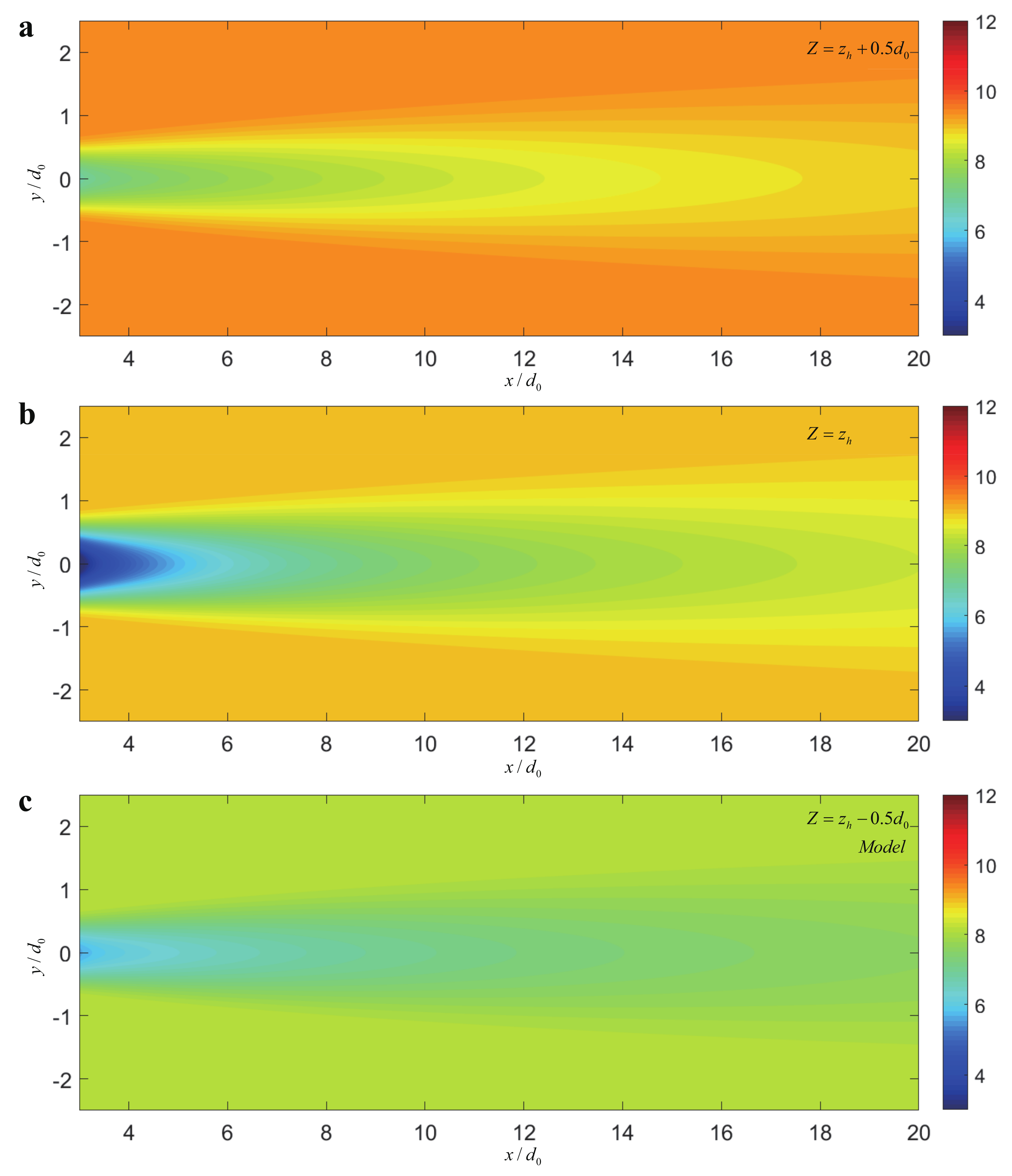
The Y – Z views of the streamwise velocity at different positions estimated by the model and LES are shown in Figure 15, among which the dashed line indicates rotor-sweeping region. The result shows that a slower recovery rate is noticed in the model compared with LES; this discrepancy becomes minor in further downwind distance (). Velocity distribution in Y – Z view obtained by the model was still in appropriate agreement with LES, and its non-axisymmetric characteristics were found because of the presence of the boundary layer. The figure shows that the wake circle is still clearly visible around and it gradually deforms due to the collision with the ground.
When the wind flows through a wind turbine, the torque exerted by the wind makes the turbine blades rotate. Due to the conservation of angular momentum, the wake rotates in the opposite direction to that of the blades. Given the theoretical difficulty in analytical models, there is no appropriate way to deal with the rotation effect. However, experimental [7] and numerical [49] studies found out flow rotation is not noticeable in the far wake (). Hence, the model is still competent to predict the streamwise velocity in the far wake region without consideration of the rotation effect.
5. Conclusions and Further Work
In this paper, a new analytical model is proposed to predict the velocity deficit in the wake downwind of a wind turbine. A cosine-shaped distribution is considered for the velocity deficit and mass and momentum conservation are employed to derive the model, which are expressed as:
where and are obtained by Equations (3) and (27) respectively. The effects of the ambient turbulence and the rotor generated turbulence are considered in the variable rate for wake expansion. Compared to the Tian model, which only employs mass conservation, this model makes use of the superiority of momentum conservation, filling a research gap in the development of cosine-series models.
The proposed model is tested against field observations, wind-tunnel measurements and high-resolution LES data, and the result shows that it can predict the velocity deficit downwind of a wind turbine with acceptable accuracy in terms of both shape and magnitude. By contrast, the top-hat models generally underestimate the velocity deficit at the wake center and overestimate it in proximity to the wake edge. Based on the new model, a series of predictions from different views are presented to demonstrate the wake-influenced region. The result indicates that wake effect is inconspicuous in the very far wake region and provides some references for the selection of wind turbines’ spacing. It should be noted that a major drawback of the model is that the analytical solution (Equation (23)) will diverge in the near wake region (–3), which prevents the model’s estimation of wake deficit near the rotor. However, due to its low computational cost, strong physics-based principles and good accuracy, this new model is still quite appealing for use in wind energy programs.
Future research will extend the capability of the proposed model to estimate the velocity deficit for different atmospheric stabilities. In addition, the model will be used to evaluate the power outputs of large wind farms for different layout configurations and inflow conditions.
Author Contributions
Conceptualization, Z.Z.; Formal analysis, Z.Z.; Investigation, Z.Z. and H.S.; Methodology, Z.Z.; Resources, P.H.; Supervision, P.H.; Writing—original draft, Z.Z. All authors have read and agreed to the published version of the manuscript.
Funding
This study was supported by Chinese National Natural Science Foundation (51678452), which is gratefully acknowledged.
Conflicts of Interest
The authors declare no conflict of interest.
References
- Perveen, R.; Kishor, N.; Mohanty, S.R. Off-shore wind farm development: Present status and challenges. Renew. Sustain. Energy Rev. 2014, 29, 780–792. [Google Scholar] [CrossRef]
- Vermeer, L.J.; Sorensen, J.N.; Crespo, A. Wind turbine wake aerodynamics. Prog. Aerosp. Sci. 2003, 39, 467–510. [Google Scholar] [CrossRef]
- Barthelmie, R.J.; Hansen, K.; Frandsen, S.T.; Rathmann, O.; Schepers, J.G.; Schlez, W.; Phillips, J.; Rados, K.; Zervos, A.; Politis, E.S.; et al. Modelling and Measuring Flow and Wind Turbine Wakes in Large Wind Farms Offshore. Wind Energy 2009, 12, 431–444. [Google Scholar] [CrossRef]
- Ishihara, T.; Qian, G.W. A new Gaussian-based analytical wake model for wind turbines considering ambient turbulence intensities and thrust coefficient effects. J. Wind Eng. Ind. Aerodyn. 2018, 177, 275–292. [Google Scholar] [CrossRef]
- Porté-Agel, F.; Bastankhah, M.; Shamsoddin, S. Wind-Turbine and Wind-Farm Flows: A Review. Bound. Layer Meteorol. 2019, 174, 1–59. [Google Scholar] [CrossRef] [PubMed] [Green Version]
- Barthelmie, R.J.; Pryor, S. An overview of data for wake model evaluation in the Virtual Wakes Laboratory. Appl. Energy 2013, 104, 834–844. [Google Scholar] [CrossRef]
- Zhang, W.; Markfort, C.D.; Porté-Agel, F. Near-wake flow structure downwind of a wind turbine in a turbulent boundary layer. Exp. Fluids 2012, 52, 1219–1235. [Google Scholar] [CrossRef] [Green Version]
- Howland, M.F.; Bossuyt, J.; Martineztossas, L.A.; Meyers, J.; Meneveau, C. Wake structure in actuator disk models of wind turbines in yaw under uniform inflow conditions. J. Renew. Sustain. Energy 2016, 8, 043301. [Google Scholar] [CrossRef] [Green Version]
- Bastankhah, M.; Porté-Agel, F. Wind tunnel study of the wind turbine interaction with a boundary-layer flow: Upwind region, turbine performance, and wake region. Phys. Fluids 2017, 29, 065105. [Google Scholar] [CrossRef]
- Abkar, M.; Sharifi, A.; Porteagel, F. Wake flow in a wind farm during a diurnal cycle. J. Turbul. 2016, 17, 420–441. [Google Scholar] [CrossRef]
- Qian, G.; Ishihara, T. A New Analytical Wake Model for Yawed Wind Turbines. Energies 2018, 11, 665. [Google Scholar] [CrossRef] [Green Version]
- Crespo, A. Survey of Modelling Methods for Wind Turbine Wakes and Wind Farms. Wind Energy 1999, 2, 1–24. [Google Scholar] [CrossRef]
- Gocmen, T.; Der Laan, P.V.; Rethore, P.; Diaz, A.P.; Larsen, G.C.; Ott, S. Wind turbine wake models developed at the technical university of Denmark: A review. Renew. Sustain. Energy Rev. 2016, 60, 752–769. [Google Scholar] [CrossRef] [Green Version]
- Jensen, N.O. A Note on Wind Generator Interaction; Risø National Laboratory: Roskilde, Denmark, 1983. [Google Scholar]
- Larsen, G.C. A Simple Wake Calculation Procedure; Risø National Laboratory: Roskilde, Denmark, 1988. [Google Scholar]
- Ishihara, T.; Yamaguchi, A.; Fujino, Y. Development of a new wake model based on a wind tunnel experiment. Glob. Wind Power 2004, 105, 33–45. [Google Scholar]
- Bastankhah, M.; Porté-Agel, F. A New Analytical Model For Wind-Turbine Wakes. Renew. Energy 2014, 70, 116–123. [Google Scholar] [CrossRef]
- Tian, L.; Zhu, W.; Shen, W.; Zhao, N.; Shen, Z. Development and validation of a new two-dimensional wake model for wind turbine wakes. J. Wind Eng. Ind. Aerodyn. 2015, 137, 90–99. [Google Scholar] [CrossRef] [Green Version]
- Gao, X.; Yang, H.; Lu, L. Optimization of wind turbine layout position in a wind farm using a newly-developed two-dimensional wake model. Appl. Energy 2016, 174, 192–200. [Google Scholar] [CrossRef]
- Sun, H.; Yang, H. Study on an innovative three-dimensional wind turbine wake model. Appl. Energy 2018, 226, 483–493. [Google Scholar] [CrossRef]
- Sun, H.; Yang, H. Study on three wake models’ effect on wind energy estimation in Hong Kong. Energy Procedia 2018, 145, 271–276. [Google Scholar] [CrossRef]
- Shao, Z.; Wu, Y.; Li, L.; Han, S.; Liu, Y. Multiple Wind Turbine Wakes Modeling Considering the Faster Wake Recovery in Overlapped Wakes. Energies 2019, 12, 680. [Google Scholar] [CrossRef] [Green Version]
- Barthelmie, R.J.; Folkerts, L.; Larsen, G.C.; Rados, K.; Pryor, S.C.; Frandsen, S.T.; Lange, B.; Schepers, G. Comparison of wake model simulations with offshore wind turbine wake profiles measured by sodar. J. Atmos. Ocean. Technol. 2006, 23, 888–901. [Google Scholar] [CrossRef]
- Frandsen, S. On the Wind-Speed Reduction in the Center of Large Clusters of Wind Turbines. J. Wind Eng. Ind. Aerodyn. 1992, 39, 251–265. [Google Scholar] [CrossRef]
- Hassan, G. GH WindFarmer: Theory Manual; Garrad Hassan and Partners Limited: Bristol, UK, 2003. [Google Scholar]
- Thørgersen, M.; Sørensen, T.; Nielsen, P.; Grötzner, A.; Chun, S. WindPRO/PARK: Introduction to wind turbine wake modelling and wake generated turbulence. In EMD Modelling and Wake Generated Turbulence; EMD International A/S: Aalborg, Denmark, 2005. [Google Scholar]
- Frandsen, S.; Barthelmie, R.; Pryor, S.; Rathmann, O.; Larsen, S.; Højstrup, J.; Thøgersen, M. Analytical modelling of wind speed deficit in large offshore wind farms. Wind Energy Int. J. Prog. Appl. Wind Power Convers. Technol. 2006, 9, 39–53. [Google Scholar] [CrossRef]
- Ge, M.; Wu, Y.; Liu, Y.; Yang, X. A two-dimensional Jensen model with a Gaussian-shaped velocity deficit. Renew. Energy 2019, 141, 46–56. [Google Scholar] [CrossRef]
- Chamorro, L.P.; Porté-Agel, F. A Wind-Tunnel Investigation of Wind-Turbine Wakes: Boundary-Layer Turbulence Effects. Bound. Layer Meteorol. 2009, 132, 129–149. [Google Scholar] [CrossRef] [Green Version]
- Wu, Y.T.; Porté-Agel, F. Atmospheric turbulence effects on wind-turbine wakes: An LES study. Energies 2012, 5, 5340–5362. [Google Scholar] [CrossRef]
- Xie, S.; Archer, C.L. A Numerical Study of Wind-Turbine Wakes for Three Atmospheric Stability Conditions. Bound. Layer Meteorol. 2017, 165, 87–112. [Google Scholar] [CrossRef]
- Stevens, R.J.A.M.; Meneveau, C. Flow Structure and Turbulence in Wind Farms. Annu. Rev. Fluid Mech. 2017, 49, 311–339. [Google Scholar] [CrossRef]
- Tian, L.; Zhu, W.J.; Shen, W.Z.; Song, Y.; Zhao, N. Prediction of multi-wake problems using an improved Jensen wake model. Renew. Energy 2017, 102, 457–469. [Google Scholar] [CrossRef]
- Niayifar, A.; Porte-Agel, F. Analytical Modeling of Wind Farms: A New Approach for Power Prediction. Energies 2016, 9, 741. [Google Scholar] [CrossRef] [Green Version]
- Xie, S.; Archer, C. Self-similarity and turbulence characteristics of wind turbine wakes via large-eddy simulation. Wind Energy 2015, 18, 1815–1838. [Google Scholar] [CrossRef]
- Abkar, M.; Porté-Agel, F. Influence of atmospheric stability on wind-turbine wakes: A large-eddy simulation study. Phys. Fluids 2015, 27, 035104. [Google Scholar] [CrossRef] [Green Version]
- Cheng, Y.; Zhang, M.; Zhang, Z.; Xu, J. A new analytical model for wind turbine wakes based on Monin-Obukhov similarity theory. Appl. Energy 2019, 239, 96–106. [Google Scholar] [CrossRef]
- Ge, M.; Wu, Y.; Liu, Y.; Li, Q. A two-dimensional model based on the expansion of physical wake boundary for wind-turbine wakes. Appl. Energy 2019, 233, 975–984. [Google Scholar] [CrossRef]
- Taylor, G. Wake Measurements on the Nibe Wind-Turbines in Denmark; National Power, Technology and Environment Centre: Leatherhead, UK, 1990. [Google Scholar]
- Schlez, W.; Tindal, A.; Quarton, D. GH Wind Farmer Validation Report; Garrad Hassan and Partners Ltd: Bristol, UK, 2003. [Google Scholar]
- Tennekes, H.; Lumley, J.L.; Lumley, J.L. A First Course in Turbulence; MIT Press: Cambridge, MA, USA, 1972. [Google Scholar]
- Burton, T.; Jenkins, N.; Sharpe, D.; Bossanyi, E. Wind Energy Handbook; John Wiley & Sons: Hoboken, NJ, USA, 2011. [Google Scholar]
- Sun, H.; Yang, H. Numerical investigation of the average wind speed of a single wind turbine and development of a novel three-dimensional multiple wind turbine wake model. Renew. Energy 2020, 147, 192–203. [Google Scholar] [CrossRef]
- Quarton, D.; Ainslie, J. Turbulence in wind turbine wakes. Wind Eng. 1990, 14, 15–23. [Google Scholar]
- Hassan, U. A Wind Tunnel Investigation of the Wake Structure within Small Wind Turbine Farms; Harwell Laboratory, Energy Technology Support Unit: Harwell, UK, 1993. [Google Scholar]
- Crespo, A.; Hernández, J. Turbulence characteristics in wind-turbine wakes. J. Wind Eng. Ind. Aerodyn. 1996, 61, 71–85. [Google Scholar] [CrossRef]
- Troldborg, N.; Sørensen, J.N.; Mikkelsen, R.; Sørensen, N.N. A simple atmospheric boundary layer model applied to large eddy simulations of wind turbine wakes. Wind Energy 2014, 17, 657–669. [Google Scholar] [CrossRef]
- Lissaman, P.B.S. Energy Effectiveness of Arbitrary Arrays of Wind Turbines. J. Energy 1979, 3, 323–328. [Google Scholar] [CrossRef]
- Porté-Agel, F.; Wu, Y.T.; Lu, H.; Conzemius, R.J. Large-eddy simulation of atmospheric boundary layer flow through wind turbines and wind farms. J. Wind Eng. Ind. Aerodyn. 2011, 99, 154–168. [Google Scholar] [CrossRef]
Figure 1.
Schematic of the linear wake expansion in the Jensen model.
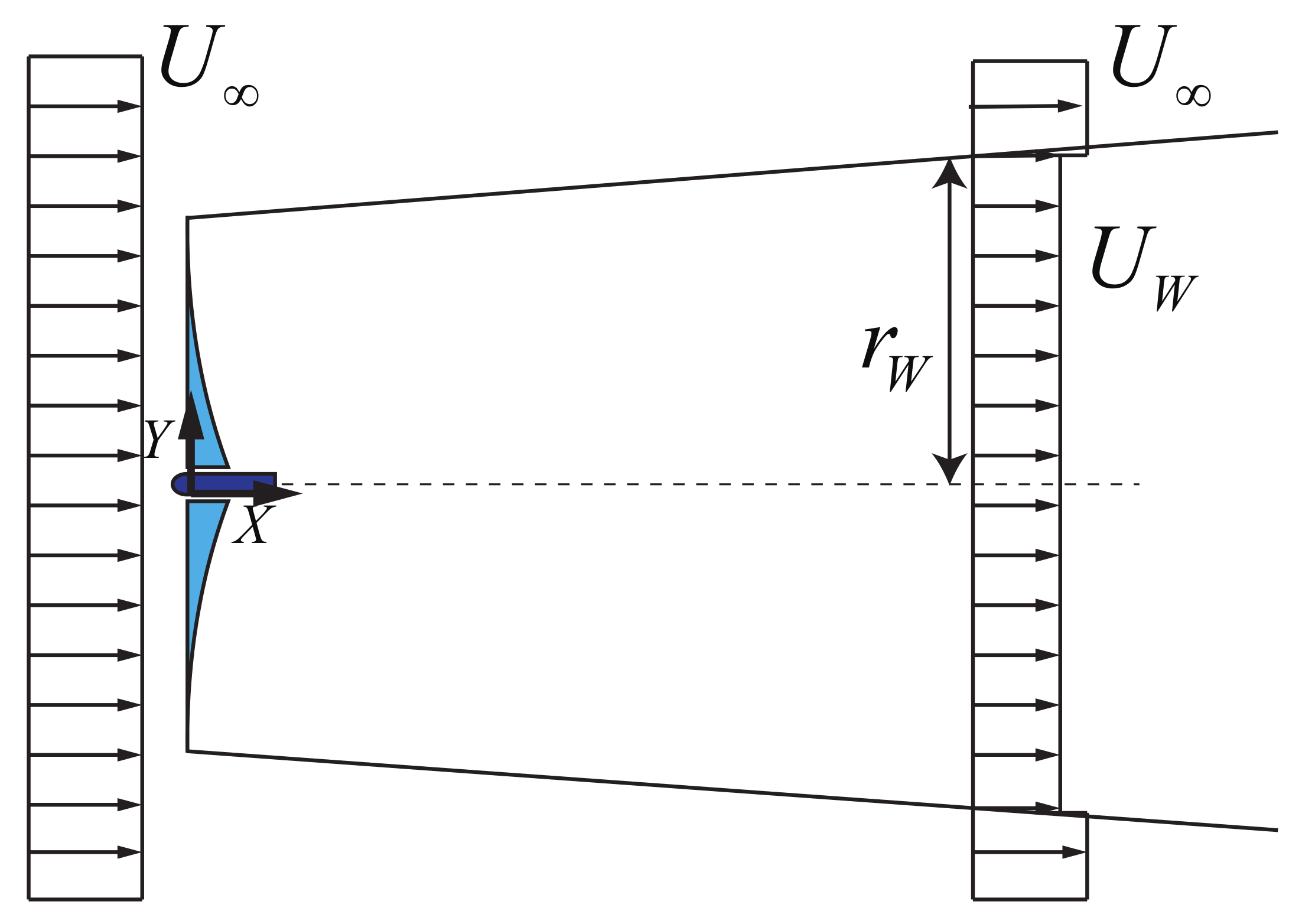
Figure 2.
Schematic of the control volume around the wind turbine.
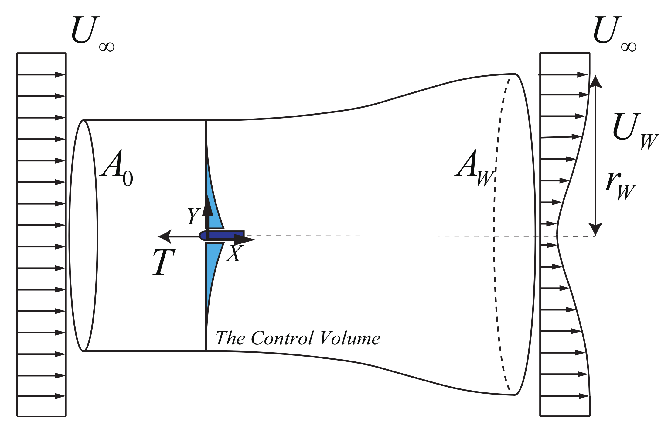
Figure 3.
Assumption of the trigonometric distribution for velocity deficit.
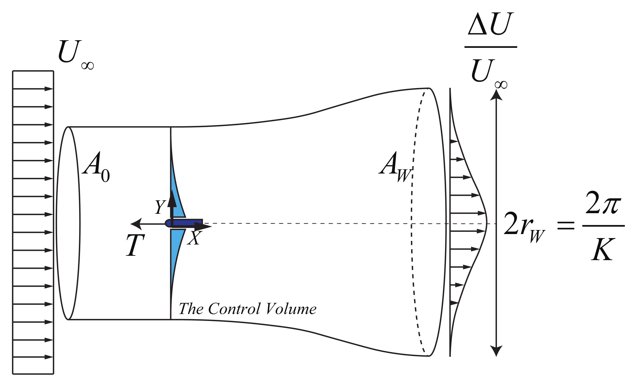
Figure 4.
Turbulence intensity at the top tip height estimated by the Crespo and Hernández model and the Ishihara and Qian model.
Figure 4.
Turbulence intensity at the top tip height estimated by the Crespo and Hernández model and the Ishihara and Qian model.
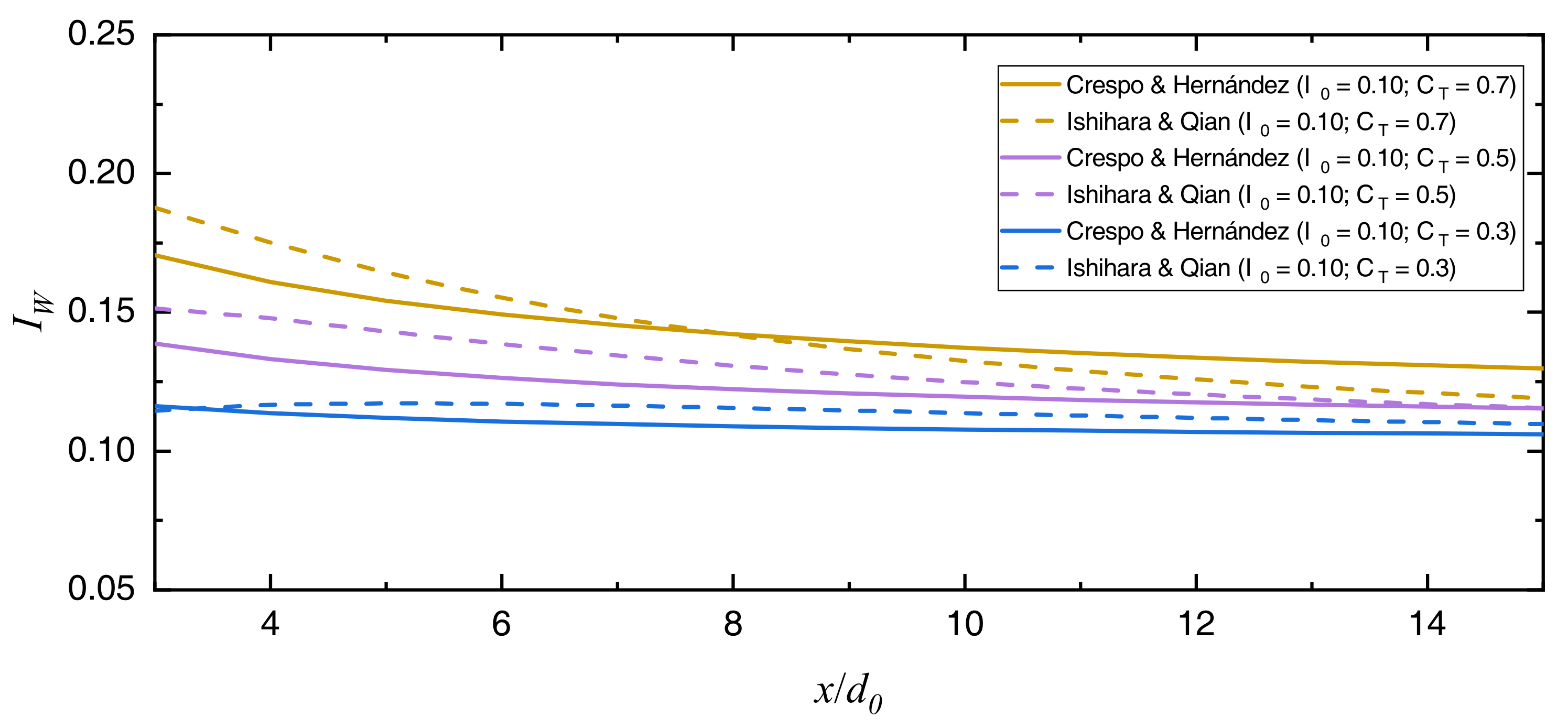
Figure 5.
A flowchart of development and validation of the proposed model.
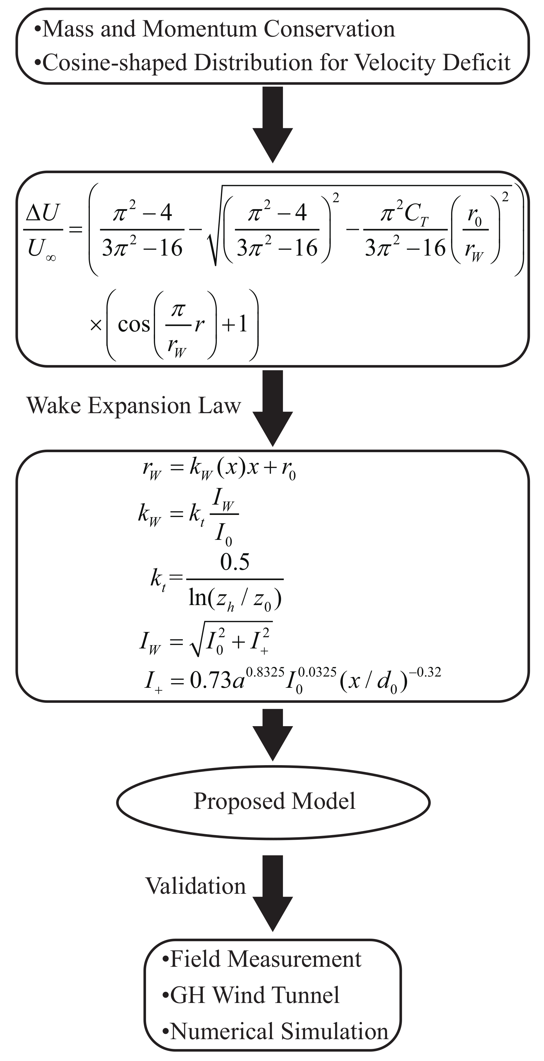
Figure 6.
Sketch of the Nibe site.
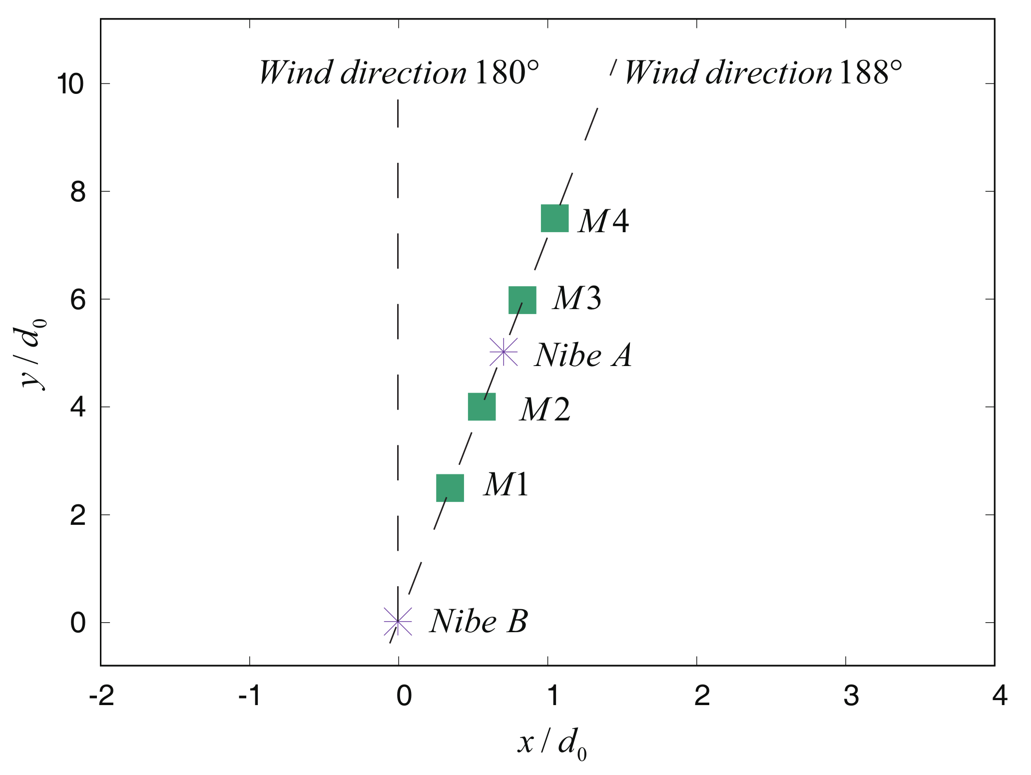
Figure 7.
Comparison between the field measurement data and the predicted normalized velocity deficit: (a) ; (b) .
Figure 7.
Comparison between the field measurement data and the predicted normalized velocity deficit: (a) ; (b) .
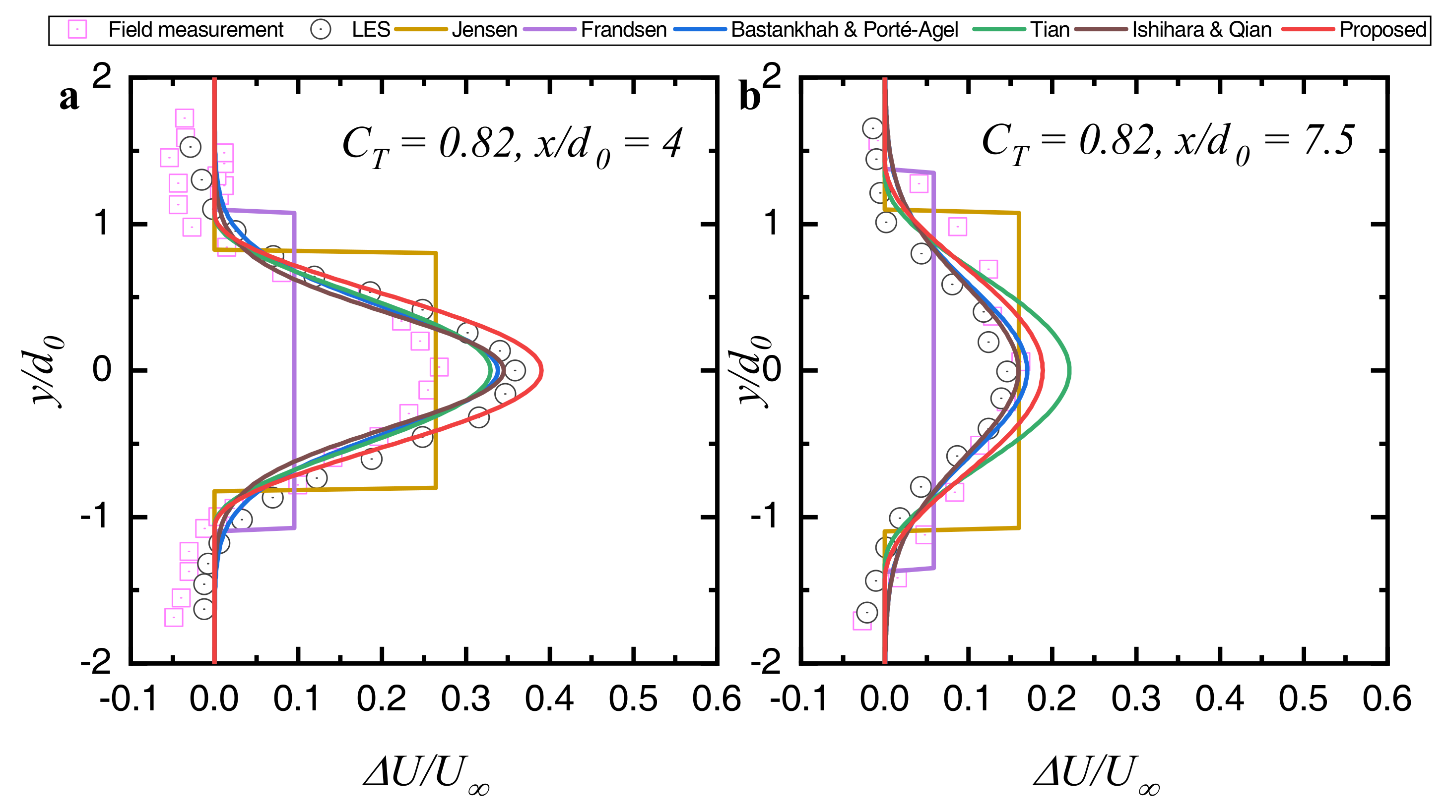
Figure 8.
Comparison between the wind-tunnel measurement data and the predicted normalized velocity deficit: (a) ; (b) ; (c) ; (d) .
Figure 8.
Comparison between the wind-tunnel measurement data and the predicted normalized velocity deficit: (a) ; (b) ; (c) ; (d) .
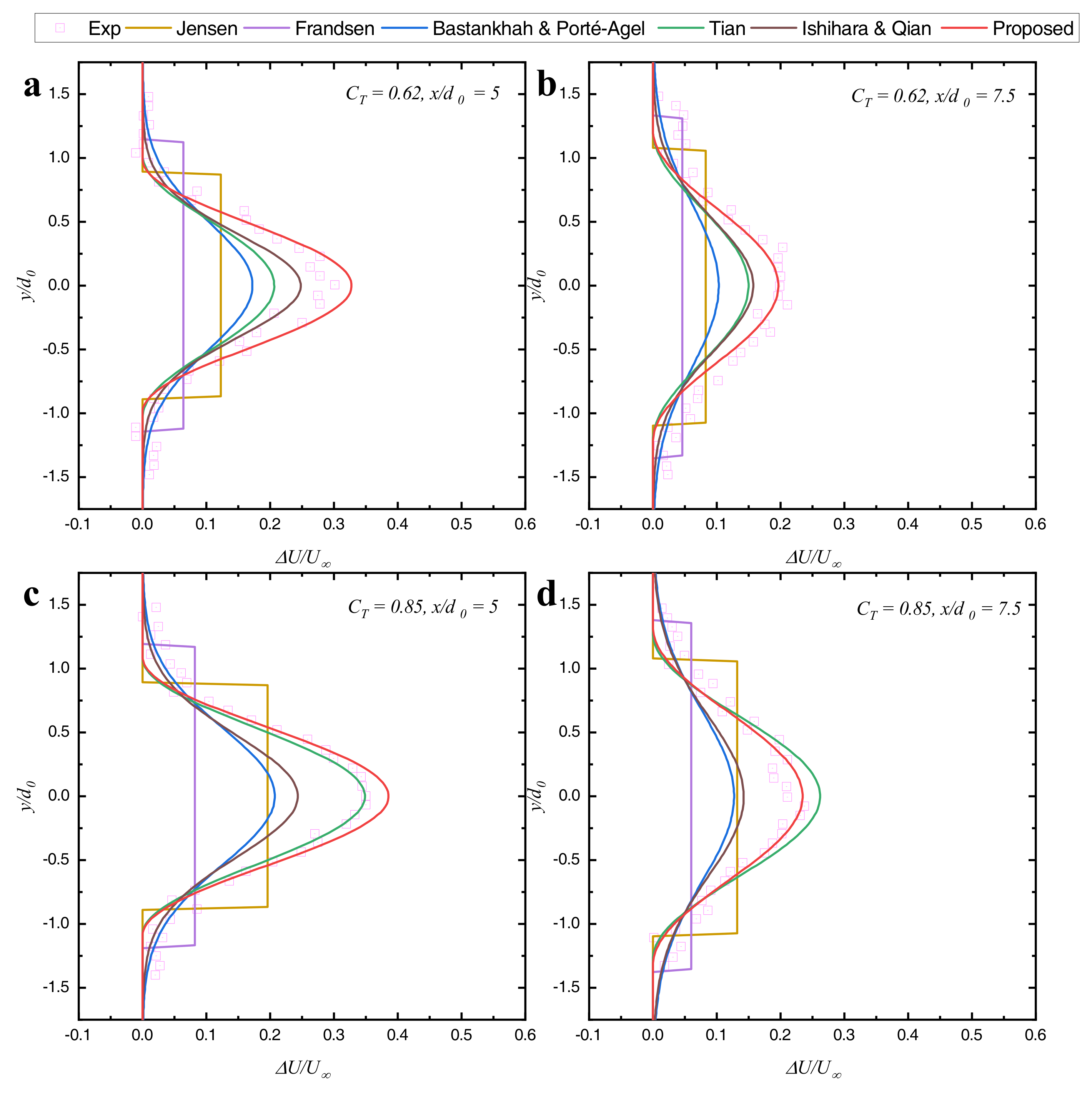
Figure 9.
Comparison between the numerical simulation data and the predicted normalized velocity deficit in horizontal (top) and vertical (bottom) profiles: (a) m, (horizontal); (b) m, (horizontal); (c) m, (vertical); (d) m, (vertical); (e) m, (horizontal); (f) m, (horizontal); (g) m, (vertical); (h) m, (vertical).
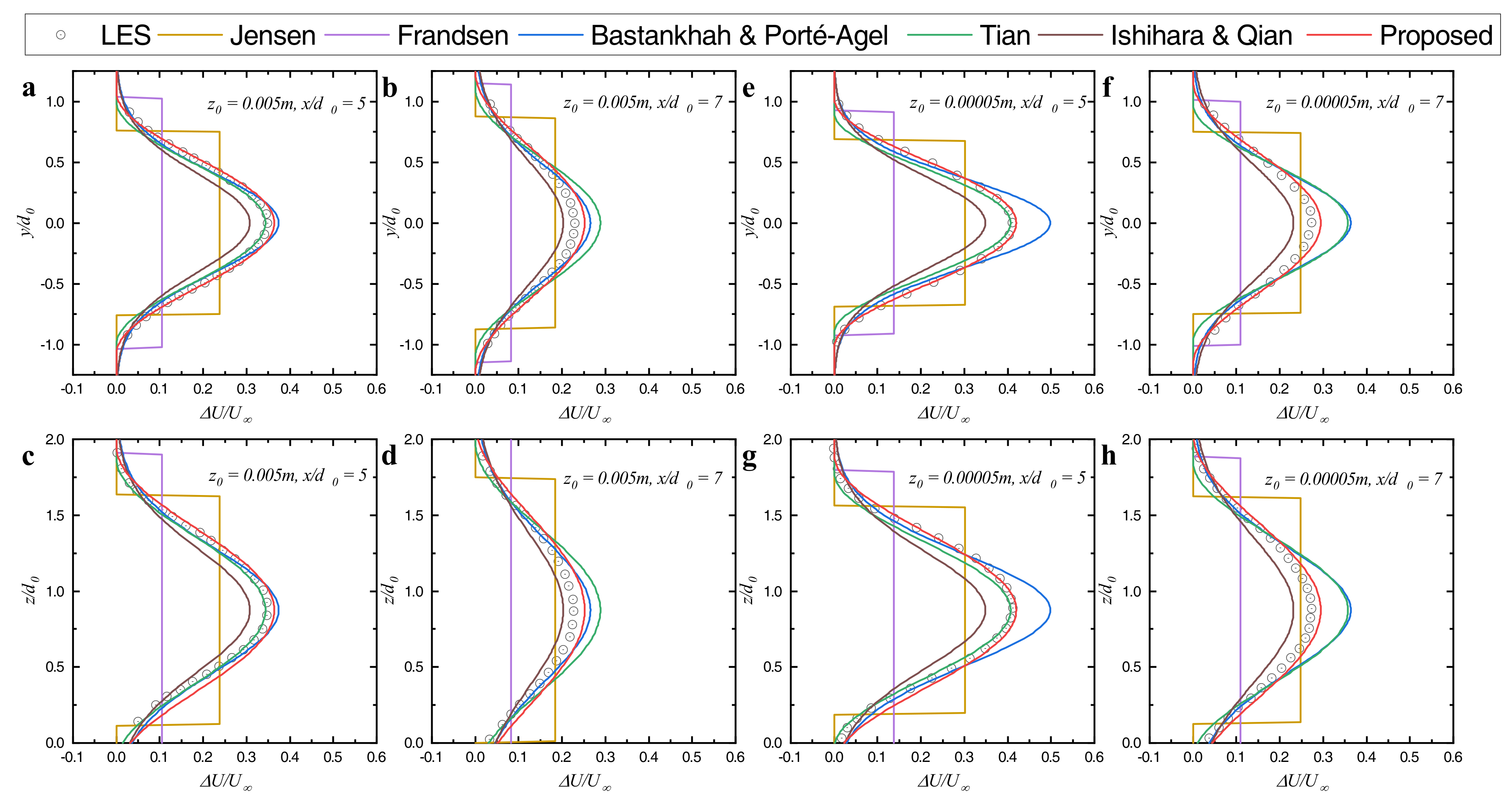
Figure 10.
Comparison between the numerical simulation data and the predicted maximum normalized velocity deficit downwind of the wind turbine: (a) m; (b) m.
Figure 10.
Comparison between the numerical simulation data and the predicted maximum normalized velocity deficit downwind of the wind turbine: (a) m; (b) m.
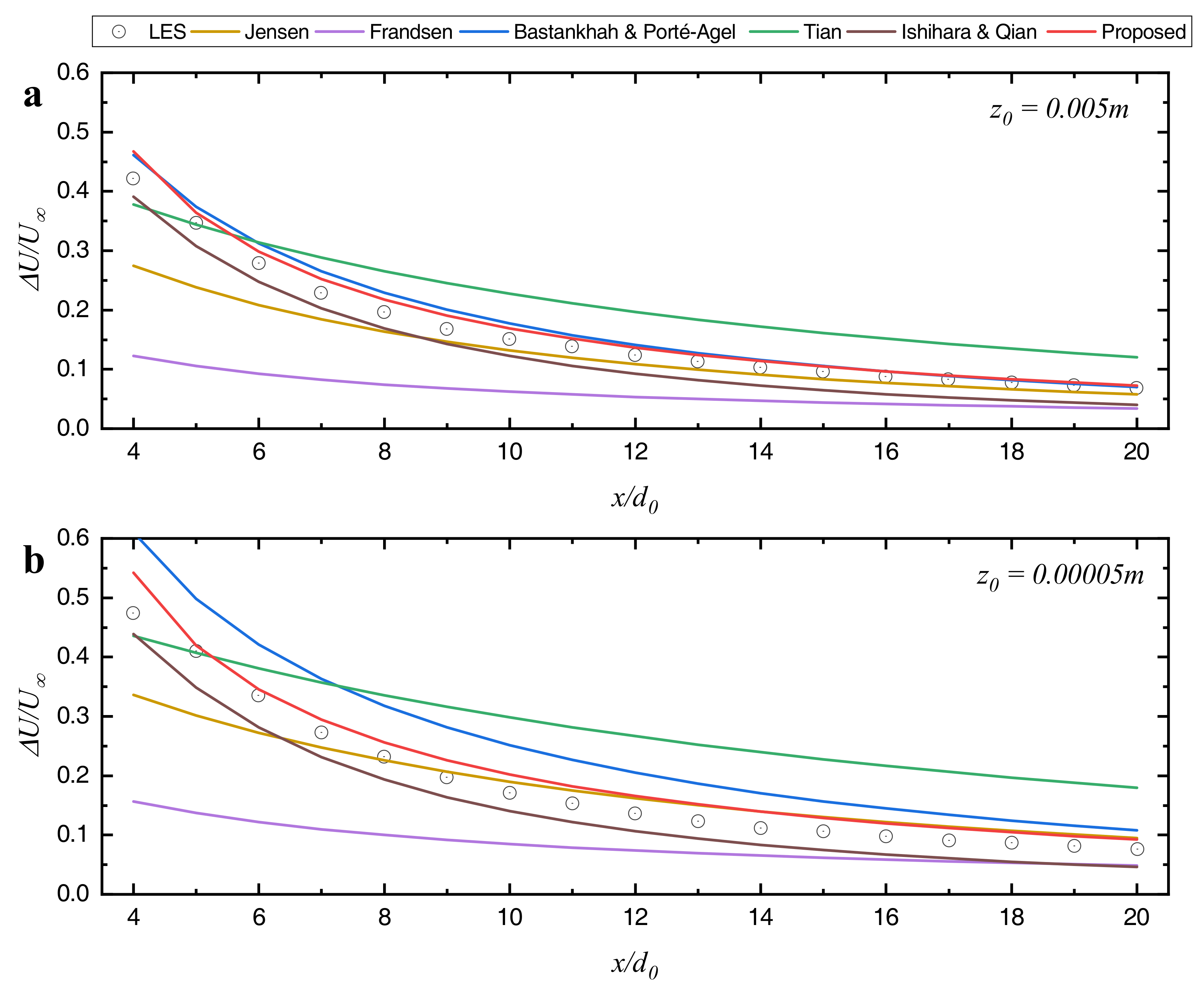
Figure 11.
Schematic of the vertical profile of (a) streamwise velocity and (b) velocity deficit.
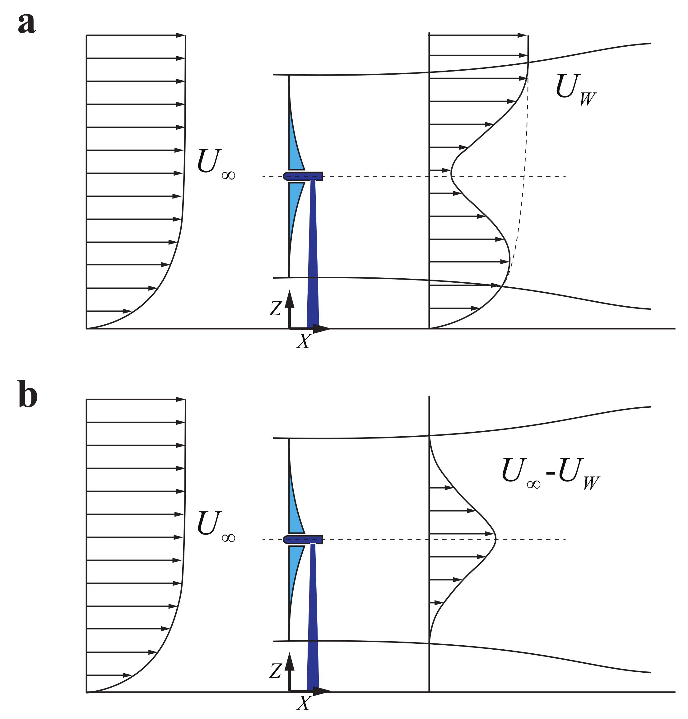
Figure 12.
X – Y views of the streamwise velocity estimated by the model: (a) ; (b) ; (c) .

Figure 13.
X – Z views of the streamwise velocity at estimated by (a) the model and (b) LES (reproduced with permission from Wu and Porté-Agel [30]).
Figure 13.
X – Z views of the streamwise velocity at estimated by (a) the model and (b) LES (reproduced with permission from Wu and Porté-Agel [30]).
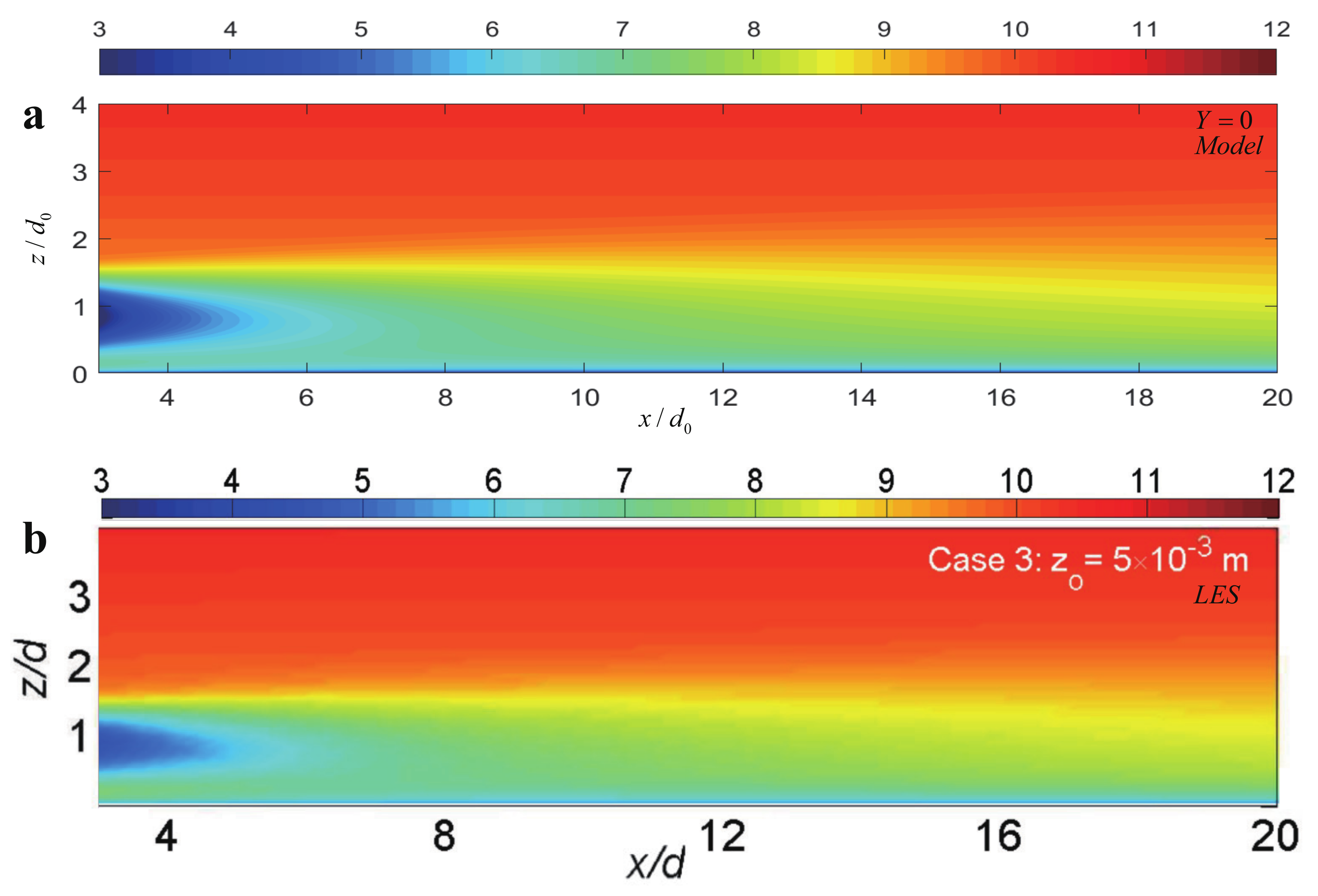
Figure 14.
X – Z views of the streamwise velocity estimated by the model: (a) ; (b) ; (c) ; (d) ; (e) .
Figure 14.
X – Z views of the streamwise velocity estimated by the model: (a) ; (b) ; (c) ; (d) ; (e) .
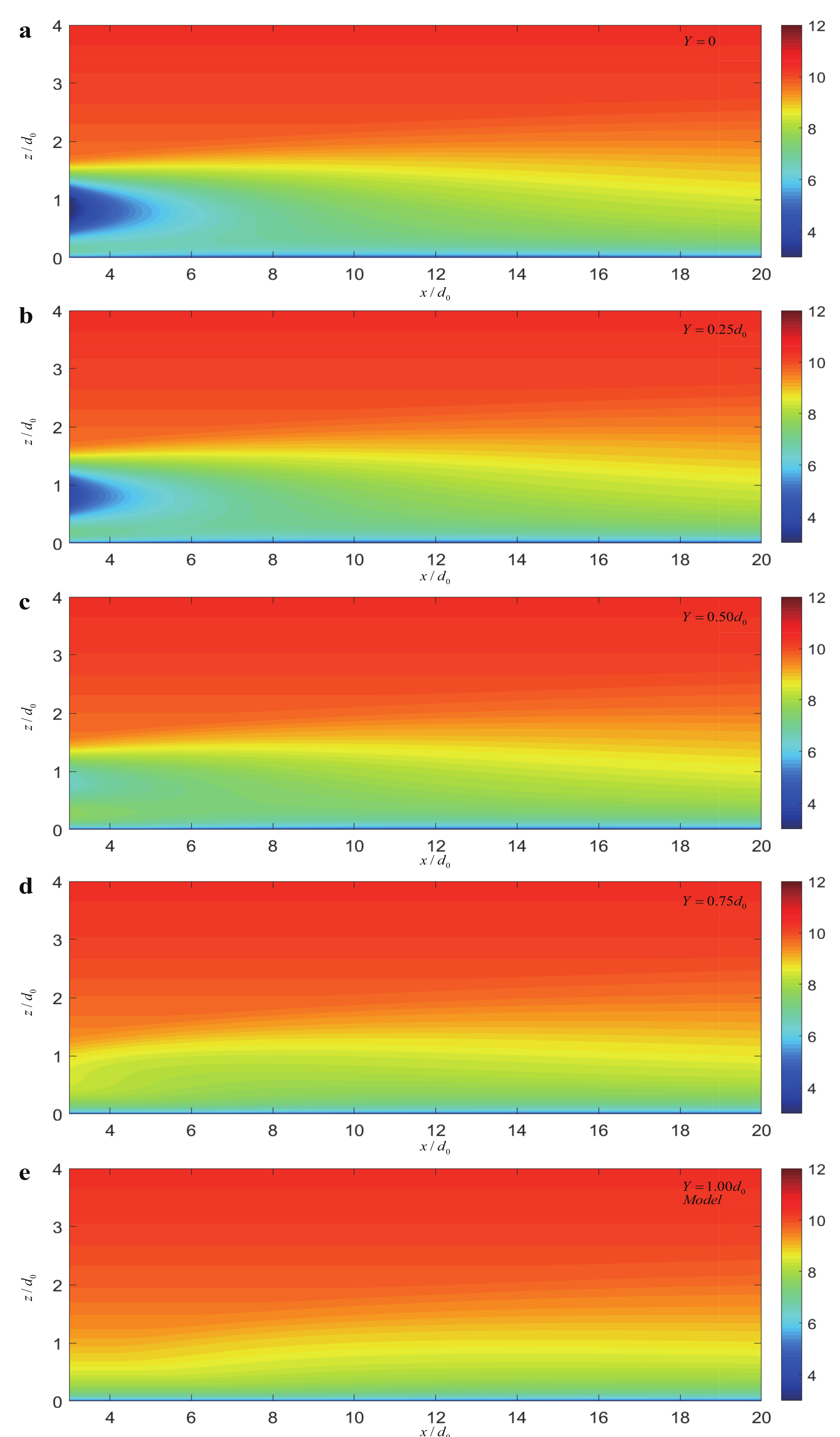
Figure 15.
Y – Z views of the streamwise velocity estimated by (a) the model and (b) LES (reproduced with permission from Wu and Porté-Agel [30]).
Figure 15.
Y – Z views of the streamwise velocity estimated by (a) the model and (b) LES (reproduced with permission from Wu and Porté-Agel [30]).


Table 1.
Comparison between the proposed model and the previous wake models.
| Characteristics | Jensen | Frandsen | Bastankhah & Porté-Agel | Tian | Proposed |
|---|---|---|---|---|---|
| Profile | Top-hat | Top-hat | Gaussian | Cosine | Cosine |
| Principles | MC | MC&MT | MC&MT | MC | MC&MT |
| Wake expansion law | Linear | Nonlinear | Linear | Nonlinear | Nonlinear |
| Expansion coefficient |
MC: mass conservation; MT: momentum theory.
Table 2.
Relative errors of the models in two cases with different roughness lengths.
| Relative Error (%) | Jensen | Frandsen | Bastankhah & Porté-Agel | Tian | Ishihara & Qian | Proposed |
|---|---|---|---|---|---|---|
| m | 17.1 | 58.2 | 11.0 | 50.3 | 24.8 | 9.0 |
| m | 18.9 | 49.1 | 41.4 | 81.1 | 24.1 | 16.7 |
© 2020 by the authors. Licensee MDPI, Basel, Switzerland. This article is an open access article distributed under the terms and conditions of the Creative Commons Attribution (CC BY) license (http://creativecommons.org/licenses/by/4.0/).
Share and Cite
MDPI and ACS Style
Zhang, Z.; Huang, P.; Sun, H. A Novel Analytical Wake Model with a Cosine-Shaped Velocity Deficit. Energies 2020, 13, 3353. https://doi.org/10.3390/en13133353
AMA Style
Zhang Z, Huang P, Sun H. A Novel Analytical Wake Model with a Cosine-Shaped Velocity Deficit. Energies. 2020; 13(13):3353. https://doi.org/10.3390/en13133353
Chicago/Turabian StyleZhang, Ziyu, Peng Huang, and Haocheng Sun. 2020. "A Novel Analytical Wake Model with a Cosine-Shaped Velocity Deficit" Energies 13, no. 13: 3353. https://doi.org/10.3390/en13133353
Note that from the first issue of 2016, this journal uses article numbers instead of page numbers. See further details here.