A CFD Investigation of a 2D Balanced Vane Pump Focusing on Leakage Flows and Multiphase Flow Characteristics

Abstract

Vane pumps are often applied in automatic transmission systems of vehicles. Future applications require the oil pumps to be more efficient and to be able to handle multiphase flow pumping situations to a certain extend. To fulfill these requirements, efficient development tools are needed. Therefore, a less demanding computational 2D model of a fixed-type balanced vane pump was derived and numerically analyzed with the commercial computational fluid dynamics (CFD) software ANSYS CFX. The meshing of the rotating parts was done with TwinMesh, using a moving mesh approach. At first, a mesh convergence study was performed. It was shown that the resolution of the radial clearances in particular had a significant influence on the predicted leakages and the volumetric efficiency. The leakage was further investigated concerning the dependence on rotational speed and delivery pressure. In the next step, multiphase flows were considered. In a first setup, vapor cavitation was analyzed and the influence of the alignment of the suction ports on its onset was derived. In a second setup, the influence of different inlet volume fractions of free air was evaluated. The employed multiphase modeling approach was presented and a sensitivity analysis on modeling parameters was performed. Overall, it was shown that free air in the suction ports changed the pumping characteristic of the vane pump significantly. Pressure and flow ripple increased, and the volumetric efficiency and the mean power demand decreased significantly with an increasing inlet volume fraction.

1. Introduction

Vane pumps represent an important type of positive displacement pumps, which are applied in many different hydraulic systems [1]. In the last years, this pump type is also more and more commonly applied in automatic transmission oil circuits for passenger cars, as well as for commercial vehicles [2]. Despite its weak quick start ability and a high susceptibility regarding dirt particles, its high specific performance, good efficiency, adaptability, and variability, as well as its acoustic characteristics, make it a suitable fit for the requirements of these systems [1,3,4,5,6]. The applied pump acts as a hydraulic supply to deliver the required oil flow rate for the transmission system components to be lubricated and cooled, and the required hydraulic pressure to actuate internal clutches and brakes.

The working principle of a vane pump is as follows: A rotor with radial slots is placed inside a cam ring. A certain number of vanes can radially slide in and out of the rotor and when moving along the cam ring, they form displacement chambers. Centrifugal forces ensure that the vanes slide along the cam ring and seal the different chambers from each other. The eccentricity of the rotor with respect to the cam ring leads to a periodic change of chamber volume within one rotor revolution. In the region where the chamber volume increases, the fluid is pulled into the displacement chambers radially or axially through a suction port. When the chamber volume decreases again, grooves connect the chamber to the delivery port and the fluid is conveyed. In between, the displacement chamber is sealed, except for the inherent radial and axial gaps, which are responsible for the internal volumetric losses. In positive displacement pumps, these clearances are typically a few micrometers in height [1].

Vane pumps can be designed to be of a double stroke type, as displayed in Figure 1. Within one rotor revolution, two suction and two pressure ports are served. This means the pump can supply two different hydraulic circuits with different pressures loads and volumetric flow rates at once. If both operate with the same displacement volume and at the same pressure load, the acting forces are symmetrically distributed and the pump is called a balanced vane pump. This adaptability to serve two different hydraulic circuits is an important advantage of vane pumps [1].

Currently, the automatic transmission market changes rapidly. The market shares of different transmission types are shifting worldwide. Furthermore, electrified powertrains are gaining an everyday growing market share. This leads to changing requirements for the respective hydraulic supplies. These accessories influence the fuel consumption or the range of electric vehicles significantly. Therefore, a higher overall efficiency and, consequently, a higher volumetric efficiency of the pumps become more and more important. Furthermore, in modern transmission systems, there are often situations in which the pump has to handle multiphase flow as foam or even bigger air bubbles are conveyed into the oil circuit. However, the pump has to fulfill the hydraulic requirements of the system. Cavitation as another multiphase flow phenomenon also limits the operational range of the hydraulic pump and should therefore be avoided. The acoustic characteristic of the pumps is crucial as well, since the powertrains become more silent these days and therefore do not mask the noise of the pumps anymore.

Due to these requirements, a better insight into the internal leakages, as well as the multiphase pumping characteristic of balanced vane pumps are needed to develop suitable pumps for future transmission applications.

To investigate and optimize vane pumps, experimental methods are important. In the work of [7], the authors experimentally investigate ways to improve the volumetric and mechanical efficiency of a small vane pump, which is also applied in automatic transmission systems.

Additionally, there are different approaches to theoretically model and analyze vane pumps. On the one hand, 0D- and 1D-lumped parameter models have to be mentioned. In [8], the authors analyze and optimize the vane-cam ring kinematics in a balanced vane pump analytically. The same authors include analytical functions to calculate the resulting theoretical flow rates within their model in their publication of 2020 [9]. Balanced vane pumps are investigated regarding their suitability of operating with water by experimental and analytical means by Lu et al. in [10]. The authors employ an analytical leakage model to predict the volumetric efficiency of the pumps. In [11], the authors investigate a vane pump with the commercial system simulation software AMESim. They mostly use analytical equations to model the leakages and the conveying characteristic. Another comprehensive analysis of a variable displacement vane pump with a hydraulic model developed by the authors is presented in [12]. The work focuses on flow and pressure ripple, and incorporates cavitation phenomena. In [13], the authors present a 1D model of a vane pump with the commercial hydraulic system simulation software GT-SUITE, which incorporates frictional losses as well as leakages.

On the other hand, there is the possibility to employ a full 3D computational fluid dynamics (CFD) simulation to incorporate all fluid dynamic effects that can be observed in a real pump. Therefore, an appropriate method to mesh the deforming and moving displacement chambers of the pump has to be applied. In [14], the authors present a model with the CFD software PumpLinx. PumpLinx was specifically developed for the 3D simulation of positive displacement pumps. The work focuses on cavitation and validation of the numerical results with experimental data. PumpLinx is also used in [15] to investigate the influence of an asymmetrical cam ring curve for a sliding vane vacuum pump numerically. In addition, in [16], another CFD study with PumpLinx of a balanced vane pump is presented.

In [17], the authors present a multiphase study in ANSYS Fluent for a vacuum vane pump incorporating air and lubricating oil with a volume of fluid method. They use a redefinition algorithm for the mesh deformation and movement. Another method for grid and boundary generation, as well as discretization of a vacuum vane pump for ANSYS CFX and Fluent, is presented in [18].

A study on cavitation in a reciprocating positive displacement pump has been performed with ANSYS Fluent in [19], where non-condensable air was also incorporated by applying the full cavitation model. The effects of entrained air, however, are only partly analyzed with the applied full cavitation model. This model is limited as it uses a homogeneous approach; hence, phase separation and slip velocities between both phases are not incorporated. Furthermore, the used three-fluid approach is highly unstable at higher rotational speeds and very sensitive regarding mesh quality.

There are a lot of CFD studies of multiphase flows containing a continuous liquid phase and a dispersed bubbly air phase for centrifugal pumps. One example is [20], where a bubbly flow is analyzed with ANSYS CFX. Yet, these do not incorporate clearances as tight as they are present in the fluid domain of positive displacement pumps. There is clearly a gap of such multiphase studies for positive displacement pumps [21].

One reason may be the high requirements of the numerical schemes regarding the mesh quality. Cell aspect ratios need to be small and minimum angles also need to be quite high compared to single-phase simulations. This is especially difficult to achieve in the tight clearances of positive displacement pumps. Additionally, those tight clearances are the locations, where the highest-pressure gradients and therefore velocities occur. Because of that, the required total cell count for a 3D case is very high. To reduce the computational effort and therefore to be able to investigate the influence of more parameters, it was decided to use a simplified 2D model, which is derived from a reference pump. The aim of this paper is to gain the understanding of the conveying characteristics of the 2D balanced vane pump. The leakages and their correct prediction, which govern the calculated volumetric efficiency, are a particular focus point. As there were only radial leakage gaps in the 2D case, these could be analyzed without the influence of axial gaps. The second focus point is to analyze the operating characteristics of the pump with free air inlet gas volume fractions (IGVF) present. Outlet pressure and flow rate ripple, displacement chamber pressure profiles, power demand, and, of course, volumetric efficiency were significantly influenced by introducing free air. Furthermore, the influences of the multiphase modeling approaches and their parameters are investigated.

2. CFD Model of the 2D Vane Pump

The 2D vane pump model, as it is shown in Figure 2, is derived from a Bosch fixed displacement balanced vane pump with twelve vanes of a thickness of 1.4 mm and a displacement volume of $V_{displ,3D}$ = 14.8 cm³/rev. This pump was applied in the oil circuit of torque converter automatic transmission systems. The pump’s rotor had a diameter of 39 and a height of 16 mm. The small cam ring diameter was 51 and the large cam ring diameter was 57 mm.

As the solver ANSYS CFX is not capable to solve 2D space domains, at least one computational cell layer in the third dimension is necessary. The height of the model in this direction was set to 30 µm. This value was used to obtain small cell aspect ratios < 100 and a good similitude of occurring Reynolds numbers in the 2D and the respective 3D case. This resulted in a displacement volume of $V_{displ,2D}$ = 0.028 cm³/rev.

In real vane pumps, radial gap heights of h = 2–10 µm between the vane tips and the cam ring can be assumed for most common operating points [1]. In this 2D model, the radial gap height was set to 50 µm. This enlarged value was due to numerical limitations. As there was no third dimension available for diffusion processes and the flow cross section in the radial gaps was very small, the occurring pressure gradients and velocities in the 2D case were much higher than in a 3D case. This led to numerical issues, especially when solving a multiphase flow field. Therefore, no convergence could be obtained with radial gap heights h < 50 µm.

At inlets 1 and 2, the pressure boundary conditions were set to 1 bar absolute pressure. At both outlets, the same delivery pressure was specified as another boundary condition. Because of that, the conveying of the fluid solely resulted from the mesh movement with a specified rotational speed.

The radial gaps presented the only leakage paths from the delivery to the suction port in this 2D case. In Figure 3, it is displayed that from each delivery port there are two possible leakage paths back to the two suction ports. The first path, defined as radial gap 1, with a leakage mass flow rate ${\dot{m}}_{leakage1}$, had a driving pressure gradient which was aligned against the direction of rotation of the pump rotor. The other leakage path, defined as radial gap 2 with ${\dot{m}}_{leakage2}$, had a driving pressure gradient which was aligned in the direction of rotor rotation. Axial gaps, which are in reality 5–15 µm in height and are located axially between the vanes and the housing of the pump, were missing in this 2D setup. Therefore, it could be assumed that the predicted volumetric efficiency of the 2D model, as it is defined in Equation (1), had to be higher than in a real 3D case. The enlarged radial gaps, however, compensated this effect to a certain extent and contributed to higher leakage flows. The theoretical volumetric flow rate $Q_{theo}$ of the pump was calculated by multiplying the displacement volume $V_{displ}$ with the rotational speed n:

$${\eta }_{vol}=\frac{Q_{actual}}{Q_{theo}}=\frac{Q_{theo}-Q_{leakage}}{Q_{theo}} with Q_{theo}=V_{displ}·n$$

(1)

For the meshing of the displacement chambers, which rotate and change in size and shape, a moving mesh approach was applied with the commercial software TwinMesh. Structured hexahedral meshes for a specified angular step size were generated in advance of the solver run [22]. The generated meshes had an O-shaped topology, as can be seen in Figure 2. Therefore, all radial cell layers were present in the displacement chamber as well as in the radial gaps. The maximum cell size was 0.5 mm.

The stator parts, namely the two suction ports and the two delivery ports, were both spatially discretized with an unstructured mesh with a base size of 3 mm. On the interface toward the rotating parts and on the walls, prism layers were applied, where the first cell layer ensured a value of y+ < 30 for the applied wall function of the turbulence model. For the modeling of the multiphase flow phenomena, two independent approaches were selected, which are both displayed in

Table 1. Overview of setups for multiphase flow simulations.

	Setup 1 (Cavitation)		Setup 2 (IGVF of Air)
Simulation method	RANS, unsteady		RANS, unsteady
Euler–Euler approach	homogeneous		inhomogeneous
Phases	Liquid oil	Oil vapor	Liquid oil	Air (ideal gas)
Phase morphology	Continuous	Continuous	Continuous	Dispersed
Turbulence model	k-ω SST		k-ω SST	Dispersed Phase Zero equation
Interphase transfer	-		Particle model, 0.1 mm mean bubble diameter
Mass transfer	Rayleigh–Plesset, 2 µm mean bubble diameter		-
Momentum transfer	-		Schiller–Naumann
Heat transfer	-		Ranz–Marshall
Turbulence transfer	-		SATO enhanced eddy viscosity
Buoyancy	-		Density difference

.

For both cases, an Euler–Euler approach was chosen. In this approach, both phases generally shared a common pressure field.

Setup 1 was able to capture the effects of vapor cavitation. Therefore, a homogeneous two-phase flow field of liquid oil and oil vapor was set up. Due to the assumption of a homogeneous flow field, both phases also shares a common velocity and temperature field. The used fluid properties of the oil are listed in

Table 2. Fluid properties of the automatic transmission oil at 20 °C and 1 bar.

Density (kg/m3)	843
Dyn. viscosity (Pa$·$s)	0.07485
Liquid bulk modulus (Pa)	$1.5·{10}^9$
Surface tension oil-air (N/m)	$2.5·{10}^{-2}$
Vapor pressure (Pa)	30
Specific heat capacity (J/(kg$·$K))	1781
Thermal conductivity (W/(m$·$K))	0.142

. Turbulence was also homogeneously modeled with the k-ω shear stress transport (SST) model being active in both phases. For the mass transfer between both phases, which incorporates vapor cavitation, the Rayleigh–Plesset cavitation model was chosen. Both phases were assumed to be continuous, which was a valid assumption when modeling cavitation with the Rayleigh–Plesset model [23]. Besides the mass transfer, no further interphase transfers were modeled. The mean diameter for the generated oil vapor bubbles was assumed to be 2 µm, which is a standard value in hydraulics. All other model constants were also set to the standard values. More information about these model constants and their validity can be found in [23].

Setup 2 was used to investigate the effects of a bubbly oil–air flow by introducing volume fraction boundary conditions for free air at the two inlets (IGVF). Therefore, an inhomogeneous two-phase flow of liquid oil and air, modeled as an ideal gas, was set up. The phases only shared a common pressure field. The oil phase was assumed to be continuous while the air phase was modeled as a dispersed phase with bubbles of a mean diameter of 0.1 mm. This assumption was based on experiments in transmission oil circuits. The influence of the inhomogeneous flow field approach, as well as of the mean diameter, are investigated later on in this paper. Buoyancy was also modeled with the gravitational acceleration vector being oriented in the negative y-direction. Turbulence was incorporated with the dispersed phase zero equation model in the air phase, while the SST model was applied in the oil phase. The surface tension of the air bubbles was also considered. For interphase transfer terms, the particle model was applied. It assumed a spherical interface area. While the drag was modeled by the Schiller–Naumann model, for the heat transfer, the Ranz–Marshall model was used. The SATO enhanced eddy viscosity model incorporated turbulence transfer between both phases. No mass transfer between the two phases was incorporated in setup 2.

3. Derivation of Analytical Solutions for the Circumferential Velocity Profile in the Radial Gap

To investigate the leakages through the radial gaps in detail, the developing circumferential velocity profiles were of special interest. Therefore, a simplified model for the radial gap was introduced, which is described in Figure 4. It was assumed that the radial gaps can be modeled by two concentric, cylindrical walls. The inner wall, which represents the vane tip, rotated with an angular velocity, while the outer wall, which represents the cam ring, was not moving, i.e., ${\omega }_2=0$ rad/s. Furthermore, a constant pressure gradient in the circumferential direction $\frac{\partial p}{\partial \phi }$ was assumed.

With these assumptions and under the premise of an incompressible and stationary two-dimensional flow, the Navier–Stokes equations in cylindrical coordinates could be simplified. All spatial derivatives in the circumferential direction, as well as all temporal derivatives, canceled out.

The two momentum equations were then derived as follows:

$$\mathrm{r}-\mathrm{Momentum}: \frac{\partial p}{\partial r}=\rho \frac{u_{\phi }^2}{r}$$

(2)

$$\phi -\mathrm{Momentum}: \frac{1}{r}\frac{\partial p}{\partial \phi }=\mu \left(\frac{{\partial }^2{u}_{\phi }}{\partial r^2}+\frac{1}{r}\frac{\partial u_{\phi }}{\partial r}-\frac{u_{\phi }}{r^2}\right)$$

(3)

For these partial differential equations, an analytical solution for the velocity component in the circumferential direction could be obtained (in the following referred to as analytical solution 1):

$$u_{\phi }\left(r\right)=C_{1}r+C_2\frac{1}{r}+\frac{1}{2\mu }\frac{\partial p}{\partial \phi }\ln \left(r\right)r$$

(4)

$$with C_1=\frac{r_1{}^2}{\left(r_1-r_2\right)\left(r_1+r_2\right)}\left(\frac{{\omega }_1}{r_1}-\frac{{\omega }_2 r_2}{r_1{}^2}+\frac{1}{2\mu }\frac{\partial p}{\partial \phi }\left(\frac{\ln \left(r_2\right) r_2{}^2}{r_1{}^2}-\ln \left(r_1\right)\right)\right)$$

(5)

$$and C_2=\frac{r_1{}^2}{\left(r_1-r_2\right)\left(r_1+r_2\right)}\left({\omega }_2 r_2-\frac{{\omega }_1{r}_2{}^2}{r_1}+\frac{r_2{}^2}{2\mu }\frac{\partial p}{\partial \phi }\left(\ln \left(r_1\right)-\ln (r_2\right))\right)$$

(6)

As the dimension of the gap in the circumferential direction was large compared to the gap height h, the cylindricity could also be omitted and a planar Couette–Poiseuille flow could be assumed, as shown in Figure 5. This assumption led to an even simpler solution as Cartesian coordinates could be applied.

The resulting analytical solution for the velocity in the x-direction can be found in [24] (in the following referred to as analytical solution 2):

$$u_x\left(y\right)=\frac{\left(u_2-u_1\right) y}{h}-\frac{h^2}{2\mu }\frac{\partial p}{\partial x}\frac{y}{h}\left(1-\frac{y}{h}\right)+u_1$$

(7)

4. Results

4.1. Mesh Convergence Study

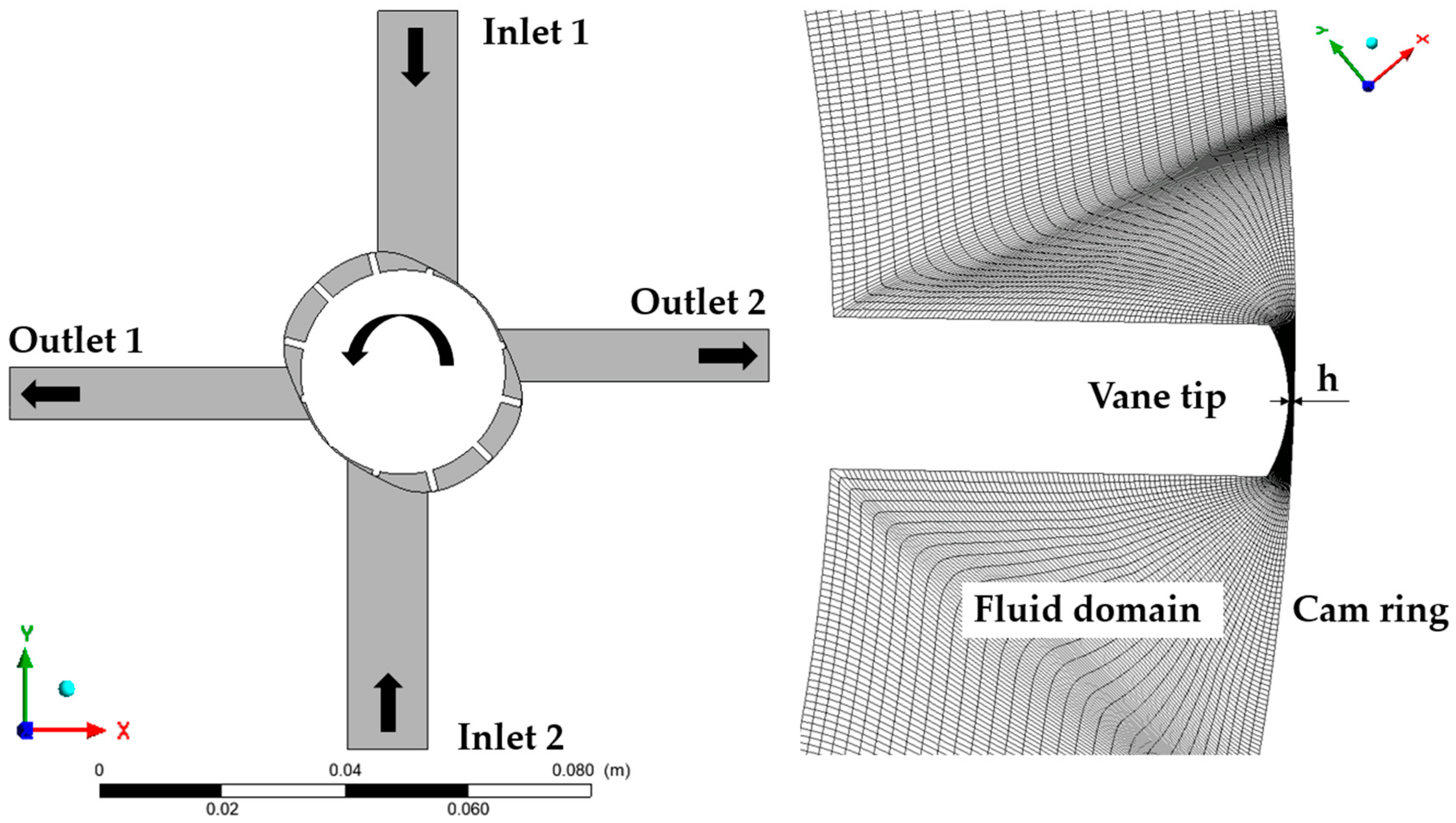
At first, a mesh convergence study on the 2D model was conducted. Therefore, the total cell count N in the rotor domain was altered between 64,900 and 234,000 cells. The stator meshes were kept constant with a sufficient fine resolution in the interface area towards the rotor. In Figure 6, the two possible directions to refine the rotor mesh are displayed. On the one hand, the cell number in the circumferential direction was increased by increasing the number of nodes on the cam ring and the number of nodes on the vane tips. By that, a refinement especially in the gap region was possible in the circumferential direction. On the other hand, the number of radial cells was altered. This change in the number of radial cell layers applied for the displacement chambers, as well as for the radial gaps between the vane tip and the cam ring, as the mesh had an O-topology. Because of that, an analysis focusing solely on the gap region was not possible, as the displacement chambers were simultaneously refined in the radial direction.

In a first step, seven different meshes were considered, where the mesh resolution was refined in both directions, isotropically. In Figure 7, the influence of the total cell count N on the evaluated volumetric efficiency ${\eta }_{vol}$ of the 2D vane pump can be observed.

It can be stated that an increase of the total cell count N led to higher predicted values for the volumetric efficiency of the pump. As the radial gaps were the only internal leakage paths where fluid could flow back from the delivery to the suction port, they completely prevailed the volumetric efficiency. In Figure 8a,b, the radial cell count $N_r,$ as well as the circumferential cell count on the vane tip $N_c,$ were altered independently.

Thus, the radial spatial resolution had a significant influence on the predicted volumetric efficiency. Yet, when a resolution of $N_r\geqq$ 40 cells was reached, the influence of further increasing the cell count decreased. For the circumferential resolution, a cell count of $N_c\geqq$ 14 cells seemed to be sufficient, as a further increase did not significantly alter the predicted volumetric efficiency anymore. This result was expected, since the leakage flows from one displacement chamber to the other were in the circumferential direction. Therefore, the developing circumferential velocity profile $u_{\phi }\left(r\right)$ in the gap between the vane tip and the cam ring prevailed the leakage mass flow. Hence, a good resolution in the radial direction was crucial.

When looking at the calculated instantaneous mass flow rates at outlet 1 while altering $N_c$ and $N_r$ independently in Figure 9a,b, a certain influence can be observed. Here, the influence of $N_r$ also seemed to be more significant than the influence of $N_c$.

For a rotating displacement pump, the transient pressure profile that developed inside a displacement chamber during one rotor revolution was distinctive. It was influenced by various variables like the internal pump geometry, the delivery pressure, and the rotational speed [25]. In Figure 10, this profile is plotted for a range of 0° to 180° shaft rotation angle. Since a balanced vane pump was investigated, this cycle repeated twice within one revolution of the pump rotor.

The pressure surge at about 41° rotation angle was caused by the compression of the displacement chamber before it connected to the delivery port. In this 2D case, because of the small available flow cross section, this pressure surge was much higher than in a 3D case.

When varying $N_c$ and $N_r,$ the resulting differences for the height of this pressure surge can be observed in Figure 11a,b. A significant influence of the height of the pressure surge on the spatial resolution is clearly visible. Finer resolutions tend to show a higher-pressure surge, while the energy is more likely dissipated when the resolution is lower. This also applies for the range of shaft rotation angles from 45° to 90°, when the displacement chamber was connected to the delivery port and therefore was pressurized. On this pressure plateau, pressure pulsations could be observed (see Figure 10). These resulted from other preceding or following displacement chambers connecting or disconnecting from the delivery port. The pressure pulsations traveled through the radial gaps and reached the observed displacement chamber. As the radial gaps were enlarged in this 2D case, this effect was even stronger than in a 3D case.

Based on this study, all further simulations were performed on a mesh with 42 radial cells and 21 circumferential cells on the vane tip. This led to a total cell count of 117,000 in the rotor area.

4.2. Time Step Size Influence

The influence of the time step size was investigated at 4000 rpm and 50-bar delivery pressure. To vary $\Delta t$, seven mesh sets with different angular step sizes $\Delta \phi$ were generated, as $\Delta t=\left(\Delta \phi ·60\right)/\left(2\pi ·n\right)$. They are listed in

Table 3. Correlation between angular resolution and time step size at 4000 rpm and legend for Figure 13.

	$\Delta \phi \mathbf{at} 4000 \mathbf{rpm} (°)$	Δt (s)	C (-)
A	1	$4.166·{10}^{-5}$	3.25
B	0.75	$3.125·{10}^{-5}$	2.45
C	0.5	$2.083·{10}^{-5}$	1.68
D	0.333	$1.388·{10}^{-5}$	1.16
E	0.25	$1.041·{10}^{-5}$	0.90
F	0.1667	$6.944·{10}^{-6}$	0.63

, together with the mean occurring Courant number C, which is defined in Equation (8):

$$C=\frac{u·\Delta t}{\Delta x}$$

(8)

Δx stands for the spatial resolution, which here is our smallest dimension of a computational cell. As ANSYS CFX is an implicit solver, the Courant–Friedrichs–Lewy condition $C\le 1$ does not need to be met in order to obtain a stable solution.

As can be obtained from Figure 12, there is nearly no influence of the time step size on the calculated volumetric efficiency. In Figure 13, it can be seen that the transient pressure ripple while the displacement chamber is connected to the delivery port is dependent on a sufficient temporal resolution.

Resulting from this analysis, all further calculations were performed with a maximum angular step size of 0.25°.

4.3. Internal Leakages

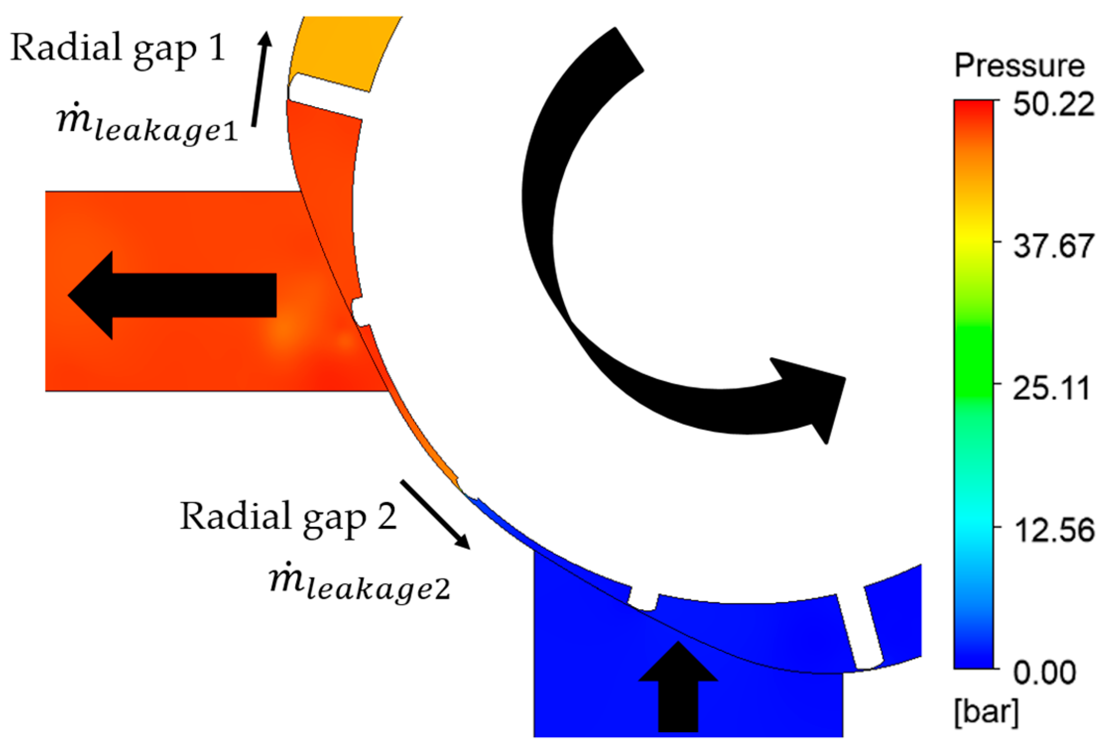
As already mentioned before, the radial gaps between the vane tips and the cam ring were the only leakage paths in this 2D case. To calculate the respective leakage mass flow rates through them, cross sectional planes normal to the circumferential direction which follow the mesh movement were defined at both radial gaps 1 and 2 in the vane middle axis (see Figure 3). The instantaneous mass flow rates passing through them were monitored. In Figure 14a,b, the influence of varying the delivery pressure and the rotational speed independently are displayed for the two defined leakage mass flows and the sum of both, which affect outlet 1. As the pump was symmetrical, it could be expected that at outlet 2 the same leakage mass flows could be observed. These mass flow rates were analyzed only at one specific angular position of a 30° shaft rotation angle.

When increasing the rotational speed while keeping the delivery pressure constant, the leakage mass flow 1, which was aligned against the direction of rotation, increased as the relative velocity between fluid and vanes increased. Contrary to that, leakage mass flow 2, which was aligned in the direction of rotation, decreased. In sum, the total leakage mass flow rate decreased while increasing the rotational speed up to 3000 rpm. By keeping the rotational speed constant while increasing the delivery pressure, both leakage mass flow rates and the sum increased as the driving pressure gradients increased.

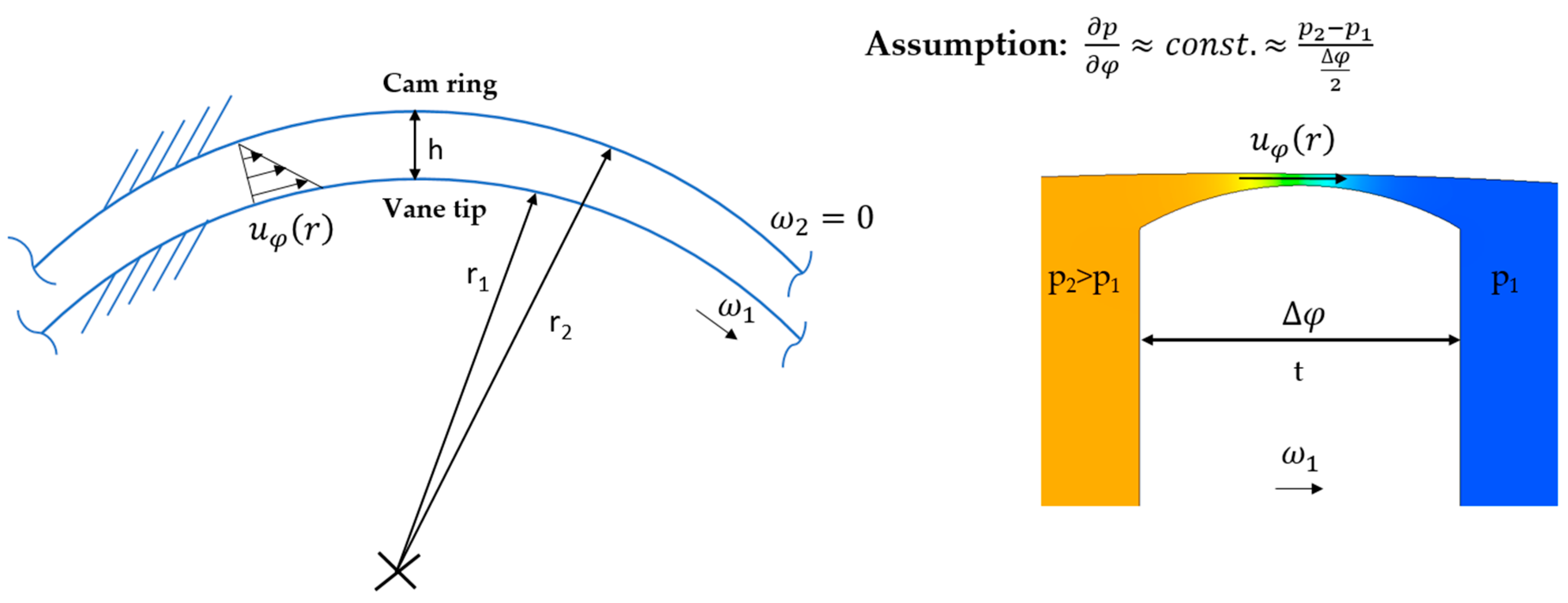
As already stated, the circumferential flow velocity profile in the radial gap prevailed the leakage mass flows through them. In Figure 15, the numerical results from the CFD simulations are compared with both analytical solutions for radial gap 1, which were analytically derived in Section 3. In this case, the mesh with 42 radial and 21 circumferential cells in the radial gap was used. For the derivation of the analytical solutions, $\frac{\partial p}{\partial \phi }=$7.79E9 Pa/rad was used. This value was obtained from the CFD simulations.

In Figure 15, it can be clearly seen that the numerical solution matches quite well to the analytically derived solution 1 (Equation (4)). The planar Couette–Poiseuille analytical solution 2 (Equation (7)) however led to a slight overprediction of the maximum speed. In this case, no kinetic energy was needed to counteract the centrifugal forces; therefore, the maximum velocity was higher.

As stated in the mesh convergence study, the leakages were strongly dependent on the radial resolution of the gaps. This could be verified by comparing the developing velocity profile in the gap with the analytical solution 1 for different radial cell counts $N_r$ in Figure 16.

When increasing the radial cell count $N_r$, the numerical solution approached analytical solution 1. Low cell numbers in the radial direction led to an overprediction of the occurring velocities in the radial gap and, thus, an overprediction of the leakage mass flow rates. This explained the lower predicted volumetric efficiencies in these cases. For a correct prediction of the leakages in this 2D case, a sufficient radial resolution was therefore necessary. In a 3D case, it may not be computationally feasible to use such a fine radial resolution. Furthermore, the immanent axial gaps provided another important leakage path in the 3D case, which was not taken into account in this work.

A variation of $N_c$ however showed nearly no influence on the developing circumferential velocity profile, as long as a value $N_c$≧ 14 was used.

4.4. Cavitation

With simulation setup 1, vapor cavitation was considered by applying a homogeneous Euler–Euler approach and incorporating the Rayleigh–Plesset cavitation model to describe the mass transfer between the vapor and the liquid oil.

4.4.1. General investigations

In Figure 17a,b, the resulting conveying characteristic and the volumetric efficiencies were plotted for different delivery pressures.

Up to 4500 rpm, the calculated actual volumetric flow rate $Q_{actual}$ followed the theoretical flow rate $Q_{theo}$ curve quite closely. With increasing rotational speed, the volumetric efficiency increased as the internal leakages decreased. The delivery pressure influence on the leakage flows was also clearly visible. At rotational speeds higher than 4500 rpm, vapor cavitation set in and the volumetric flow rate did not increase with the rotational speed anymore.

In Figure 18, the gas volume fraction of oil vapor is visualized for different rotational speeds at 5-bar delivery pressure.

It could be observed that vapor was generated when the low-pressure oil in the suction ports was filling the displacement chambers. Those areas of high gas volume fraction of vapor were conveyed with the chamber and persisted until reaching the pressurized delivery port. As condensation was a slower process than evaporation by two to three orders of magnitude, the vapor needed more time to condensate again. Increasing the rotational speed up to 8000 rpm, more and more vapor was generated in the suction ports; hence, no further increase of the volumetric flow rate was possible.

Besides the cavitation occurring at the suction ports, in the radial gaps vapor was also generated at higher rotational speeds.

This could be observed in the radial gaps where the pressure gradient was aligned against the direction of rotation. The occurring relative velocities were high and the static pressure dropped below the vapor pressure of oil, leading to vapor generation. In Figure 19, this is displayed for different rotational speeds at a delivery pressure of 5 bars. The cavitation in the radial gaps started to set in at $n>$ 6000 rpm. This was delayed compared to cavitation due to incomplete filling of the displacement chambers, which started already at $n>$ 4500 rpm.

In Figure 20, the volumetric efficiency is plotted as a function of the delivery pressure for different rotational speeds. At low speeds, the dependence of the volumetric efficiency on the delivery pressure was quite high. The delivery pressure dominated the leakage mass flows. When the rotational speed was increased, the contribution of the drag-induced flow in the gaps increased and the influence of the delivery pressure became smaller. Furthermore, when cavitation set in, there was almost no dependence of the volumetric efficiency on the delivery pressure visible anymore, as cavitation prevailed and limited the volumetric flow rate.

4.4.2. Influence of Suction Port Orientation

Since vapor is preferably generated at the suction ports, a design change of those was the first possibility to shift the cavitation onset to higher rotational speeds. To reduce the risk of a pressure drop below the vapor pressure of oil, the velocities occurring when the chamber is filled with fluid had to be reduced. Considering a nearly incompressible fluid, this led to the conclusion that the available cross section for the flow needed to be increased. The control times of the pump were fixed in order to prohibit a hydraulic short circuit of the pump, which would lead to even higher losses. Hence, the circumferential length of the suction ports could not be modified. In addition, the height of the 2D model was also fixed.

However, the orientation of the suction ports could be modified. Besides the perpendicular configuration, two other alignments were analyzed, which are displayed in Figure 21.

In Figure 22, the influence of the different suction port configurations can be clearly identified in the respective conveying characteristics. Tangential-oriented suction ports in the direction of rotation delayed the cavitation onset by about 500 rpm, in comparison to the perpendicular-oriented suction ports. Tangential oriented suction ports against the direction of rotation, however, led to a cavitation onset, which started 500 rpm earlier. This could be explained with the higher static pressure losses and velocities when the fluid had to be redirected into the displacement chamber by nearly 180°. In the cases where the fluid was flowing in the chambers tangentially in the direction of rotation, the occurring static pressure losses and velocities were the lowest. Therefore, cavitation started at higher rotational speeds.

It can be summarized that the employed two-phase homogeneous Euler–Euler model was capable of capturing the basic cavitation phenomena using the Rayleigh–Plesset cavitation model. However, the release of dissolved air, which was also always present in the hydraulic oil circuit and presented another important mechanism to reduce the volumetric flow rates at high rotational speeds, was not incorporated in this method.

4.5. Free Air at the Inlets (IGVF)

In the second simulation setup, the effects of an introduced IGVF of free air bubbles were analyzed. At first, the influence of the applied modeling approach needed to be investigated. Again, a Euler–Euler approach was used, as presented in Table 2. This meant one pressure field was shared by both phases. In using the homogenous approach, the same assumptions were made for the velocity and temperature field. When the inhomogeneous approach was applied, two sets of momentum, energy, and mass conservation equations were solved. It was a valid assumption to use the homogeneous approach, if occurring slip velocities between the two phases were small. In this setup, a continuous oil phase and a disperse phase of air bubbles was applied. It was assumed that the air bubbles had a mean diameter of $d_{mean}$= 0.1 mm. This was an observation from experiments with real transmission systems. Of course, this assumption significantly influenced the results, as the interface area was responsible for the interphase interactions in the flow. For this mean bubble diameter and the occurring speeds in this 2D case, the use of a homogeneous approach was valid according to [26], as the occurring relative velocities should be small. However, for higher rotational speeds and larger mean diameters the homogenous assumption might not have been correct anymore. To investigate this further, a study examining the results of both multiphase approaches for a mean bubble diameter of 0.1 mm was conducted.

In the instantaneous plots of the pressure in the displacement chamber shown in Figure 23a–c, significant differences are visible between both approaches. These differences were especially apparent at a low IGVF of 5% and a high IGVF of 40%. At 20% IGVF, the difference between both curves was insignificant.

This observation could also be made for the instantaneous outlet mass flow rates. However, in the time averaged mass flow rates and the volumetric efficiencies, no significant differences were noticeable between either approach. As the instantaneous pressure and mass flow rate curves were important characteristics to asses a pump, it was decided to only use the inhomogeneous approach in all further simulations. This was possible with a reasonable computational time in this simple 2D case.

The assumption for the mean air bubble diameter $d_{mean}$ was another significant model parameter in this setup. In Figure 24a,b, its influence on the instantaneous mass flow rate and the pressure at outlet 1 is shown.

Increased interphase momentum interactions led to significant differences when the mean bubble diameter was increased from 0.1 to 0.3 mm. There was no significant difference visible when decreasing the mean diameter from 0.1 to 0.01 mm.

However, it could be demonstrated that it was crucial to check the assumption of the bubble mean diameter concerning its validity, as it heavily influenced the results. All following simulations were conducted with a mean air bubble diameter of $d_{mean}$= 0.1 mm.

In Figure 25a,b, the obtained conveying characteristic and the volumetric efficiencies of the 2D pump with different IGVF are displayed.

The simulations were performed for rotational speeds up to 4000 rpm. With an IGVF > 0, the compressibility of the mixture was much higher than that with IGVF = 0. This led to a lower volumetric flow rate and of course volumetric efficiency than with pure oil. With increasing IGVF, the volumetric efficiency continued to decrease even more and stayed below the value of ${\eta }_{vol}<1-\mathrm{IGVF}$. It was also interesting that with an IGVF > 0, the volumetric efficiency slightly decreased while increasing the rotational speed from 1000 up to 4000 rpm. With pure oil, it slightly increased, as already discussed in Section 4.3 and Section 4.4. To further investigate this effect, the leakage mass flow rates through the radial gaps had to be analyzed again while varying the IGVF. This is again evaluated for one specific time step at a shaft rotation angle of 30°, as displayed in Figure 3.

It is clearly visible in Figure 26a,b, that in radial gap 1, an IGVF > 0 led to significantly higher leakage mass flow rates. This was because of the high compressibility of the mixture. The volume decrease of the displacement chamber did not lead to such a high-pressure raise as with pure oil. Therefore, the occurring pressure gradient from the enclosed displacement chamber to the delivery port in the radial gap was much higher with an IGVF > 0 than with pure oil. This effect led to higher leakage mass flow rates in radial gap 1. In radial gap 2, higher leakage mass flow rates were also observable with an IGVF > 0. Because of the low delivery pressure of 5 bars, the sign of the leakage mass flow rate even became negative at higher rotational speeds. This meant the leakage mass flow was beneficial and fluid flowed back into the delivery port. This beneficial leakage was reduced with an IGVF > 0 as the mixture density was reduced, which also led to lower inertia forces. Hence, with approximately similar pressure gradients in the gap, the drag-induced amount of the leakage mass flow was smaller compared to the pressure gradient-induced amount. Therefore, the detrimental leakage was higher at low rotational speeds and the beneficial leakage was smaller at higher rotational speeds. At 40% IGVF, no sign change into a beneficial leakage could be observed at radial gap 2, as the pressure gradient-induced leakage flow amount prevailed over the drag-induced amount because of the low mixture density.

In Figure 27, the effects of different IGVF on the instantaneous displacement chamber pressure profile are shown. The volume decrease of the displacement chamber with IGVF = 0 led to a high-pressure surge up to 80 bars, caused by the low compressibility of pure oil (the peak is cut away in the Figure to achieve a better perceptibility of the other curves with an IGVF > 0). With an IGVF > 0, this pressure surge was significantly and increasingly reduced because of the rising compressibility of the mixture. Additionally, the pressure surge was delayed while increasing the IGVF.

It was also apparent that the occurring pressure ripple while the displacement chamber was connected to the delivery port was much higher with an IGVF > 0 than with pure oil. This can also be observed in Figure 27, and is presumably caused by the rising compressibility gradients in the mixture.

At the instantaneous pressure profiles at the outlets, the influence of an IGVF > 0 is also clearly visible in Figure 28a,b. At 1000 rpm the differences were not that apparent, but it is obvious that with an IGVF > 0 there were higher pressure ripples occurring. At 4000 rpm, a high-pressure surge in the curve for an IGVF = 0 was visible. This pressure surge resulted from a displacement chamber connecting to the delivery port, and the respective pressure waves were transported to the outlet with the speed of sound. It appeared at a 30° rotation angle interval as the pump consisted of twelve vanes. These pressure surges were damped with an IGVF > 0. Furthermore, it could be observed that they arrived at the outlet later in time, as the IGVF was increased. This was due to a significantly reduced speed of sound in a mixture of oil and air compared to pure oil [27]. Overall, the outlet pressure ripple was reduced with an IGVF > 0 at higher rotational speeds. At lower rotational speeds, it was increased.

Looking at the instantaneous mass flow rates at outlet 1 in Figure 29a,b, an increased flow ripple is apparent for an IGVF > 0 for both 500 rpm and 2000 rpm. For the highest considered IGVFs of 20% and 40% even intermittent backflow can be observed at the outlet.

In Figure 30, the air volume fraction distribution in an enclosed displacement chamber is displayed. The highest volume fractions of air are conveyed near the rotor wall, since the lowest static pressure values can be found there.

Besides pressure ripple, mass flow ripple, and volumetric efficiency, power demand was also an important characteristic of hydraulic pumps. For pure oil, one can identify a high increase in power demand from the 0° to 15° rotation angle in Figure 31a,b. Here, the compression of the displacement chamber began before it connected to the delivery port. The compressibility of pure oil was quite low. Therefore, the torque and power demand to compress the liquid was quite high. With an IGVF > 0, the power demand decreased significantly, as the compressibility of the mixture was significantly higher. At 500 rpm, the peak of the power demand decreased by 45% with a 5% IGVF. Further increasing the IGVF to 10% led to another decrease of power demand. IGVFs of 20% and 40% did not further lower the power demand anymore. At a higher rotational speed of 4000 rpm, 5% IGVF reduced the power demand peak by about 70%, while a further increase in IGVF > 5% did not lead to another decrease in power demand for the compression. This was due to higher acting inertia forces at 4000 rpm, which supported the compression.

Furthermore, it could be observed that the peak of the power demand appeared later in time and at correspondingly higher rotation angles, while the IGVF increased. The increasing mixture compressibility delayed the pressure rise, as it could also be observed in the displacement chamber pressure curves. Overall, it can be stated that an IGVF > 0 reduced the average power demand of the pump significantly. Of course, this came at the cost of a significant loss of volumetric efficiency and flow rate.

5. Conclusions

A two-dimensional CFD study of a balanced vane pump was presented in this paper. Within the scope of a mesh convergence study, the influence of the spatial resolution of the radial gaps was assessed. It could be shown that especially the mesh resolution in the radial direction in the gap region was crucial for reproducing a correct circumferential leakage flow velocity profile and therefore achieving a good prediction of the volumetric efficiency of the pump. However, the influence of the radial gaps was exaggerated in this considered 2D case compared to a real 3D pump, as the axial gaps were missing and the radial gaps presented the only leakage paths. Additionally, they had to be enlarged in height because of numerical issues.

In a first simulation setup, the characteristics of the pump concerning vapor cavitation were analyzed by using the Rayleigh–Plesset cavitation model with a homogeneous Euler–Euler two-phase approach. Vapor generation could be observed in the suction area, where the displacement chambers were filled. Beginning at 4500 rpm, cavitation set in and declined a further rise of outlet volumetric flow rate with an increasing rotational speed. To optimize this, two other suction port configurations were analyzed with the result that a tangential alignment of the suction ports in the direction of rotation led to a delay of the cavitation onset compared to the perpendicular alignment by about 500 rpm. Besides that, in the radial gaps, cavitation could also be detected at rotational speeds greater than 6000 rpm.

In a second two-phase flow Euler–Euler simulation setup, the influence of different inlet gas volume fractions of free air was investigated. It could be shown that the employed modeling approach for phase interaction, as well as interface area, had great influence on the instantaneous pressure and mass flow rate curves. For an assumed mean air bubble diameter of 0.1 mm and an inhomogeneous multiphase approach, inlet gas volume fractions between 5% and 40% were investigated. This setup was capable of predicting the drop in volumetric efficiency, which appeared when an IGVF > 0 was present. Through the increased compressibility of the mixture, the volumetric flow rate was reduced. Besides that, the developing pressure field with an IGVF > 0 led to partly higher leakage mass flow rates through the radial gaps than with an IGVF = 0. The occurring pressure surges, when a displacement chamber connected to the delivery ports, were damped because of the high compressibility of air. This meant that especially at rotational speeds higher than 2000 rpm, this effect led to lower peaks in the pressure ripple at the outlets. At rotational speeds lower than 2000 rpm, an IGVF of air > 0 led to higher pressure ripple. However, it could be predicted that for all considered rotational speeds, the outlet mass flow rate ripple significantly increased with an IGVF > 0. For an IGVF ≧ 20%, even intermittent backflow could be observed. In multiphase operating conditions, the highest volume fractions of air were conveyed along the rotor wall, which was similar to the multiphase pumping behavior of centrifugal pumps. Furthermore, it was found that introducing an IGVF of air reduced the mean power demand of the pump significantly, compared to a single-phase operation.

Overall, with the presented 2D vane pump model, all relevant multiphase flow phenomena could be reproduced. However, when dealing with an IGVF of free air, the employed multiphase modeling approach, as well as the assumptions for the mean bubble diameter, influenced the results strongly. The requirements concerning the mesh quality were very high and for radial gap heights smaller than 50 µm and rotational speeds higher than 4000 rpm, convergence could not be obtained. The use of this modeling approach in real 3D cases, however, leads to high total cell counts and therefore a high computational effort.

References

1. Ivantysyn, J.; Ivantysynova, M. Hydrostatische Pumpen und Motoren, 1st ed; Vogel Verlag: Wuerzburg, Germany, 1993; pp. 123, 358–361. [Google Scholar]
2. Inaguma, Y.; Yoshida, N. Variation in Driving Torque and Vane Friction Torque in a Balanced Vane Pump. SAE Tech. Paper 2014. [Google Scholar] [CrossRef]
3. Will, D.; Gebhardt, N. Hydraulik: Grundlagen, Komponenten, Systeme, 6th ed.; Springer: Berlin, Germany, 2014; pp. 132–134. [Google Scholar]
4. Giuffrida, A.; Lanzafame, R. Cam shape and flow rate in balanced vane pumps. Mech. Mach. Theory 2005, 40, 353–369. [Google Scholar] [CrossRef]
5. Inaguma, Y. Theoretical Analysis of Mechanical Efficiency in Vane Pump. JTEKT Eng. J. 2010, 1007E, 28–35. [Google Scholar]
6. Zouani, A.; Dziubinschi, G.; Marri, V. Optimal Vanes Spacing for Improved NVH Performance of Variable Displacement Oil Pumps. SAE Tech. Paper 2017. [Google Scholar] [CrossRef]
7. Inaguma, Y.; Yoshida, N. Small High-Efficiency Vane Pump Based on Vane Pump Theory. SAE Int. J. Passeng. Cars-Mech. Syst. 2015, 8, 614–623. [Google Scholar] [CrossRef]
8. Battarra, M.; Blum, A.; Mucchi, E. Kinematics of a balanced vane pump with circular tip vanes. Mech. Mach. Theory 2019, 137, 355–373. [Google Scholar] [CrossRef]
9. Battarra, M.; Mucchi, E. On the relation between vane geometry and theoretical flow ripple in balanced vane pumps. Mech. Mach. Theory 2020, 146, 103736. [Google Scholar] [CrossRef]
10. Lu, Y.; Zhang, W.; Zhao, Y.-Y.; Wang, Z.-Z.; Shu, P.-C. Studies on several key problems of water hydraulic vane pump. Ind. Lubr. Tribol. 2011, 63, 134–141. [Google Scholar] [CrossRef]
11. Fornarelli, F.; Lippolis, A.; Oresta, P.; Posa, A. Investigation of a pressure compensated vane pump. Energy Procedia 2018, 148, 194–201. [Google Scholar] [CrossRef]
12. Truong, B.N.; Quang Truong, D.; Thanh Trung, N.; Kwan, A.K. Mathematical modeling of a variable displacement vane pump for engine lubrication. Int. Conf. Control Autom. Syst. (ICCAS) 2015, 15, 1946–1951. [Google Scholar]
13. Bianchi, G.; Fatigati, F.; Murgia, S.; Cipollone, R. Design and analysis of a sliding vane pump for waste heat to power conversion systems using organic fluids. Appl. Therm. Eng. 2017, 124, 1038–1048. [Google Scholar] [CrossRef]
14. Rundo, M.; Altare, G.; Casoli, P. Simulation of the Filling Capability in Vane Pumps. Energies 2019, 10, 283. [Google Scholar] [CrossRef] [Green Version]
15. Chen, Z.; Wang, J.; Cui, S.; Feng, H.; Sha, R. Numerical simulation and design methodology of a novel asymmetric cylinder profile for sliding vane vacuum pumps. Vacuum 2019, 169, 108945. [Google Scholar] [CrossRef]
16. Suzuki, K.; Nakamura, Y.; Yakabe, S.; Watanabe, H.; Nakamura, K. Characteristics Prediction of Vane Pump by CFD Analysis. KYB Tech. Rev. Technol. 2016, 53, 8–15. [Google Scholar]
17. Hong, S.; Son, G. Numerical study of a vane vacuum pump with two-phase flows. J. Mech. Sci. Technol. 2017, 31, 3329–3335. [Google Scholar] [CrossRef]
18. Bianchi, G.; Rane, S.; Kovacevic, A.; Cipollone, R. Deforming grid generation for numerical simulations of fluid dynamics in sliding vane rotary machines. Adv. Eng. Softw. 2017, 112, 180–191. [Google Scholar] [CrossRef]
19. Iannetti, A.; Stickland, M.T.; Dempster, W.M. A CFD and experimental study on cavitation in positive displacement pumps: Benefits and drawbacks of the ‘full’ cavitation model. Eng. Appl. Comput. Fluid Mech. 2016, 10, 57–71. [Google Scholar] [CrossRef] [Green Version]
20. Suh, J.-W.; Kim, J.-H.; Kim, J.-W.; Choi, Y.-S.; Joo, W.-G.; Lee, K.-Y. Development of numerical Eulerian-Eulerian models for simulating multiphase pumps. J. Pet. Sci. Eng. 2018, 162, 588–601. [Google Scholar] [CrossRef]
21. Patil, A. Performance Evaluation and CFD Simulation of Multiphase Twin-Screw Pumps. Ph.D. Thesis, Texas A & M University, College Station, TX, USA, 2013. [Google Scholar]
22. Hesse, J.; Spille-Kohoff, A.; Hauser, J.; Schulze-Beckinghausen, P. Structured meshes and reliable CFD simulations: TwinMesh for positive displacement machines. VDI-Berichte 2014, 2228, 297–308. [Google Scholar]
23. Bakir, F.; Rey, R.; Gerber, A.G.; Belamri, T.; Hutchinson, B. Numerical and experimental investigations of the cavitating behavior of an inducer. Int. J. Rotating Mach. 2004, 10, 15–25. [Google Scholar] [CrossRef] [Green Version]
24. Schlichting, H.; Gersten, K. Grenzschicht-Theorie, 10th ed.; Springer: Berlin, Germany, 2006; pp. 101–104. [Google Scholar]
25. Sullivan, P.E.; Sehmby, M. Internal Force Analysis of a Variable Displacement Vane Pump. In Proceedings of the SAE 2012 World Congress & Exhibition, Detroit, MI, USA, 24–26 April 2012. [Google Scholar]
26. Brennen, C.E. Fundamentals of Multiphase Flow, 1st ed.; Cambridge University Press: Cambridge, UK, 2005; pp. 78–79. [Google Scholar]
27. Kieffer, S.W. Sound Speed in Liquid-Gas Mixtures: Water and Water-Steam. J. Geophys. Res. 1977, 82, 2895–2904. [Google Scholar] [CrossRef]
Figure 1. Inner parts of a balanced vane pump consisting of the rotor, twelve vanes, and the cam ring.
Energies 13 03314 g001
Figure 2. 2D vane pump model and meshing details of the rotor.
Energies 13 03314 g002
Figure 3. Internal leakage paths from outlet 1 to inlets 1 and 2 at 30° shaft rotation angle.
Energies 13 03314 g003
Figure 4. Simplified model 1 to obtain an analytical solution for u φ ( r ) in the radial gap.
Energies 13 03314 g004
Figure 5. Simplified model 2 to obtain an analytical solution for u φ ( r ) in the radial gap, which is here approximated by u x ( y ) .
Energies 13 03314 g005
Figure 6. Meshing parameters in the radial gap region.
Energies 13 03314 g006
Figure 7. Dependence of the volumetric efficiency on the total cell count N in the rotor region.
Energies 13 03314 g007
Figure 8. Influence of (a) N r at N c = 31 and (b) N c at N r = 42 on the volumetric efficiency.
Energies 13 03314 g008
Figure 9. Influence of (a) N r at N c = 31 and (b) N c at N r = 24 on the instantaneous mass flow rate ripple at outlet 1.
Energies 13 03314 g009
Figure 10. Instantaneous displacement chamber pressure curve for half a revolution at 50-bar delivery pressure and 4000 rpm.
Energies 13 03314 g010
Figure 11. Influence of (a) N r at N c = 31 and (b) N c at N r = 24 on the pressure surge when the displacement chamber connects to the delivery port.
Energies 13 03314 g011
Figure 12. Time step influence on the volumetric efficiency.
Energies 13 03314 g012
Figure 13. Influence of the time step size on the displacement chamber pressure ripple while the chamber is connected to the delivery port.
Energies 13 03314 g013
Figure 14. Leakage mass flows through the radial gaps under (a) variation of the rotational speed at a delivery pressure of 10 bars (b) variation of the delivery pressure at a rotational speed of 1000 rpm.
Energies 13 03314 g014
Figure 15. Comparison of the two analytically derived circumferential velocity profiles with the numerical solution at 10-bar delivery pressure and a rotational speed of 4000 rpm in the radial gap 1.
Energies 13 03314 g015
Figure 16. Comparison of the numerical results with different N r   with the analytical solution 1 in the radial gap 2 at   N c = 31 , 4000 rpm and 50-bar delivery pressure.
Energies 13 03314 g016
Figure 17. (a) Actual volumetric flow rate of the analyzed 2D pump and (b) volumetric efficiencies considering vapor cavitation at different delivery pressures and rotational speeds.
Energies 13 03314 g017
Figure 18. Development of the vapor gas volume fraction distribution at 5-bar delivery pressure for different rotational speeds.
Energies 13 03314 g018
Figure 19. Development of the vapor gas volume fraction distribution focusing on radial gap 1 at 5-bar delivery pressure for different rotational speeds.
Energies 13 03314 g019
Figure 20. Dependence of the volumetric efficiency on the delivery pressure for different rotational speeds.
Energies 13 03314 g020
Figure 21. Overview of the analyzed suction port configurations.
Energies 13 03314 g021
Figure 22. Actual volumetric flow rates of the different suction port configurations at 5-bar delivery pressure.
Energies 13 03314 g022
Figure 23. Difference between homogeneous and inhomogeneous multiphase approach for the instantaneous displacement chamber pressure ripple at 5-bar delivery pressure and 2000 rpm at (a) inlet gas volume fraction (IGVF) = 5%, (b) IGVF = 20%, and (c) IGVF = 40%.
Energies 13 03314 g023
Figure 24. Influence of the mean bubble diameter d m e a n on the (a) outlet 1 mass flow rate and (b) outlet 1 pressure ripple at 5-bar delivery pressure and 2000 rpm.
Energies 13 03314 g024
Figure 25. (a) Volumetric flow rates and (b) the respective volumetric efficiencies for different IGVF of free air and rotational speeds at 5-bar delivery pressure.
Energies 13 03314 g025
Figure 26. Leakage mass flow rates in (a) radial gap 1 and (b) radial gap 2 for different IGVF of free air and rotational speeds at 5-bar delivery pressure.
Energies 13 03314 g026
Figure 27. Instantaneous displacement chamber pressure profiles for different IGVF of free air at 5-bar delivery pressure and 2000 rpm.
Energies 13 03314 g027
Figure 28. Influence of the IGVF of free air on the outlet 1 pressure ripple at 5-bar delivery pressure, (a) 1000 rpm and (b) 4000 rpm.
Energies 13 03314 g028
Figure 29. Influence of the IGVF of free air on the instantaneous outlet 1 mass flow rate at 5 bars, (a) 500 rpm and (b) 2000 rpm.
Energies 13 03314 g029
Figure 30. Free air gas volume fraction distribution for a single displacement chamber at 5 bars, 2000 rpm and an IGVF of 40%.
Energies 13 03314 g030
Figure 31. Influence of the IGVF of free air on the instantaneous power demand at 5-bar delivery pressure, (a) 500 and (b) 4000 rpm.
Energies 13 03314 g031