Article

Methodology for Energy Efficiency on Lighting and Air Conditioning Systems in Buildings Using a Multi-Objective Optimization Algorithm

by
Suzane A. Monteiro
1,2,*,
Flávia P. Monteiro
1,
Maria E. L. Tostes
2 and
Carminda M. Carvalho
2
1
Campus Oriximiná, Federal University of Western Para (UFOPA), Oriximiná 68270000, Brazil
2
Electrical Engineering Department, Federal University of Para (UFPA), Belém 66075-110, Brazil
*
Author to whom correspondence should be addressed.
Energies 2020, 13(13), 3303; https://doi.org/10.3390/en13133303
Submission received: 3 June 2020 / Revised: 23 June 2020 / Accepted: 24 June 2020 / Published: 28 June 2020

Abstract

:
The purpose of this article is to develop a methodology to apply to multi-objective optimization algorithms aimed at energy efficiency in buildings, considering aspects such as incremental cost, energy consumption, greenhouse gas emissions and energy efficiency levels of lighting and air conditioning system, according to the mandatory technical regulation in public buildings in Brazil. Presenting a solution to assist in the decision making of engineers, architects or building managers for the optimal arrangements’ choice for lighting and air conditioning equipment, considering each built environment and project profile. For the validation process, a basic building was created with 15 rooms spread over three floors, according to the most common construction parameters in the North of Brazil. First, different combinations of objective-function candidates were investigated to compose the multi-objective algorithm fitness function, analyzing its performance in two central scenarios: (1) adding some “baits” in air conditioning equipment files, and (2) without this inclusion. Thus, it was found that considering only three objective functions—incremental cost, energy consumption and the air conditioning energy efficiency coefficient—it is possible to get optimal non-dominated solutions in both scenarios, thus highlighting the robustness of the proposed methodology.

1. Introduction

Along with humanity’s progress, there are social, economic and environmental problems. The connection between these topics is clear, since economic development entails social and environmental impacts both locally and globally. The solution to this problem is to invest in practices based on sustainable development to use raw materials and, at the same time, reduce our impact on the environment as much as possible. However, the first step towards achieving sustainability is to improve our relationship with energy. All energy aspects are important, from generation to final use by the consumer.
One way to contribute to these challenges is through the continuous monitoring of each category individually, by sector and end use of energy, to prepare specific and more assertive energy efficiency measures. At this stage, it is intuitive to think directly in the industrial sector, as a major consumer of electricity and raw materials, but special attention should be given to constructions and buildings.
The constructions and building sector is one of the most heavily dependent on natural resources, consuming about 16% of the water supply, 25% of wood and 40% of fossil fuels and their manufactured materials around the world [1,2,3]. According to the report of the United Nations Environment Program (UNEP), Sustainable Building and Climate Initiative (SBCI), published in March 2007, the impact of measures concerning efficient architecture and energy saving in buildings to combat global warming would be greater than the impact of all greenhouse gas emission restrictions set out in the Kyoto Protocol.
This report recommended the more efficient use of concrete, metals and wood in construction, beyond decreasing energy consumption in items such air conditioning equipment and lighting systems in homes and offices. This would bring savings of billions of dollars yearly, since this sector alone accounts for about 40% of the world’s electricity consumption.
In Brazil, buildings make up 51.1% of the electricity consumed annually, according to BEN 2019 (National Energy Balance—Base Year 2018) shown in Figure 1. The Brazilian residential sector consumed 25.6% of electricity from the national energy matrix, the commercial sector, 17.2%, and public, 8.3%, where much of this energy goes to the air conditioners and lamps of such establishments [4].
Therefore, it is essential to work on measures to constantly refine the buildings energy performance. The right decisions in the project phase can produce lower energy consumption construction and greater sustainability, also. However, the question remains: where to invest?
Subsequently, several concepts, classifications and norms for efficient buildings appeared, such as Zero Energy Building (ZEB), Nearly Zero Energy Building (NZEB) and Zero Carbon Building (ZCB). ZEB buildings are those whose total amount of energy consumed annually is approximately equal to the renewable energy produced on site (Net Zero Site Energy) or from external renewable energy sources (Net Zero Source Energy). Following the same idea, NZEB buildings follow a buildings energy performance European standard that recognizes those with high energy efficiency associated with renewable energy sources, but consumption slightly higher than energy produced, forming a close to zero annual energy balance.
Observing some problems in the conceptualization of ZEB and NZEB, researchers proposed the ZCB, which emphasizes the quality and not the quantity of the energy produced. Buildings classified as ZCB must have zero energy balance, integrating a zero balance in CO2 emissions, through efficient and sustainable energy management techniques.
In Brazil, in 1985, Federal Government created the National Electricity Conservation Program, attached to the Ministry of Mines and Energy and executed by Eletrobras. The principal aim of this program was to articulate the electricity sector and society, promoting energy efficiency and the rational use of energy in Brazil. As a product of this initiative, the equipment labeling program and, subsequently, the building labeling program, PROCEL Edifica, was born. In 2009, within PROCEL Edifica building labeling, the Technical Quality Regulation for the Energy Efficiency Level of Commercial, Service and Public Buildings (RTQ-C [5]) and the Technical Quality Regulation for the Energy Efficiency Level of Residential Buildings (RTQ-R) and their complementary documents were created.
The RTQ-C assesses the crucial aspects of a building: envelope, systems of lighting, air conditioning, water heating, estimated consumption of basic equipment, rational use of water, local generation of renewable energy and carbon dioxide emissions. However, the label is not mandatory for all categories, only in the federal level public sector in the case of new construction or retrofit, but the tendency is a gradual extension to others, reaching the residential sector.
In this context, it raises the proposed methodology based on multi-objective optimization algorithms for building efficiency, focus on its air conditioning and lighting systems. First, the user sets artificially lit and cooled environments characteristics. Thereafter, the algorithm realizes ac luminotechnical and thermal capacity calculation for each room. Then, its results become the best arrangement of lamps and air conditioning units reaching from an input file by room, and other important energy and costs information about it, also.
The algorithm aim is to assist in the decision making of managers, engineers and architects, finding an optimal sequence of devices by room according to the candidate objective function seen as the most important for their project: (1) incremental costs with the purchase of this equipment; (2) energy consumption and, the associated greenhouse gases and their energy cost; (3) lighting system energy efficiency level; and (4) air conditioning system energy efficiency level. To calculate the building’s energy performance, a recent version of the RTQ-C (in the validation stage) guidelines was used: the Brazilian technical regulation. Testing both performance and robustness, the algorithm will be applied in a model building, in a controlled scenario.

2. Related Works

To assist in the development of the proposed methodology, beyond revealing the circumstances and provide greater understanding of the issue, it was fundamental to research the state of the art of software and algorithms about building energy efficiency and environmental comfort. The study of energy efficiency and environmental comfort in buildings is comprehensive, including: envelope, air conditioning system, environment or water heating system, lighting, renewable energy sources, optimal use of water, among others.

2.1. Envelope

Envelope optimization is a very complex subject, because it relates many variables. To contribute to the solution for this problem, article [6] proposes to introduce a new optimization algorithm based on simulation to minimize the liquid thermal load of the buildings, considering ten parameters, including the ratio between the window and the wall, the orientation of the building, roof material and wall material. The objective-function of this genetic algorithm represents the hourly thermal load average of the building (for one year), with the total area of the window as a constraint.
Bingham, Agelin-Chaab and Rosen [7] applied a Non-dominated Sorting Genetic Algorithm (NSGA-II) multi-objective optimization to achieve the best envelope characteristics, aiming improve residential buildings energy performance located in the Bahamas. Their methodology acts on building energy consumption and life cycle using the combination of jEPlus + EA and EnergyPlus simulation. The results showed energy reductions from current standards, reaching up 39%, decreasing lifecycle cost up to 18.5%.
Another envelope optimization initiative was recorded by in [8], where a genetic algorithm mono-objective was developed to optimize an environmentally friendly building projected by BIM technology, seeking to find a greater combination of construction material that produces an OTTV (General Thermal Transfer Value) and an envelope energy performance indicator closest to the ideal as possible. The initial result showed that the genetic algorithm could find an ideal combination of materials with a reduced OTTV of 16%.
Focusing on incremental cost analysis, [9] talks about energy consumption prediction through 18 parameters of envelope performance using artificial neural networks. The methodology employed DeST (Designer’s Simulation Toolkit) and MATLAB ANN (Artificial Neural Networks) toolbox, expecting building materials combinations as algorithm response to achieve optimal energy efficiency and reduce incremental cost.
Liu, Yu and Qi [10] aim to apply a fuzzy Analytic Hierarchy Process (AHP) model to the optimization of building material in an actual controlled scenario for the rapid and reliable completion of the procedure. In this experiment, three different sustainable building materials (composite bricks, silt bricks, building rubble) were evaluated by three indices (adaptability, economy and progress) and 14 sub-indices (energy use, energy cost, transport cost, durability, fire, insulation performance, among others). Each material received a score of specialists per sub-index, which was assigned a weight.
These works were very relevant to energy efficiency in buildings. However, these assess only one face of the problem at a time: thermal load, energy consumption, energy performance indicator or incremental cost.

2.2. Control and Automation

Optimization in buildings automation is another pertinent subject in terms of energy efficiency and environmental comfort in buildings. A building management system or building automation controls some of the most used systems in building, sometimes all of them together, unifying mechanics e/or electrics elements and forming an intelligent building. Therefore, as many automation and control systems are disponible in the market and also various controllable machines, the main challenge in this area is the integration and communication of all modules.
Chandrasekara et al. [11] discuss about automation and control systems to implement both user comfort and energy consumption. Oezluek [12] expounds a generic framework designed to solve project complex problems of building automation system with several organisms of control and, consequently, different set points and protocols.
Fanti et al. [13] work on a strategy in buildings ventilation automation for harnessing the natural wind reducing energy consumption and providing thermal comfort. Applying TRNFLOW and a particle swarm optimization algorithm together, the proposed strategy optimized window opening dynamically in a residential building in the Mediterranean climatic context.
Martirano et al. [14] presented another solution involving building automation systems. Using fuzzy logic, they sought to optimize energy performance and environmental comfort of an office in different scenarios regarding the solar energy and automation systems in air conditioning and lighting systems, beyond control over curtains with dynamic shading.
A bottleneck to be pointed out in the solutions proposed by the aforementioned articles was the non-inclusion of the building design stage, besides not considering, for example, reductions in incremental cost and impact on the environment by the actions developed.

2.3. Heating and Air Conditioning

Heating, cooling and air conditioning systems optimization contributes to a considerable percentage of the building energy consumption, about 50%. This justifies their importance and impact on the energy efficiency. Indoor conditions are affected by static and dynamic factors. Static factors could be architecture, orientation of rooms and windows size, and dynamic factors, the external climate and the number of occupants in the room.
Liu et al. [15] projected a central system to control and to optimize an air conditioning system of chilly water circulation developed on the LabVIEW software. Varying the chilled water temperature and flow, authors verified the air conditioning system optimal set points and attributes of operation in an office building.
Fan et al. [16] worked on a measure to increment intelligent buildings to self-adjust independent the season through a strategy for managing air conditioning load optimization with a software and wireless. The main objective of the action is to smooth the load curve and peak load detachment with just two levels: summer and winter.
Part of the improvement of an air conditioning system depends on its monitoring. Zhou, Yan and Lin [17] describe an online monitoring technology for the energy efficiency of a central air-conditioning system (water cooling) in real time by adjusting the supply temperature of cold water, cooling water flow, cooling tower airflow, and regulatory equipment operating units.
To achieve good thermal comfort in the countries closest to the poles, it is also essential to work on ambient heating. Javed et al. [18] proposed a process of radiator environmental heating system optimization applied in a residential building to calculate the ideal flow rate of those radiators to maintain a living room. Three different optimization processes were employed, evaluating particle swarm optimization algorithm (PSO), genetic algorithm (GA) and sequential quadratic programming optimization algorithm (SQP) with the modeled building through a recurrent neural network. To measure the performance of the techniques, the mean square error (MSE) was used and found a rate of 38.87% smaller compering PSO to GA and 21.19%, compering PSO to SQP.
It is interesting to mention that the studies on air conditioning mentioned above focused only on the operating characteristics of these systems through the efficiency of the whole system, without considering whether the equipment was the most suitable for the project, or other relevant information, such as incremental or energy costs.

2.4. Lighting

The lighting system optimization and the air conditioning and heating system have a significant contribution to energy consumption in buildings. To reduce the amount of energy wasted in an office building lighting, [19] proposes a lighting system optimization through Particle Swarm Optimization (PSO) using controllable lamps and a Wireless Sensor Network (WSN). Sensors collect data from the environment and send them to a wireless control module that applies the PSO process and forwards the illumination level of each lamp to the control device (dimmer). The system was tested in a room of 8.10 m × 9.45 m × 2.40 m, controlling 16 fluorescent lamps. When all the lamps were on, sensors pointed illuminance above 1500 lux, reaching 2500 lux and the total power was 1440 W. When the system was activated, the total power was 842 W and 41.5% of total energy was saved.
Zhang and Xia [20] approach a distributed lighting strategy at an array of LEDs and work-space zones through local occupation information, where each LED interacts with only its neighbors and a communication module, which reduces the computational cost, to define the best illuminance rate.
Using a fuzzy logic control to minimize internal lighting energy consumption, [21] develops an artificial light adequacy project in function of the natural lighting. Fuzzy control is used as a controller from an association function whose determination comes from a parameter appropriate to the time and environmental characteristics defined by the particle swarm optimization (PSO) method.
Studies on heating and air conditioning systems and the articles developed in this area also focus mainly on the system’s operating characteristics and optimized adaptations for the use of some equipment. They do not consider whether the devices are less expensive and/or more efficient.

2.5. Energy Management

The energy management optimization is relevant, since the intelligent building structure is complex and has several types of equipment, which makes it difficult to manage in real time. Altayeva, Omarov and Cho [22] describe the multi-objective optimization of the energy consumed management by a humidifier, heater and air conditioning in a residential room, with two objective-functions: energy consumption and user comfort. Temperature and humidity sensors were distributed throughout the room with actualizations every 2 min. According to these values, the power management system will make the best decisions by modifying the heating and/or humidification systems.
The article [23] proposed a multi-objective optimization model to the Building Energy Management System (BEMS) with a demand response based on time-of-use price in the YALMIP toolbox, MATLAB, integrating photovoltaic energy generation (BIPV) and other energy sources to optimize the energy reduction and environment comfort.
Godina et al., in an article [24], presents an alternative method to reducing residential energy consumption by implementing the Model Predictive Control (MPC). Through a single cost function, it defines the reference output closest to the target, changing the variable weights and defining the specific control actions, with the possibility of different targets during the day (peak and off-peak times) and determining the savings for each appliance.
The articles above deal with building energy management, however, they disregard other parameters related to energy efficiency. Observing all the previously mentioned works, this article’s main contributions are:
  • It presents a comprehensive methodology, which can be applied in small to large buildings;
  • It considers the fundamental aspects of energy efficiency: incremental cost, energy consumption, energy efficiency of the systems analyzed, energy cost and reduction of greenhouse gas emissions;
  • It can be used both in the building design stage—in system management planning—or in buildings already in operation for retrofit;
  • It provides the analysis of both public and private buildings, with the potential to reduce the incremental cost with the reuse and rearrangement of pre-existing equipment in other rooms, with evidence towards the potential of reducing bureaucracy and better use of public goods purchased in bids and in enormous volumes. Generally, bids buy many devices of the same type and capacity, but they are not always properly allocated to supply the appropriate dimensioning;
  • It provides conditions for the analysis by objective-function, giving the user the possibility to highlight the best aspect by projects.

3. Materials and Methods

As initial considerations, the proposed multi-objective optimization algorithm comprises only rectangular buildings, because of the method used in the cooling capacity calculation of each room, which depends on the area of the external, internal wall and openings. The results focus on artificially conditioned environments only, whose pipes must have thermal insulation to meet RTQ-C prerequisites. The system will not consider the circulation areas, however, seeking to help calculate the thermal load capacity of the rooms, the circulation width will be 20% of the building width.
To facilitate the luminotechnical calculation and decrease the amount of data configured by the user, it was considered that all luminaires should be 20 cm from the ceiling and 1.2 m from the surfaces of interest (tables). All the rooms were set up with white walls and ceilings, clear floor and medium level of clean lighting luminaires.
The LPDTotal (Total Lighting Power Density) will count only the lamps, disregarding its reactors, when necessary. Energy consumption (lighting and air conditioning) will be a methodology result and, based on these data, both annual greenhouse gas emissions rate and annual energy cost will be calculated by multiplying by the emission factor of 0.0817 tonCO2/kWh [25] and the price of energy as 0.67098 R$/kWh [26], respectively.

3.1. Background

3.1.1. Applied Technologies

Process optimization is an indispensable concept to solve the most diverse types of challenges in the world: chemical, mechanical, pneumatic, hydraulic and electrical systems problems; aiming to achieve the best results by minimizing or maximizing functions on a base case to satisfy a set of restrictions [27,28]. There are quite a few optimization methods available and accepted by the academic community, from classics based on deterministic algorithms to those based on probabilistic algorithms. Among these is evolutionary computing, inspired by some principles of nature and evolutionary mechanisms.
The basic idea of evolutionary algorithms is to maintain a population of individuals, representing candidate solutions to concrete problems, which develops over generations through a competition process, where the fittest (best fitness) are most likely to survive and reproduce. However, basic evolutionary algorithms perform well on problems that do not involve many variables and restrictions. Thus, an evolutionary method choice is a difficult task, because of the existence of dozens of methodologies recently developed.
Aiming contribute to this proposal methodology is the Strength Pareto Evolutionary Algorithm (SPEA2) [29], which uses an archive in addition to the already traditional population. Individuals in population are copied to the archive and aptitude values (fitness) are assigned to each one, both in the population and archive. Archive fitness is obtained by dividing dominated population members number by population size plus one unit. Population fitness is calculated by adding the strength values of all archive dominate individuals plus one. Subsequently, the algorithm holds crossover, mutation and tournaments, thus getting the resulting descending population.
Each constraint can be severe, which must be satisfied, or light, which should be satisfied if possible. Many conventional algorithms approach this distinction inappropriately; if they cannot resolve one or more restrictions, an exception is made, and the algorithm is restarted, which distorts the original problem and leads to the solution of a different problem. Using evolutionary computing with SPEA2 deals with this differentiation of restrictions in a more appropriate way—the introduction of a restriction or the definition of its importance is equivalent to adding or changing a component of the fitness function, instead of modifying the entire algorithm.
This leads the multi-objective optimization algorithm proposed in this article development, where the restrictions directly interfere in meeting the environmental comfort of the building. In addition, given the data density and the variety of objective functions, SPEA2 was the technology of choice because it is relatively recent and has performed well in optimization [30,31,32]. The product of this methodology was developed using Python language, Version 3.8, following the concepts of object-oriented architecture, with the help of the Pandas, NumPy, Matplotlib and Pyplot libraries, for reading, structuring data and generating graphical results.

3.1.2. Standards, Regulations and Certifications

The dimensioning and installation of the air conditioning system is calculated by combining Brazilian standards, ABNT NBR 5858, which determines how to calculate the thermal load for domestic environments, and ABNT NBR 16401, whose title is “Air conditioning installations—Central and unitary systems”. ABNT NBR 16401 has updated information to complement the procedures of NBR 5858, that presents a simplified model of thermal load, facilitating methodology development. However, ABNT NBR 16,401 does not regulate requirements for systems with power less than 10 TR, 35.1685 kW or 120,000 BTU/h. It means that it does not include AC window and Splits [33], justifying the use of the ABNT NBR 5858 standard.
The luminotechnical calculations are based on ABNT NBR ISO/CIE 8995-1 standard, “Lighting of working environments Part 1: Interior”. Lighting efficiency is determined by the lighting power density (called LPD) installed, depending on the needs of users and environment from lighting power installed and the project illuminance. This standard also helped to complement the activities files with the desired illuminance (LUX) showed for each possible building function. All rooms will receive a fixed rate of 0.8 for the cleaning factor, indicating medium clean, and 0.7 to luminaires utilization factor.
The new RTQ-C method [5] defined the energy efficiency level of each system, from level E (the worst) to level A (the better), considering the Brazilian Bioclimatic Zoning provided in [34]. All air conditioning devices registered in the input sheet have efficiency labels by INMETRO (National Institute of Metrology, Quality and Technology in Brazil). Thus, to determine the air conditioning system energy efficiency level, the RTQ-C methodology proposes to identify the energy efficiency coefficient (EEC) of each machine, make the arithmetic mean of these energy efficiency coefficients and, finally, compare the result got with the limits stated in the standard, displayed in Equations (1)–(5).
Level   A :   EEC > 3.23
Level   B :   3.02 <   EEC     3.23
Level   C :   2.81 <   EEC     3.02
Level   D :   2.60 <   EEC     2.81
Level   E :   EEC     2.60
To indicate the lighting system Energy efficiency level, first it is necessary to identify all building activities. Each activity is tabulated by RTQ-C and has limits of lighting power density (LPD) for each level of energy efficiency (from E to A). It is known that LPD (W/m2) multiplied by an area (m2) results in a power (W). Here, the limit power between each efficiency category, which will classify the lighting system adopted in the analyzed building by comparison. Then, it added the products between the limit lighting power density in each activity performed ( LPD LimA ATn ) by the room’s area of respective activity ( Area AT 1 ). The same occurs for the other levels of energy efficiency, as pointed out from Equations (6)–(9).
P limA = LPD LimA AT 1 × Area AT 1 + LPD LimA AT 2   x   Area AT 2 + LPD LimA AT 3 ×   Area AT 3
P limB = LPD LimB AT 1 × Area AT 1 + LPD LimB AT 2 × Area AT 2 + LPD LimB AT 3 × Area AT 3
P limC = LPD LimC AT 1 × Area AT 1 + LPD LimC AT 2 ×   Area AT 2 + LPD LimC AT 3 × Area AT 3
P limD = LPD LimD AT 1 × Area AT 1 + LPD LimD AT 2 ×   Area AT 2 + LPD LimD AT 3 × Area AT 3
With possession of all limit powers of the energy efficiency levels, the energy efficiency level of the building’s lighting system (Plighting) is determined by comparison with the exposed inequalities from Equations (10)–(14).
Level   A : P lighting   P limA
Level   B : P limA <   P lighting   P limB
Level   C :   P limB <   P lighting   P limC
Level   D : P limC <   P lighting   P limD
Level   E :   P lighting >   P limD

3.2. Proposed Methodology

Currently, the process of selecting the best equipment for the lighting and air conditioning system is done exclusively by human choice. This choice is made by trying to reconcile the incremental cost with the building’s energy efficiency levels. Aesthetic factors are also considered in some cases.
If you add the requirement of level A of efficiency according to the guidelines of the RTQ-C, this choice becomes even more difficult, since it allows even less “freedom” to the designer. So far, there is no optimal equipment selection mechanism to assist in this decision-making on the systems analyzed by this article, considering aspects of environmental and luminous comfort, costs resulting from the action and impact on the environment. Aiming to assist in solving this problem, the multi-objective algorithm proposed in this article is divided into 3 parts: Input, multi-objective Optimization Algorithm and Results. The methodology can be seen in Figure 2.
Entrance, or Input described in Section 3.2.1, is essentially composed by the definition of analyzed building and equipment data. Therefore, the entrance represents the characteristics of the building activities and equipment. From the input files, variables are defined and named, starting the luminotechnical and air conditioning capacity calculations of each evaluated environment, according regulations presented in Section 3.1.2. In this same section, it can be seen how all energy efficiency limits were established.
After this stage, the pre-processed data are delivered to the optimization algorithm, where the initial population Pi is fixed, checking the restrictions of both lighting and the air conditioning systems, illustrated in Section 3.2.3 (Chromosome Formation). All restrictions met, objective-functions and fitness are calculated, as exposed in Section 3.2.2 (Objective Functions Candidates for Fitness) passing through the crossover with two cutoff points, mutation and selection method (tournament) until reaching one of the two stopping criteria adopted.
The first stopping criterion that could occur is the algorithm find the same “best individual” 500 times in a row, in 500 consecutive generations. The second stopping criterion is to finish when it arrives in 5000 generations, if it does not satisfy the first. Recalling that this multi-objective optimization occurs to improve incremental costs, energy costs and energy efficiency in the systems analyzed each generation. With all arrangements calculated, the results step follows.
The results will be the best individuals according to each objective function or by fitness. Information about annual greenhouse gas emissions and annual energy cost are derived from the energy consumption target function, as previously described. At this stage, a user can choose the best arrangement of equipment per room. It allows privileging the objective-function that best fits the project or following the optimal model according to fitness.

3.2.1. Data from Input Files

Table 1 shows the input data arranged in five files: air conditioning, lighting, activities, building and rooms.
Lamp data weighted in the luminotechnical calculations provided in the file are the type, power (W), luminous efficiency (lm/W), luminous flux (lm) and price (R$), Brazilian Real. Air conditioning data considered in the thermal capacity calculations are type, capacity (BTU/h), range (BTU/h), power (W), energy efficiency coefficient (W/W) and price (R$) of each air conditioner. The quantity BTU/h was chosen because it is widely used in refrigeration capacity and all the official information in this regard is available in BTU/h. Therefore, to facilitate the later use of the algorithm, it is better to keep at BTU/h instead SI unit, W. The activity file is made up of the building’s function, Desired Illumination (LUX), the Illumination Power Densities limit in efficiency levels (W/m2), according to the recent version of RTQ-C. Building file lists the general physical and operational information of the building and, as the name suggests, Rooms file has the number of users, area and other data for each room.

3.2.2. Objective Functions Candidates for Fitness

There are four candidate objective-functions in this algorithm: Incremental Cost, Total Energy Consumption, Installed Lighting Power and Air Conditioning Energy Efficiency Coefficient. Candidates, because there will be a performance evaluation stage, where combinations of them will be tested aiming to get the best result with the lowest computational cost. However, even if not all them were used, all values related to the Equations (15)–(18) of the best individual will still be presented.
The incremental cost ( IC total ), presented in (15), corresponds to the sum of the incremental cost of all air conditioning and lamps. In other words, it represents the first expense arising from the purchase of this equipment, that is, the price of each unit ( Pr ACi or Pr Li ) multiplied by the quantity of the equipment in question ( Q ACi or Q Li ). The result is given in real (R$), the currency of Brazil, which is $0.19 dollar (USD—June 2 2020). N refers to air conditioning system and M, lighting system.
IC total = i N Pr ACi × Q ACi + i M Pr Li × Q Li
The total energy consumption ( EC total ) considers the use of all the analyzed equipment, that is, lamps and air conditioning devices and can be seen in (16). To calculate the energy consumed (in kWh) annually, it is necessary to know the building’s usage time in hours per day ( T h ) and days per year ( T d ), beyond the installed power of the chosen equipment ( Pn ACi and Pn Li ) multiplied by its quantity ( Q ACi and Q Li ). N refers to air conditioning system and M, lighting system.
EC total = T h × T d × ( i N Pn ACi × Q ACi + i M Pn Li × Q Li )
To analyze lighting system energy efficiency, RTQ-C method was adopted, which compares installed power limits and total lighting power ( PL total ) installed, shown in (17). PL total depends on power ( Pn L   ( j , i ) ) and quantity ( Q L   ( j , i ) ) of each lamp. In this case, j can variate from 1 to 3, that is activities quantity, looking for all rooms (R).
PL total = j 3 i R Pn L   ( j , i ) ×   Q L   ( j , i )
Finally, there is the objective function Energy Efficiency Coefficient ( EEC total ) of air conditioners, exposed in (18). As the equipment listed in the air conditioning file is all regulated by INMETRO, the method of assessing the efficiency of this system is basically to compare the arithmetic average of selected air conditioners EEC with the levels established by the RTQ-C. The CEE is a quantity given in W/W, representing the ratio between the cooling capacity and the electrical power of the device, being the Brazilian indicator for this category. N refers to air conditioning system
E E C t o t a l = i N C E E A C i Q A C  
Algorithm purposes minimize objective-functions Incremental Cost, Energy Consumption and Installed Lighting Power; and maximize the Energy Efficiency Coefficient of air conditioners.

3.2.3. Chromosome Formation

The complexity of problem addressed by this article is reflected in multi-objective optimization algorithm chromosome formation, shown in Figure 3. Where:
Ntotal number of rooms
LSlighting system
CASair conditioning system
Qlampquantity of lamps per luminaire chosen randomly from 1 to 4
Llamp index registered in the lamp file chosen randomly from 1 to l
ltotal number of lamps registered in the lamp file
R1,2,3air conditioning ranges in BTU/h and kW, shown in Table 2
CA1,2,3air conditioning selected chosen randomly from selected ranges
catotal number of air conditioning registered in the entry file
Qca1,2,3 quantity of air conditioners
All objective functions depend on the equipment, chosen by room. In this way, the rooms can be seen as the first level of the chromosome. The second level of the chromosome comprises the lighting system and the air conditioning system of each room, which branch into the third level.
Lighting system has two alleles: (1) quantity of lamps per luminaire chosen of 4, in other words, luminaires of each room can couple 1 to 4 lamps; and (2) lamp indices also chosen randomly.
Still on the third level, air conditioning system has nine alleles. Each room can combine up to 3 different air conditioning ranges in order to have a maximum thermal capacity of 35.1685 kW (120,000 BTU/h) per room. Ranges are placed in alleles 1, 4 and 7 of air conditioning. Selected equipment and its quantity are in alleles 2, 5 and 8, and 3, 6 and 9, respectively. Once positions and meaning of each air conditioning system allele are defined, it is discussed how to select each combination of air conditioners, illustrated in Figure 4.
Ranges of cooling capacity are drawn and configured as F1, F2 and F3(3.). Once ranges of interest are selected, CA1, CA2 and CA3 are chosen randomly: one equipment from each band in air conditioning input files. Until this point, alleles 1, 2, 4, 5, 7 and 8 of each room are defined, with only alleles 3, 6 and 9 remaining with zeros, representing the number of air conditioners.
Then k index is determined randomly from 1 to 3 to mark the range in which one air conditioning unit will be increased. If k = 2, or range 2 is selected, for example, then a unit will be added in allele 6, Qca2, while the other air conditioning quantity alleles will remain at zero. This process will be repeated until thermal capacity limits are reached, thus forming the parameters Qca1, Qca2 e and Qca3. Restrictions are applied a priori, as the individual is only created if it meets the calculated requirements based on the thresholds established in the rules for each room.
It is important to mention that chromosome formation will only end when it finds a combination of air conditioning devices that meets, at least, the thermal capacity of the room, guaranteeing adequate environmental comfort for its users. However, the total capacity of the room may be slightly greater than that established in the standard.

4. Results and Discussion

Aiming to verify if the proposed algorithm really finds the most efficient arrangement, in the first stage of validation, the range of cooling capacity was chosen randomly (from 1 to 11) and 3% of the samples were added with great value in the air conditioning input file (2 up to 77). These “baits” perform 30% better in efficiency, energy consumption and price than the most efficient device in those ranges in checking if the algorithm finds and uses them in the arrangements of the analyzed building. Seeking greater control over the expected result, a predefined building was considered, whose parameters and calculations were known.
In the second step of validation, all applied tests are repeated, but without the “baits”. Then, a comparison is made between the results with and without “baits” to check if the behavior of the algorithm is similar, thus proving the robustness of the methodology.
However, before following the results of the methodology, it is necessary to indicate the conditions and characteristics of the basic building. The first and second floors, P1 and P2, are composed of rooms that perform the commercial activity. On the top floor, P3, are office-type rooms. Figure 5 shows the number of users per room, as well as their dimensions.
The price of energy is 0.67098 reals per kWh. The base building will be open to the public 8 h a day, for 210 days a year. The floor/ceiling height was set at 3.5 m, the wall thickness was 35 cm and the geographic orientation of the main facade is at 137°, that is, in the southeast orientation. The openings are given in percentage, the opening of the main facade represents 40% of this facade area and the rest of the facades have 20% openings.
The circulation width is 2 m, the windows are made of ordinary glass and it has internal and external protection. The ceiling type is slab with 2.5 cm of insulation. Therefore, after thermal capacity calculations considering the Brazilian Bioclimatic Zone 17 (annual average temperatures above 26 °C) [34], the model building should be serviced by a minimum of 104.8022 kW (357,600 BTU/h) to provide environmental comfort in all artificially cooled environments. As for the lighting system, the calculation depends on the type of lamp chosen, so it must be analyzed together with the result of the multi-objective algorithm.

4.1. Validation in a Controlled Case with “Baits”

The first phase of testing is performed to determine which combination of objective functions is best in terms of the result of the best individual and in terms of the percentage of use of the “baits” introduced in the air conditioning input files. The “baits” were configured with a 30% better performance (in energy consumption, price and EEC) than the most efficient device in ranges 3 and 7, registered in the “Air conditioning” input file equipment with indices 23 and 64, respectively, shown in Table 3.
Then, a comparison between objective candidate functions is made, forming possible cases to be applied to the proposed methodology in the controlled building model, setting the configuration of SPEA2 as:
  • The population P: 50 individuals;
  • The external file, Archive, Q: 50 individuals;
  • Stop Criterion 1: 500 generations of stability;
  • Stop Criterion 2: 5000 generations;
  • Crossover probability: 0.9;
  • Mutation probability: 0.3.
These parameters were established after exhaustive tests to find the best configuration for those experiments. The tests were performed 10 times, respecting equity parameters (fixed random seeds). From this point on, the candidate objective functions defined in Section 3.2.2 will be called “Objective”, and the combinations of these objective functions will be called “Case”:
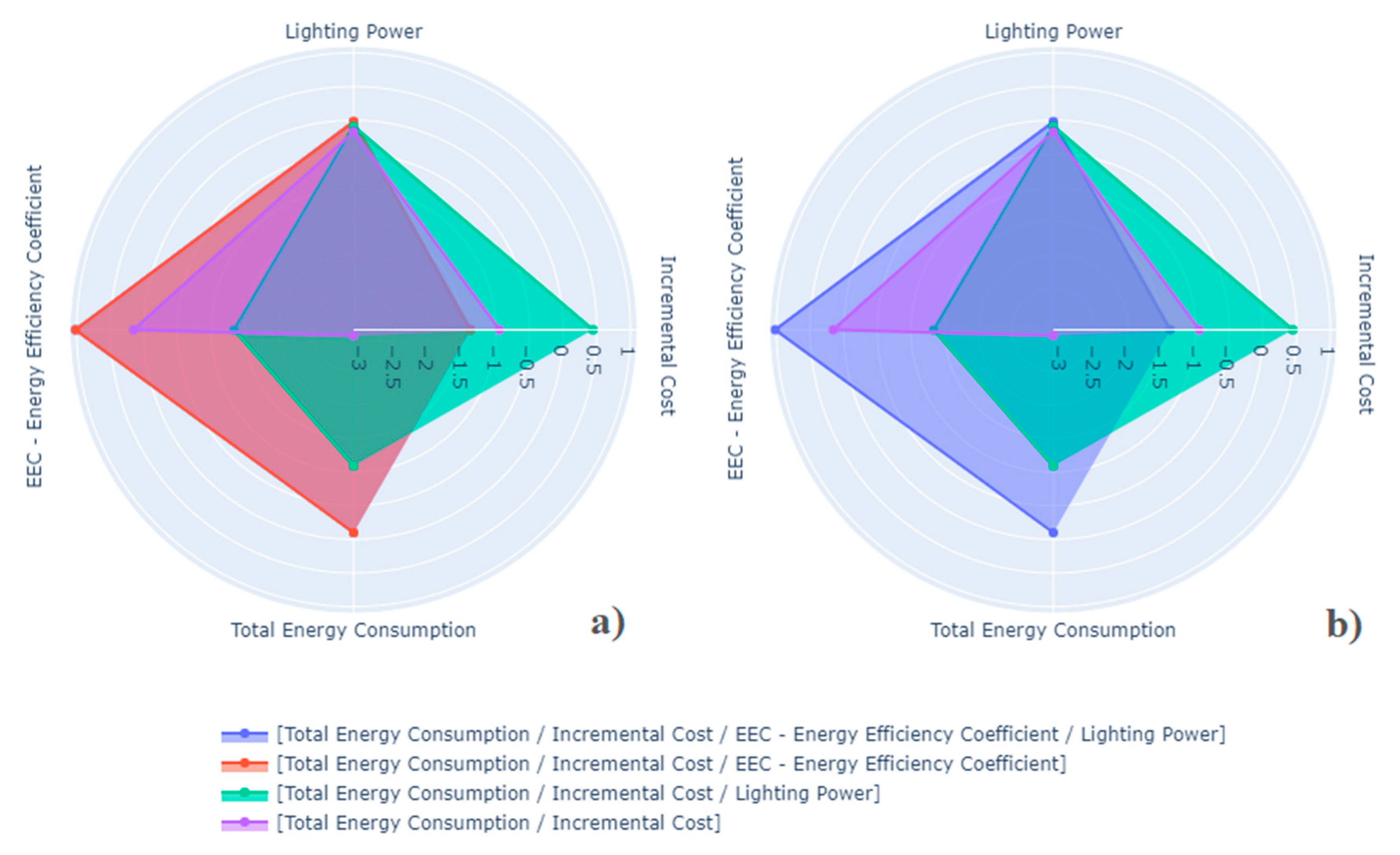
  • Case 1: Total Energy Consumption, Incremental Cost, EEC—Energy Efficiency Coefficient and Lighting Power;
  • Case 2: Total Energy Consumption, Incremental Cost and EEC—Energy Efficiency Coefficient;
  • Case 3: Total Energy Consumption, Incremental Cost and Lighting Power;
  • Case 4: Total Energy Consumption and Incremental Cost.
Knowing that data are in different scales, that is, incremental cost is given in thousands of real (Brazilian currency, R$), while the energy efficiency coefficient of the air conditioning system is between 2.0 and 5.0, it is necessary to have all in one same level to facilitate the visualization of the results. Thus, the first step in displaying these graphs is to normalize objective function data so all four objectives can be observed together in just one graph.
To observe the result of this experiment, it is important to remember that the higher the value of the Efficiency Energy Coefficient (EEC) and the lower the incremental cost, energy consumption and installed power, the better the individual. Figure 6 shows the best individual per case among 10 application tests in the proposed methodology to identify which case is the most efficient when there are “baits” in the input file.
Regarding the inference of the radar chart shown in Figure 6, the central position is the starting point and each axis represents one of the four different objectives. The performance of the best individual in each case will be evaluated in relation to all of the objectives together, regardless of the number of objective functions that make up the case. The best case will be the one with the lowest incremental cost, lowest energy consumption, lowest lighting power and highest energy efficiency coefficient possible. In other words, the best will be the polygon formed by sides closer to the central region on the axes of incremental cost (right), total energy consumption (below) and lighting power (above); and furthest from the central region on the EEC axis (left).
With the chart analysis, it can be observed that the best result when there are “baits” between the air conditioning devices was the purple diamond, representing Case 4, as it is the one that consumes the least energy among all, with reasonable values of incremental cost, lighting power and EEC. However, it is necessary to analyze the general behavior of each case in all tests performed. To help mitigate and infer these results, Table 4 was constructed.
Table 4 numerically shows the performance of all cases analyzed, divided into two parts. The first part shows the average and standard deviation of objectives and generations number needed to meet one of the stopping criteria in each case. The second part shows the total thermal capacity and lamp quantity of the best individual per case among all tests.
In Figure 6, Cases 1, 2 and 3 showed lower results than Case 4 for different reasons. The green polygon, or Case 3, does not have EEC as an objective function and, therefore, found the worst performance in that objective and higher incremental cost.
Analyzing the two views of the radar-style graph, (a) and (b), it is possible to identify that Case 1, with four objective functions, or the blue polygon is located behind the red polygon, Case 2, with three objective functions. This means that both cases found the same individual as the best by fitness in all tests accomplished. These cases presented better performance in two objectives: Incremental cost and EEC.
It is known that the less expensive the equipment, the more energy it consumes. Therefore, it is understandable that Cases 1 and 2 find a lower incremental cost, and, consequently, a higher total energy consumption. Continuing to EEC, it is important to remember two points: (1) although normalized, the EEC data are much smaller than others, and (2) the air conditioning system definitions structured in chromosome formation allow each room to have more cooling capacity than necessary defined in standards.
Analyzing the second part of the table, Cases 1 and 2 appear to be the same individual, as seen in Figure 6, since they have air conditioning capacity and identical lamp quality. Case 3 reached an individual with greater thermal capacity among the four cases, but it can be said that the variation between them is not relevant. The one that arrived at an individual with more lamps was Case 4.
In the table, an average of each Case Objective indicates their approximate value, giving an idea of the amounts that should be expected for them for algorithm users. Thereby, it can be inferred that the results were very close among themselves. The standard deviation, on the other hand, shows how dispersed the test data are compared to its objective average, denoting the variability of individuals found. The greater the standard deviation, the less “reliable” the model’s response.
To facilitate the relationship with Figure 6, the colors of the polygons were kept in the description of columns to identify each case. Another measure to collaborate to an understanding of Table 4 was the distinction between the best values of objectives and the number of generations, highlighted in gray. Thus, the highlights were Cases 2 and 4, obtaining more success in two objectives each, ratifying the behavior reproduced in the graph.
Further relating the table to the radar chart, it is observed that, despite the apparent distance observed in EEC axis of cases, the numerical variation between them is from 3.88 W/W to 4.02 W/W. Brazilian standard considers class A all devices with values above 3.24 W/W. Then, all cases found the highest rating in efficiency for the air conditioning system, even including the confidence interval, when analyzed with baits. Therefore, it can be considered that all cases found the baits and used them several times to compose the air conditioning arrangement in the base building. It is important to remember that only two baits were included.
Then, we proceeded to analyze the air conditioning system of the proposed cases. However, the authors chose not to list devices per room found in each case, showing only the quantity and percentage of use of the equipment’s baits.
The best individual selected by fitness function in all tests in Case 1 and Case 2 is the same, using the baits in 20 of 33 devices, representing 60% of the number of devices. In thermal capacity, the baits formed 84.4044 kW (288,000 BTU/h) in these cases, or 73% of the total capacity.
In Case 3, the best individual also used 20 baits, but with 36 equipment, or 52% of its air conditioning system was composed by baits. The thermal capacity of baits was 66% of the entire system, 77.3707 kW (264,000 BTU/h). Case 4 was the worst at finding the baits, forming only 35% of its air conditioning system with baits by device and 42% by thermal capacity.
Among all cases, the one that used the most baits for both quantity of devices and cooling capacity were Cases 1 and 2, with the same individual. This information, together with what was presented in Figure 6 and Table 4, reveals Case 2 as the best both by objectives values found and by the best use of baits. In view of this, the effectiveness of the proposed methodology is equally proven, finding optimal arrangements for each room formed by equipment, being in fact more efficient, employing only three objective functions.
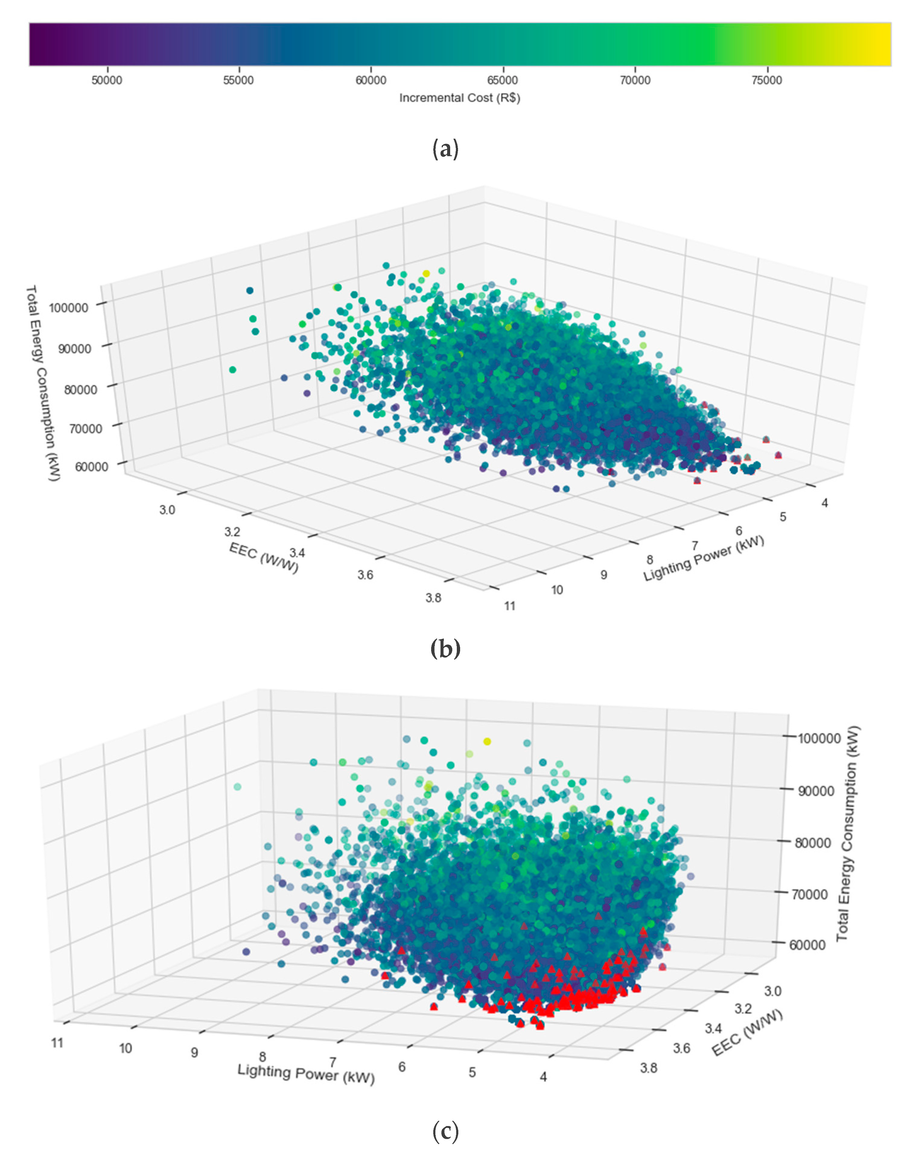
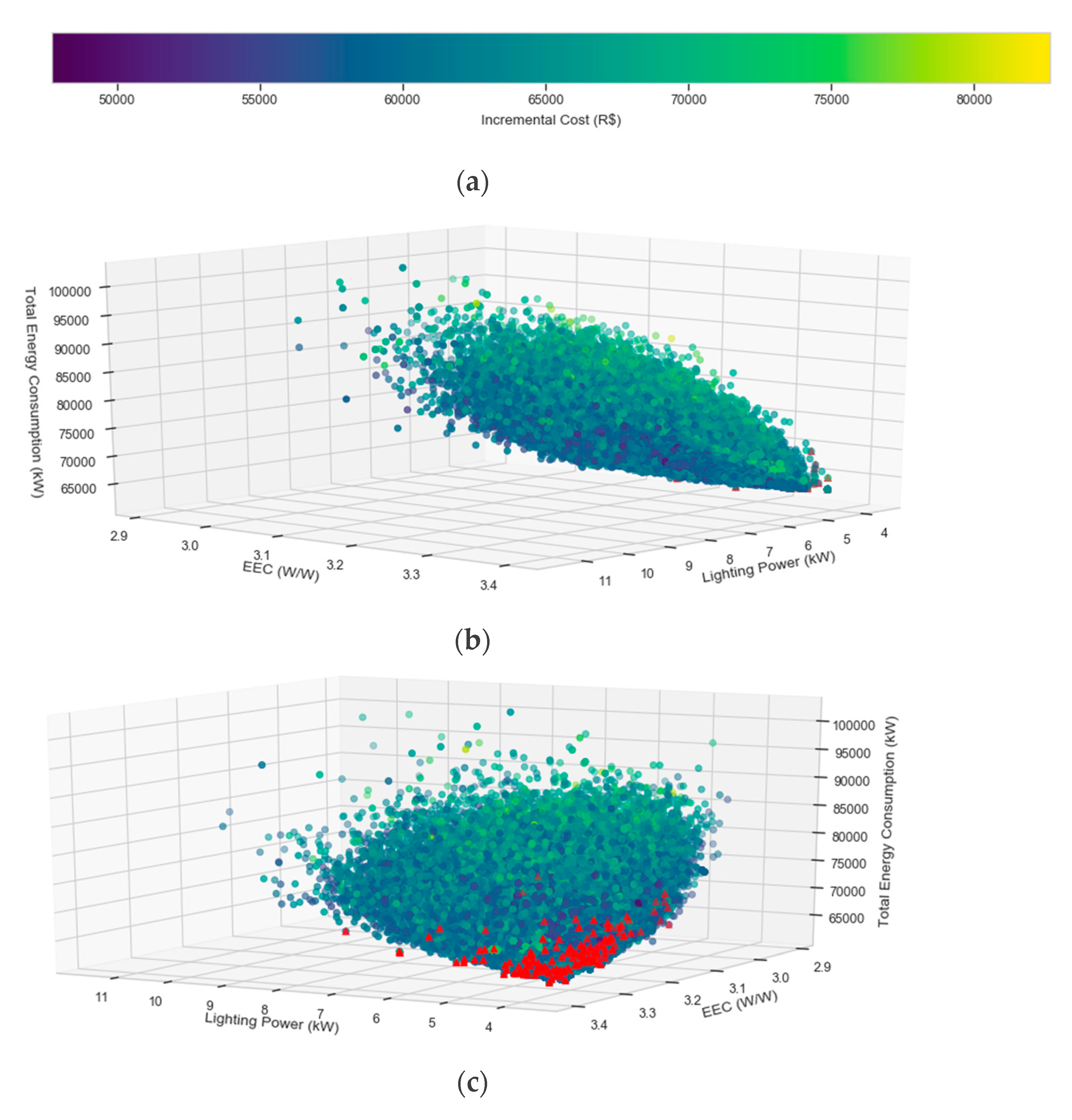
The Figure 7 shows the Pareto Curve in the form of a 3D scatterplot of the best evaluated objective function arrangement, Case 2. This graph style was chosen because it offers the possibility of presenting all four objectives at once, allowing us to plot all individuals that form the P populations of each generation of the best experiment in Case 2.
The graph axes indicate the objective functions: Total Energy Consumption (kWh), EEC (W/W) and Lighting Power (kW); and the color code shown in Figure 7a, the Incremental Cost. Yellow dots indicate the most expensive individuals, while the dark blue indicates the most affordable, or least costly, individuals. Red triangles illustrate the individuals not dominated, and there are 126 in total. It is important to mention that users can choose among these non-dominated individuals to improve their project profile, such as, for example, with lower incremental cost, or with lower consumption.
Figure 7b shows the evolution of individuals, graphically forming an arrow from generation to generation. The arrow points to the meeting point between the lowest total energy consumption, the lowest lighting power and the highest EEC. By color, a gradual darkening can be observed, starting from yellow spots, passing through green spots and, finally, arriving in spots of dark blue color. The individual’s evolution occurred as expected, improving the fitness results for each generation.
The graph third part in Figure 7c shows more adequately the non-dominated points (in red), compared to the 24,929 dominated points. There is a wide range of possibilities, principally regarding the EEC axis, which can vary from 3.0 W/W to 3.7 W/W. It is up to the user, who could be an engineer, architect or manager, to decide which point is the best for him/her.
Assigned the equipment to compose the lighting and air conditioning system by the best set of objective functions, the last step was to indicate the value of each objective for this arrangement, together with the energy cost and greenhouse gas emission data. Table 5 indicates these amounts in real, Brazilian currency, and in dollars (USD).

4.2. Validation in a Controlled Case Without “Baits”

The second phase of testing is performed to determine if the target function combination found to be the best in the experiment with adding baits will remain the best without the baits. Therefore, the same comparison studies will be made again, investigating identical conditions established in the first experiment. Likewise, 10 tests were applied for each case, keeping the previously arranged configurations and seeds fixed. The nomenclature and color codes are maintained.
As a first step, there is the normalization of the data, to arrange all the objectives on the same level to facilitate the visualization of the results. Figure 8 illustrates the best individual per case to identify which one is the most efficient without the baits previously added to the air conditioning units input file.
The inferences about the graph shown in Figure 8 are the same as those taken in Figure 6. However, there is a big difference in the results, compared to the previous experiment. This time, the better performance of Case 2, in red, is much more visible in relation to the others, at least in relation to energy consumption and lighting power. Case 2 also performed reasonably well in the other objectives. There was a considerable worsening in Case 4, in purple, considered one of the best in the bait experiment, as it found the highest total energy consumption among all. Thus, the most complete analysis is carried out using the data shown in Table 6.
Table 6 numerically shows the behavior of all cases analyzed, divided into two parts, in the same way as presented in the case with baits. As with baits, the results were very close to each other. However, it is soon apparent that in all 10 tests, Cases 1 and 2 seem to have found the same individuals because they have the same mean and standard deviation in all objectives and even in the second part of the table, referring to the best individual by fitness of each case. The instant inference is that the Illumination Power objective function is irrelevant to the problem, in view of the others. Then, between these two cases, Case 2 is chosen as the best.
Another important information recognized by Table 6 is that in all cases, the test average remained in the category A of air conditioning system efficiency, since all presented EECs were greater than 3.23 W/W, even considering the standard deviation. It is worth remembering that the table presents the data for all tests, by means and standard deviations and Figure 8, the data for the best individual per fitness for all tests. Therefore, even if Case 4 has a better average performance in the Total Energy Consumption Objective, its best individual is inferior to the best in Case 2.
Thus, the highlights in Table 6 were again Cases 2 and 4, achieving more success in two objectives each. This behavior differs from that reproduced in Figure 8, where the best was only Case 2. Therefore, Case 2 was established to compose the proposed methodology. Therefore, Figure 9 presents the Pareto Curve in a 3D scatter plot of chosen Case.
Figure 9a shows the color order of the incremental cost objective, indicating the darkest points as the least costly. Figure 9b shows the evolution of individuals, graphically forming an arrow from generation to generation. The arrow directs to the meeting point between the lowest total energy consumption, the lowest lighting power and the highest EEC, with a gradual darkening as expected and repeating the algorithm behavior when there were baits in the input file.
The third part of Figure 9c presents the non-dominated points (in red) more appropriately. Unlike the bait experiment, the range of possibilities is not as wide, especially in regards to the EEC axis, and can vary from 3.0 W/W to 3.3 W/W. That is, the non-dominated individuals are not as spread as in the bait experiment. However, it is still up to the user to choose one of the 152 non-dominated points.
Therefore, the next phase is to exhibit air conditioning and lighting system devices in Case 2, with three objective-functions: Incremental Cost, Energy Consumption and EEC. Table 7 shows a list of equipment selected to compose the analyzed systems for the base building.
It should be noted that the lighting system was essentially composed of LED lamps, the most efficient currently on the market, selecting fluorescent lamps in only one room. The most used air conditioning device was Ductless Split type. Table 8 summarize the best fitness individual from Case 2 in both experiments with and without bait.
Analyzing Table 8 with the results of both experiments, the algorithm proved to be stable and robust both in Experiment 1, with the insertion of baits in the system that most contributes to the energy cost of the building, and in Experiment 2, without the baits. Starting the investigation with the first objective, the incremental cost was practically the same in both experiments, but as for the annual energy consumption, there was a decrease of approximately 14% in the experiment without baits. This was already expected, due to the 30% increase in bait efficiency. Both experiments found greater thermal capacity than necessary established in the standards, but Experiment 1 added 10.3747 kW (35,400 BTU/h) and Experiment 2, 8.1766 kW (27,900 BTU/h). This represents a 21% reduction in this surplus from Experiment 1 to Experiment 2, affecting annual energy consumption.
Both found an EEC greater than 3.23 W/W, both rated at level A in efficiency. It is noted that the increase in efficiency in the baits raised the value of the building’s EEC by an unreal value. The energy cost and rate of greenhouse gas emissions also increased from Experiment 1 to 2, as they are proportional to energy consumption. Better representing the real situation, Experiment 2 would be responsible for the emissions of 5,144.35 tonCO2/year, at an energy cost of 8,027.34 $/year.

5. Conclusions

The importance of energy efficiency measures in buildings and their great impact on the world and national energy matrix of Brazil is undeniable. This work addressed measures on lighting and air conditioning systems and when buildings consume the most amount of energy, that is, usage of built space.
The proposed methodology is based on Brazilian regulations and standards for conscious consumption and energy efficiency in buildings. The valuation method was proposed in the guidelines of the new version of the RTQ-C, available in [5]. This methodology considers four of the main problems faced in energy efficiency studies, which are: incremental cost, total energy consumption, lighting power and air conditioning system efficiency level, which form the four candidates of objective functions of the algorithm proposed multi-objective.
From annual energy consumption, the annual rates of GHG emissions and annual energy cost were calculated. When applied to a building in use of the analyzed systems, it is also possible to find the payback from the result of the methodology in terms of energy savings and incremental cost. Likewise, it is necessary to mention that the proposed multi-objective optimization algorithm can be used in any building in hot climates that requires artificial air conditioning, as long as it is up to 35.1685 kW (120,000 BTU/h) per room.
The methodology validation occurred in a controlled case and in two stages: (1) with addition of some baits in the air conditioning input file (2 in 75 devices) and (2) without these baits. Both stages worked on the importance of using the appropriate objective function arrangement in the proposed multi-objective optimization methodology. It was analyzed case-by-case, varying objective functions proposed quantity in a pre-fixed parameter configuration. Tests for each validation step were performed 10 times, respecting equity parameters (fixed seeds).
The first stage of validation, with baits, indicated Cases 2 and 4 as the best candidates, with three and two objective functions respectively. Moving on to the selected devices arrangements by each Case verification in order to investigate which Case used more baits to compose its air conditioning system, Case 2, which considers incremental cost, total energy consumption and energy efficiency coefficient (air conditioning system), was the one that most used baits, making up 73% of building total capacity with baits. Finally, a 3D dispersion chart with color variation was displayed to indicate the population evolution in all four objectives of interest. This step served to show that the algorithm really finds the most efficient devices, as it applied the two baits in several rooms.
The second stage of validation took place to test the stability and robustness of the methodology and the optimization algorithm. The same trend was shown in the validation with baits, establishing Case 2 as the most indicated with or without baits. The results analysis and presentation were the same as in the first validation stage, including the color code and pre-fixed settings. Once the best case was chosen and configured with the best parameters for this problem, the evolution of the best individual by fitness was presented and the analyzed systems arrangements chosen. It ended with the comparison of the two experiments, quantitatively evaluating the impact of the baits on the result.
As for the algorithm usability, it is important to keep in mind that the presented methodology has great potential for the improvement and efficiency of public and private buildings organizational processes. In case of these systems retrofit, for example, the manager could include the air conditioners already in use in the input files to find out if it could be reuse in another room without losses in the building’s energy efficiency ratings according to the guidelines established in RTQ-C. Another application would be to highlight any of the four objectives, for example, the incremental cost. Thus, the chosen project would be the least costly at the time of purchase, losing a small amount in annual energy consumption, perhaps. Then, the proposed methodology would provide a variety of projects for different purposes, both in the public and private spheres.

Author Contributions

Conceptualization, S.A.M. and F.P.M.; methodology, S.A.M. and M.E.L.T.; software, F.P.M.; validation, S.A.M. and F.P.M.; formal analysis, S.A.M. and F.P.M.; investigation, S.A.M.; resources, S.A.M., F.P.M., M.E.L.T. and C.M.C.; data curation, F.P.M.; writing—original draft preparation, S.A.M.; writing—review and editing, S.A.M. and F.P.M.; visualization, M.E.L.T. and C.M.C.; supervision, M.E.L.T. and C.M.C.; project administration, S.A.M. All authors have read and agreed to the published version of the manuscript.

Funding

This research was partially funded by CAPES and CNPQ.

Acknowledgments

The authors would like to thank the entire CEAMAZON team for their technical support in energy efficiency and labeling of buildings and UFOPA Campus Oriximiná for the physical space and infrastructure.

Conflicts of Interest

The authors declare no conflict of interest.

References

  1. Lukas, S.G.; Ugursal, V.I. Modeling of end-use energy consumption in the residential sector: A review of modeling techniques. Renew. Sustain. Energy Rev. 2009, 13, 1819–1835. [Google Scholar]
  2. Santoyo-castelazo, E.; Azapagic, A. Sustainability assessment of energy systems: Integrating environmental, economic and social aspects. J. Clean. Prod. 2014, 80, 119–138. [Google Scholar] [CrossRef]
  3. Mattinen, M.K.; Heljo, J.; Vihola, J.; Kurvinen, A.; Lehtoranta, S.; Nissinen, A. Modeling and visualization of residential sector energy consumption and greenhouse gas emissions. J. Clean. Prod. 2014, 81, 70–80. [Google Scholar] [CrossRef]
  4. Balanço Energético Nacional 2019—BEN 2019. Ano Base 2018—Relatório Final; Ministério de Minas e Energia—MME, Empresa de Pesquisa Energética—EPE: Rio de Janeiro, Brazil, 2019.
  5. CB3E, Centro Brasileiro de Eficiência Energética em Edificações: 2017. Proposed Method for the Evaluation of Energy Efficiency Based on Primary Energy in Commercial, Service and Public Buildings (Version 3); Department of Civil Engineering, Federal University of Santa Catarina: Florianopolis, Brazil, 2017. [Google Scholar]
  6. Perera, A.T.D.; Sirimanna, M.P.G. A Novel Simulation Based Evolutionary Algorithm to Optimize Building Envelope for Energy Efficient Buildings. In Proceedings of the 7th International Conference on Information and Automation for Sustainability, Colombo, Sri Lanka, 22–24 December 2014. [Google Scholar]
  7. Bingham, R.; Agelin-Chaab, M.; Rosen, M.A. Multi-objective Optimization of a Residential Building Envelope in the Bahamas. In Proceedings of the 5th IEEE International Conference on Smart Energy Grid Engineering, Oshawa, ON, Canada, 14–17 August 2017. [Google Scholar]
  8. Harun, M.F.; Samah, A.A.; Majid, H.A.; Yusoff, Y.; Lim, Y.W. Optimization of Green Building Design to Achieve Green Building Index (GBI) Using Genetic Algorithm (GA). In Proceedings of the 6th ICT International Student Project Conference, Skudai, Malaysia, 23–24 May 2017. [Google Scholar]
  9. Yan, C.W.; Yao, J. Research on the Optimization of Building Energy Efficient Measures Based on Incremental Costs. In Proceedings of the 2nd International Conference on Computer Engineering and Technology, Chengdu, China, 16–18 April 2010. [Google Scholar]
  10. Liu, J.; Yu, X.; Qi, B. Building materials’ optimization based on fuzzy pattern-recognition. In Proceedings of the International Conference on Management and Service Science, Wuhan, China, 20–22 September 2009. [Google Scholar]
  11. Chandrasekara, P.D.M.; Chathurangi, W.L.D.M.; Kodikara, I.N.; Kumara, N.C.T. Agent based Building Automation and Control System for moderate scale buildings. In Proceedings of the International Conference on Electrical, Electronics, and Optimization Techniques, Chennai, India, 3–5 March 2016. [Google Scholar]
  12. Oezluek, A.C.; Ploennigs, J.; Kabitzsch, K. A Generic Framework for Synthesis and Optimization of System Designs in the Example of Building Automation Systems. In Proceedings of the IEEE 15th Conference on Emerging Technologies & Factory Automation, Bilbao, Spain, 13–16 September 2010. [Google Scholar]
  13. Fanti, M.P.; Mangini, A.M.; Roccotelli, M.; Iannone, F.; Rinaldi, A. A Natural Ventilation Control in Buildings Based on Co-Simulation Architecture and Particle Swarm Optimization. In Proceedings of the IEEE International Conference on Systems, Man, and Cybernetics, Budapest, Hungary, 9–12 October 2016. [Google Scholar]
  14. Martirano, L.; Manganelli, M.; Parise, L.; Sbordone, D.A. Design of a fuzzy-based control system for energy saving and users comfort. In Proceedings of the 14th International Conference on Environment and Electrical Engineering, Krakow, Poland, 10–12 May 2014. [Google Scholar]
  15. Liu, X.F.; Liu, J.P.; Lui, L.; Zou, W. The Design and Application of the Optimize Control Management System to the Central Air-Conditioning Based on Intelligent Building Technology. In Proceedings of the International Conference on Electric Technology and Civil Engineering (ICETCE), Lushan, China, 22–24 April 2011. [Google Scholar]
  16. Fan, R.; Li, Y.; Cao, Y.; Xie, W.; Tan, Y.; Cai, Y. An Optimization Management Strategy for Energy Efficiency of Air Conditioning Loads in Smart Building. In Proceedings of the IEEE 16th International Conference on Environment and Electrical Engineering, Florence, Italy, 7–10 June 2016. [Google Scholar]
  17. Zhou, W.; Yan, J.W.; Lin, H.J. The Energy Efficiency Monitoring and Operation Optimization of Central Air Conditioners. In Proceedings of the 26th Chinese Control and Decision Conference, Changsha, China, 31 May–2 June 2014. [Google Scholar]
  18. Javed, A.; Larijani, H.; Ahmadinia, A.; Emmanuel, R. Modelling and optimization of residential heating system using Random Neural Networks. In Proceedings of the IEEE International Conference on Control Science and Systems Engineering, Yantai, China, 29–30 December 2014. [Google Scholar]
  19. Si, W.; Ogai, H.; Hirai, K.; Takahashi, H.; Ogawa, M. An Improved PSO Method for Energy Saving System of Office Lighting. In Proceedings of the SICE Annual Conference, Tokyo, Japan, 13–18 September 2011. [Google Scholar]
  20. Zhang, D.; Xia, X. Distributed illumination control of LED networked systems via local occupancy information. In Proceedings of the IEEE 56th Annual Conference on Decision and Control, Melbourne, Australia, 12–15 December 2017. [Google Scholar]
  21. Choeychuen, K. Fuzzy membership function optimization for smart LED lamp using particle swarm optimization. In Proceedings of the International Workshop on Advanced Image Technology, Chiang Mai, Thailand, 7–9 January 2018. [Google Scholar]
  22. Altayeva, A.; Omarov, B.; Cho, Y.I. Multi-Objective Optimization for Smart Building Energy and Comfort Management as a Case Study of Smart City Platform. In Proceedings of the IEEE 3rd International Conference on Data Science and Systems, Bangkok, Thailand, 18–20 December 2017. [Google Scholar]
  23. Wang, F.; Zhou, L.; Ren, H.; Liu, X.; Shafie-khah, M.; Catalão, J.P.S. Multi-objective Optimization Model of Source-Load-Storage Synergetic Dispatch for Building Energy System Based on TOU Price Demand Response. In Proceedings of the IEEE Industry Applications Society Annual Meeting, Cincinnati, OH, USA, 1–5 October 2017. [Google Scholar]
  24. Godina, R.; Rodrigues, E.M.G.; Pouresmaeil, E.; Matias, J.C.O.; Catalão, J.P.S. Model Predictive Control Technique for Energy Optimization in Residential Sector. In Proceedings of the IEEE 16th International Conference on Environment and Electrical Engineering, Florence, Italy, 7–10 June 2016. [Google Scholar]
  25. Report: Factors for Converting Electrical and Thermal Energy into Primary Energy and Carbon Dioxide Emissions to be Used in the Labeling of Energy Efficiency Levels in Buildings (Version 1); Technical Report; Electric Energy Brazilian Agency (ANEEL): Brasilia, Brazil, 2016.
  26. CELPA. Available online: http://www.celpa.com.br/residencial/informacoes/cobranca-de-tarifas (accessed on 31 March 2020).
  27. Asare-bediako, B.; Ribeiro, P.F.; Kling, W.L. Integrated energy optimization with smart home energy management systems. In Proceedings of the 3rd IEEE PES Innovative Smart Grid Technologies Europe, Berlim, Germany, 14–17 October 2012. [Google Scholar]
  28. Anflor, C.T.M. Otimização Evolucionária e Topológica em Problemas Governados pela Equação de Poisson Empregando o Método dos Elementos de Contorno. Ph.D. Thesis, Federal University of Rio Grande do Sul, Porto Alegre, Brazil, 2007. [Google Scholar]
  29. Zitzler, E.; Thiele, L. An Evolutionary Algorithm for Multi-objective Optimization: The Strength Pareto Approach—Technical Report 43. In Computer Engineering and Communication Networks Lab (TIK); Swiss Federal Institute of Technology (ETH): Zurich, Switzerland, 1998. [Google Scholar]
  30. Ghararia, R.; Poursalehib, N.; Abbasib, M.; Aghaieb, M. Implementation of Strength Pareto Evolutionary Algorithm II in the Multi-objective Burnable Poison Placement Optimization of KWU Pressurized Water Reactor. Nuclear Eng. Technol. 2016, 48, 1126–1139. [Google Scholar] [CrossRef] [Green Version]
  31. Zhao, F.; Lei, W.; Ma, W.; Liu, Y.; Zhang, C. An Improved SPEA2 Algorithm with Adaptive Selection of Evolutionary Operators Scheme for Multi-objective Optimization Problems. Math. Probl. Eng. 2016, 2016, 8010346. [Google Scholar] [CrossRef] [Green Version]
  32. Lesinski, G. Application of the Strength Pareto Evolutionary Algorithm (SPEA2) Approach to Rail Repair Investments; C/NRCD Internal Research and Development Project, Technical Report; United States Military Academy: New York, NY, USA, 2016. [Google Scholar]
  33. Alves, D.N.; Saúde, R.R.C. Procedimento Básico de Elaboração e Implantação de Projetos de Sistemas de Ar Condicionado Baseado na ABNT NBR 16401. Bachelor’s Thesis, Federal University of Espirito Santo, Vitória, Brazil, 2013. [Google Scholar]
  34. Roriz, M. Uma Proposta de Revisão do Zoneamento Bioclimático Brasileiro; ANTAC National Association of Built Environment Technology: Sao Paulo, Brazil, 2012. [Google Scholar]
Figure 1. Brazilian matrix of electricity consumption by sector—BEN 2019 [4].
Energies 13 03303 g001
Figure 2. Proposed methodology for the optimization multi-objective of buildings air conditioning and lighting systems.
Energies 13 03303 g002
Figure 3. Chromosome developed to address the problem.
Energies 13 03303 g003
Figure 4. Chromosome formation process of the proposed methodology flowchart.
Energies 13 03303 g004
Figure 5. Model building rooms and floors layout, with number of users per room and dimensions.
Energies 13 03303 g005
Figure 6. Best individual among all tests performed per case with “baits” (a) showing all 4 cases together and (b) without Case 2, the red.
Energies 13 03303 g006
Figure 7. Pareto Curve in the form of a 3D scatterplot (a) The color scale of the Incremental Cost Objective, (b) Pareto Curve of Case 2—With Lures and (c) Pareto Curve of Case 2—With Lures turned at approximately 270°.
Energies 13 03303 g007
Figure 8. Best individual among all tests performed per case without baits (a) showing all 4 cases together and (b) without Case 2, the red.
Energies 13 03303 g008
Figure 9. Pareto Curve in the form of a 3D scatterplot (a) The color scale of the Incremental Cost Objective, (b) Pareto Curve of Case 2—Without Baits and (c) Pareto Curve of Case 2—Without Baits turned at approximately 270°.
Energies 13 03303 g009
Table 1. Required data in each input file of the proposed methodology.
Air ConditioningRoom; Range; Quantity; Type; Capacity (BTU/h); Power (W); Price (R$)
LightingRoom; Luminaire/Room; Lamps/Luminaire; Lamps Total; Type; Power (W); Luminous flux; Price (R$)
ActivitiesIndex; Building Function; DPL Class A (W/m2); DPL Class B (W/m2); DPL Class C (W/m2); DPL Class D (W/m2); Desired illuminance (LUX)
BuildingActivity 1; Activity 2; Activity 3; Electricity Price; Utilization (h/d); Utilization (d/y); Length; Width; floor/ceiling height; Number of Floors; Wall Thickness; Geographical orientation of the main facade; Aperture 1, 2, 3 and 4 (%); Window: External protection;
Window: Internal Protection; Common Glass; Slab ceiling;
RoomsIndex; Floor; Side; Function; Number of Users; Width; Length; Area.
Table 2. Cooling capacity value ranges defined in the methodology.
RangeCooling Capacity (kW)Cooling Capacity (BTU/h)
11.4653 kW to 2.3445 kW 5000 to 8000 BTU/h
22.4911 kW to 3.3703 kW8500 to 11,500 BTU/h
33.5168 kW to 4.3960 kW12,000 to 15,000 BTU/h
44.6891 kW to 6.1544 kW16,000 to 21,000 BTU/h
56.4475 kW to 7.6198 kW22,000 to 26,000 BTU/h
67.9129 kW to 9.3782 kW27,000 to 32,000 BTU/h
79.6713 kW to 10.5505 kW33,000 to 36,000 BTU/h
811.1367 kW to 12.3089 kW38,000 to 42,000 BTU/h
912.6020 kW to 14.0674 kW43,000 to 48,000 BTU/h
1014.9466 kW to 15.8258 kW51,000 to 54,000 BTU/h
1116.1189 kW to 17.5842 kW55,000 to 60,000 BTU/h
Table 3. “Baits” equipment included in the “Air conditioning” input file.
IndexTypeCooling Capacity (kW)Cooling Capacity (BTU/h)RangeElectric Power (W)CEE (W/W)Price (R$)
23Window3.51612,00037734.551482.90
64Ceiling-Suspended10.55036,000723204.552799.30
Table 4. Evaluation of the results obtained in the experiments to analyze the best case for the fitness function formation of proposed methodology—With Baits.
Objective FunctionCase 1Case 2Case 3Case 4
Total Energy Consumption54,955.82 ± (1196.12)54,518.35 ± (481.82)56,110.74 ± (544.53)54,915.84 ± (694.27)
Incremental Cost56,433.48 ± (2641.31)57,378.26 ± (3107.55)55,617.34 ± (2158.74)55,776.44 ± (883.08)
Energy Efficiency Coefficient3.99 ± (0.10)4.02 ± (0.06)3.88 ± (0.08)4.00 ± (0.07)
Lighting Power4.13 ± (0.09)4.13 ± (0.09)4.11 ± (0.11)4.01 ± (0.17)
Generations Numbers3662.60 ± (1055.74)3776.60 ± (860.28)2502.75 ± (682.48)3,882.60 ± (1096.19)
Total Cooling Capacity (BTU/h)393,000.0393,000.0397,000.0392,000.0
Total Cooling Capacity (kW) 115.1769115.1769116.3492114.8838
Number of Lamps253253257275
Table 5. Summary of the best fitness individual from Experiment 1—With Baits.
Experiment 1Model Value
Incremental Cost (R$)60,850.40
Incremental Cost ($)11,561.57
Total Energy Consumption (kWh/year)54,171.6
Energy Consumption – Lighting (kWh/year)6941.76
Energy Consumption—Air Conditioning (kWh/year)47,229.84
Thermal Capacity393,000
CEE Total (W/W)3.94
Energy Efficiency Level (RTQ-C)—Air Conditioning SystemA
Power—Lighting (kW)4.13
Energy Efficiency Level (RTQ-C)—Lighting SystemA
Energy Cost (R$/year)36,348.06
Energy Cost ($/year)6906.13
GHG Emissions (ton CO2/year)4425.81
Table 6. Evaluation of the results obtained in the experiments to analyze the best case for the fitness function formation of proposed methodology—Without Baits.
Objective FunctionCase 1Case 2Case 3Case 4
Total Energy Consumption62,959.01 ± (539.80)62,959.01 ± (539.80)65,640.96 ± (6088.02)62,729.52 ± (747.53)
Incremental Cost62,229.93 ± (2272.17)62,229.93 ± (2272.17)62,764.59 ± (1849.94)65,125.05 ± (3599.16)
Energy Efficiency Coefficient3.34 ± (0.04)3.34 ± (0.04)3.32 ± (0.07)3.37 ± (0.02)
Lighting Power3.97 ± (0.19)3.97 ± (0.19)4.15 ± (0.39)4.08 ± (0.10)
Generations Numbers2246.20 ± (674.09)2246.20 ± (674.09)2620.80 ± (1350.39)2721.40 ± (901.83)
Cooling Capacity
(BTU/h)
383,500.0383,500.0441,000.0386,000.0
Cooling Capacity
(kW)
112.3927112.3927129.2443113.1254
Number of Lamps253253257275
Table 7. Devices selected by the algorithm.
Lighting System
RoomLuminaireLamps
IndexLamps/LumLum/RoomTypeLuminous FluxPower (W)Price (R$)
1181LED Compact9771110.05
2101LED Tube17442020.00
352LED Tube17442020.00
4151LED Tube17442020.00
593LED Compact9771111.00
6161LED Tube10961535.00
763LED Compact9771110.05
8151LED Tube11791529.00
9151LED Tube11791529.00
1062Compact Fluorescent1500235.90
1163LED Compact9771111.00
12271LED Compact9771111.00
13191LED Tube14322035.00
14271LED Compact9771110.05
15271LED Compact9771111.00
Air Conditioning System
RoomRangeQuantityTypeCooling Capacity in kW (and BTU/h)Cooling Capacity /Room in kW (and BTU/h)Power (W)Price (R$)
113Ductless Split2.6376 (9000)7.9129 (27,000)7191965
201Ductless Split2.1980 (7500)5.7148 (19,500)6911035
221Ductless Split3.5168 (12,000)10681799
322Ductless Split3.5168 (12,000)7.0337 (24,000)10101291
441Ductless Split6.4475 (22,000)9.6713 (33,000)19891792
411Ceiling Cassette3.2237 (11,000)9961300
514Ductless Split2.6376 (9000)10.5505 (36,000)7191965
603Ductless Split2.1980 (7500)6.5940 (22,500)6911299
721Ductless Split3.5168 (12,000)5.7148 (19,500)10961499
701Ductless Split2.1980 (7500)6911299
822Ductless Split3.5168 (12,000)7.0337 (24,000)10101291
913Ductless Split2.6376 (9000)7.9129 (27,000)7191965
1001Ductless Split2.1980 (7500)4.3960 (15,000)6781796
1001Window2.1980 (7500)754938
1122Ductless Split3.5168 (12,000)7.0337 (24,000)10751320
1231Ductless Split5.2752 (18,000)8.7921 (30,000)16002545
1221Ductless Split3.5168 (12,000)10101291
1351Ductless Split8.7921 (30,000)8.7921 (30,000)26903509
1451Ductless Split8.2059 (28,000)8.2059 (28,000)27003000
1522Ductless Split3.8099 (13,000)7.6198 (26,000)11181500
Table 8. Summary of the best fitness individual from Case 2 to Experiment 1 and 2—No Bait.
Quantities AnalyzedExperiment 1Experiment 2
Incremental Cost (R$)60,850.4060,741.95
Incremental Cost ($)11,561.5711,540.97
Total Energy Consumption (kWh/year)54,171.662,966.40
Energy Consumption—Lighting (kWh/year)6941.766431.04
Energy Consumption—Air Conditioning (kWh/year)47,229.8456,535.36
Cooling Capacity (BTU/h)393,000385,500
Cooling Capacity (kW)115.1769112.9788
CEE Total (W/W)3.943.31
Energy Efficiency Level (RTQ-C)—Air Conditioning SystemAA
Power—Lighting (kW)4.133.82
Energy Efficiency Level (RTQ-C)—Lighting SystemAA
Energy Cost (R$/year)36,348.0642,249.19
Energy Cost ($/year)6906.138027.34
GHG Emissions (ton CO2/year)4425.815144.35

