An Energy Model Using Sleeping Algorithms for Wireless Sensor Networks under Proactive and Reactive Protocols: A Performance Evaluation

Abstract

The continuous evolution of the Internet of Things (IoT) makes it possible to connect everyday objects to networks in order to monitor physical and environmental conditions, which is made possible due to wireless sensor networks (WSN) that enable the transfer of data. However, it has also brought about many challenges that need to be addressed, such as excess energy consumption. Accordingly, this paper presents and analyzes wireless network energy models using five different communication protocols: Ad Hoc On-Demand Distance Vector (AODV), Multi-Parent Hierarchical (MPH), Dynamic Source Routing (DSR), Low Energy Adaptive Clustering Hierarchy (LEACH) and Zigbee Tree Routing (ZTR). First, a series of metrics are defined to establish a comparison and determine which protocol exhibits the best energy consumption performance. Then, simulations are performed and the results are compared with real scenarios. The energy analysis is conducted with three proposed sleeping algorithms: Modified Sleeping Crown (MSC), Timer Sleeping Algorithm (TSA), and Local Energy Information (LEI). Thereafter, the proposed algorithms are compared by virtue of two widely used wireless technologies, namely Zigbee and WiFi. Indeed, the results suggest that Zigbee has a better energy performance than WiFi, but less redundancy in the topology links, and this study favors the analysis with the simulation of protocols with different nature. The tested scenario is implemented into a university campus to show a real network running.

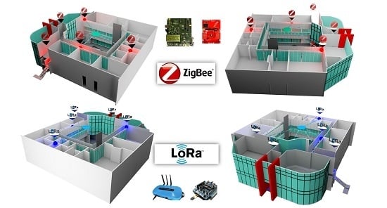
1. Introduction

Humanity is continuously changing and adapting technology to satisfy their hobbies, wishes, and necessities. Accordingly, wireless technologies evolve over time, becoming more user-friendly and convenient with each passing year. The interconnection of electronic devices is one such technology, which is made possible due to the creation of protocols with different network topologies. A network topology is a set of devices that are interconnected through communication links. Indeed, the generality of this definition has allowed the development of different models to represent different types of topologies. Sensors play a crucial role in the automation processes as they provide information on the environment and physical quantities [1]. Consequently, it is vital to ensure that they provide accurate measurements since the collected data is used for decision-making. Wireless sensor networks (WSNs) are based on different sensing nodes capable of obtaining information from the environment, processing these data locally, and communicating with a central coordinator node or base station via wireless links [2].

Currently, the main objective in the WSNs is to study the behavior concerning the energy consumption of the wireless technologies under different perspectives of routing protocols. To achieve this, multiple strategies must be designed to compare their consumption. Then, knowing these strategies will allow determining which ones are most suitable for each occasion. Since, the size and battery characteristics make power consumption a critical factor in its design.

From the need to optimize energy consumption, new research topics appear, such as energy collection and consumption optimization [3,4].

The strategies for energy management in WSNs may be classified in schemes and protocols for improving the energy provision or energy consumption [5]. The first group includes schemes for battery-driven systems, with energy harvesting and transference, the second group is related to schemes for systems data-driven, duty cycling of the WSNs nodes and mobility-based energy conservation [5]. Other classification of the WSNs energy management strategies takes into account the application; in [6] there is a detailed classification of the strategies of energy harvesting in WSNs related to transmission policy (fixed or variable transmission power and probability distribution), energy balancing, duty cycling. In [7] there is a comparison of maximum power density possible for WSNs from each kind of energy harvesting technologies (solar, vibrational, electromagnetic, wind, ambient RF energy) and an evaluation of the performance of the possible design alternatives. Recent works [8] have compared the energy management in WSNs algorithms based on intelligent machine-learning, which is considered the emerging trend and future direction of the research [9].

Home networks or smart grids allow the integration of renewable energies, limit consumption peaks, and improve energy efficiency [10,11]. Improving energy efficiency will make it possible to use energy harvesting or energy scavenging techniques [12,13], which can provide new energy to the nodes. These techniques extract energy from the medium, for example, from solar radiation, wind, temperature differences, movement, and so on. These techniques generally provide relatively low amounts of energy, and many of them are not constant, but these drawbacks may be overcome if the energy requirements are less than the average energy generated.

Therefore, the less energy a sensor node consumes, it will be able to work longer for the same stored energy. Besides, if energy requirements are low, the spectrum of energy harvesting techniques that could be used will be broader. One of the most widely used energy sources is solar. This is because both the energy source and the technology are prevalent, and very high yields are obtained compared to other sources. For example, in [12], a follower of the maximum power point of solar panels applied to sensor network nodes is proposed to obtain the maximum energy with which to recharge a battery. Another source that has been widely applied is piezoelectric, where energy is extracted from the movements or vibrations. For example, in [14], some cells of piezoelectric material are used to take advantage of the water currents in seas and rivers to generate a few milliwatts, but enough to charge a battery. Other techniques [15] that use the advantages of programming and algorithms are routing protocol rules-based mechanisms and sleeping node techniques.

Among the features that impact the deployment of WSNs are wireless technologies and routing protocols. There are studies on WiFi and ZigBee technologies to determine which of them would have a lower energy impact on smart power grids [16]. Therefore, it is important to define the most appropriate technology from all points of view, including the energy consumption of the devices that make up these smart grids. Then, it is relevant to define the most used technologies from different points of view, including the energy consumption of the devices that constitute the said smart grids, such as WiFi and Zigbee.

Zigbee is a wireless communications standard designed by Zigbee Alliance. Indeed, devices based on Zigbee technology are cheap, and their ability to generate networks with mesh topology results in significant energy reduction [17]. In essence, Zigbee is a standardized set of solutions that can be implemented by any manufacturer. The medium access control (MAC) layer is based on the IEEE 802.15.4 standard of the personal area wireless networks and targets applications that need secure data communications with low transmission rates as well as at maximizing the battery life. For industrial, scientific, and medical uses, Zigbee uses the ISM band, specifically 868 MHz in Europe, 915 MHz in the United States, and 2.4 GHz worldwide, which is a band typical of WiFi. For simplicity, the most common is that Zigbee device manufacturers opt for this band, which guarantees that the smart device can work anywhere. On the other hand, it is easier for this band to saturate if we increase the number of devices operating in the same band. Indeed, the importance that these intelligent energy networks will have in the future is currently forcing companies to seek appropriate technologies.

Furthermore, the choice of communications technology is critical, given the dimension that these energy networks will acquire in the near future [18]. Mesh networks offer advantages in energy saving and offer significant security in data transmission since they allow multipath routes to be established, with alternative routes available in the case that nodes are blocked or out of service. This is one of the characteristics of Zigbee technology that the WiFi networks have attempted to assimilate. WiFi networks operate without a license in the 2.4 GHz and 5 GHz radio bands, with data transmission rates of 11 Mbps (802.11b) or 54 Mbps (802.11a) or by employing some products that support both bands (dual band). Indeed, they have similar performance to wired 10BaseT or Ethernet networks [19]. The topology reconfiguration is conducted by the routing protocols that are responsible for directing the packets and optimizing the node functions so that they belong to the network; moreover, the said protocols also ensure that the nodes send and receive and packets and that they are constantly listening to the communication channels. Indeed, these protocols seek to optimize the energy consumption of wireless networks according to size and the number of devices.

For instance, sleeping techniques are available wherein nodes fall asleep if they do not have immediate tasks in the network [20], the main advantages of which are low energy consumption and easy integration through the nodes. Herein, each sensor only needs to be turned on when data needs to be sent to another device, whereas routers and coordinators must be turned on every time. Data transmission occurs in three ways: continuously in the fixed intervals [21], directed by events, and directed by query. Hybrid systems also exist that use a combination of data transmission techniques, such as economizing communication distance.

Sensor networks use energy-aware protocols to optimize battery life. These protocols are based on the fact that using the path of least resistance is not always the best solution from the point of view of increasing network life and connectivity [22]. An example of this type of protocol that is widely used in the existing literature is the low energy adaptive clustering hierarchy (LEACH) [23], which is a cluster-based protocol that includes distributed cluster information. LEACH randomly selects some nodes and considers them as master nodes, the goal is to be able to distribute the energy evenly over the entire network. In this work, multiple scenarios of WSNs are proposed under different routing protocols, the objective of which is to investigate the performance of each WSN based on three widely known protocols: Ad hoc On-demand Distance Vector (AODV) [24], Dynamic Source Routing (DSR) [25], and Multi-Parent Hierarchical (MPH) [26]. To compare these protocols, performance metrics are defined for each, and simulations are run accordingly, the results of which are analyzed to obtain the optimal protocols. Two real scenarios are then implemented in order to compare energy performance with the said simulations. Finally, energy analysis is conducted using two proposed sleeping algorithms: Modified Sleeping Crown (MSC) algorithm and Timer Sleeping Algorithm (TSA).

The motivation of this work is to analyze the impact of performance metrics that directly influence the energy consumption of the sensors. The novelty of the proposal consists of the implementation in a real scenario of Zigbee and WiFi networks under different nature routing protocols (proactive, reactive, hybrid, and energy-aware). Furthermore, this work proposes three sleeping techniques to optimize the energy of the nodes, two of which are algorithm proposals by the authors themselves.

The structure of the manuscript is as follows: Section 2 describes Materials and Methods with a general classification of the sleeping techniques in the WSNs. Section 3 consists of the experimental results related to the performance metrics employed to compare the routing protocols as well as the simulation parameters with the real tests. Section 4 describes the discussion and compares them with the simulations; it uses these comparisons to extrapolate nodes with respect to the proposed algorithms. Finally, the conclusions are given in Section 5.

2. Materials and Methods

The routing algorithms in WSNs are responsible for monitoring the delivery of information as well as for meeting the following standards: to maintain a routing table easy to handle and with the least possible number of obsolete routes; to choose the best route for a given destination, either the fastest, most reliable, best capacity, or minimal cost route; to maintain the table of neighbors or routing for possible reconfigurations of the topology (connections and disconnections of nodes), and finally to require a small number of messages and time to converge (low overhead) [27].

Currently, the literature divides the topologies of sensor networks into two categories: hierarchical networks and mesh networks. The debate is centered around which is the better network and which presents greater benefits. Obviously, both topologies are useful and valid in their own right, and each has its own advantages according to different performance metrics, such as distance, network density, interoperability, and mobility. Thus, in a network where a router node fails, a mesh topology can end up in the form of a star. This means that resilience is also a parameter that plays a fundamental role in analyzing the ideal functioning of a protocol. Resilience is the ability of a node or a network to overcome changes that may occur. For example, a network may be prone to some changes in link configuration and topology due to the interference or node connections and disconnections. The time it takes for the network to reconfigure its links and thus return to a stable state can be measured as the resilience parameter. In addition, it is also necessary to take into account the number of coordinating nodes as well as their spatial distribution in the network. This work has a coordinating node, which is the only destination of information; in other words, it is a single point of failure. However, in this application, the reaction of the routing protocol against the topology configuration and the formation of node links is shown.

The most popular hierarchical WSN protocols consist of the following: SHRP (Simple Hierarchical Routing Protocol) [28], LEACH (Low Energy Adaptive Cluster Hierarchy) [29], PEGASIS (Power-Efficient Gathering in Sensor Information System) [30], HEAP (Hierarchical Energy-Aware Protocol for routing and Aggregation in Sensor networks) [31], HPEQ (Hierarchical Periodic, Event-driven and Query-based) [32], among others. This paper emphasizes some characteristic protocols in order to compare their energy performance, actually determined in real Zigbee and WiFi networks, as well as the proposed sleeping techniques. In the LEACH protocol, there are two phases of operation: cluster formation and stable status. Cluster formation uses a random access protocol where the nodes choose themselves as cluster heads depending on whether they have previously taken this role. Once the clusters have been formed, the nodes transmit their information using a time-division multiple access structure without collisions.

Besides, the sensor network protocols may be further divided into two groups: namely proactive and reactive protocols. In reactive protocols, the nodes require a path only if it is required. This determines a high latency for the first data packet. On the other hand, in the proactive protocols, the sensor nodes always have information about all nodes of the whole network. Some of these protocols are explained below.

The AODV routing protocol, a reactive protocol, is based on the efficiency of routing for ad hoc WSNs that have a large number of nodes, using a route discovery mechanism in the broadcast mode. Indeed, AODV is able to transmit in either the unicast or multicast mode. In addition, it uses the bandwidth in an efficient way and also responds rapidly to the changes of the network, thereby preventing any network loops [24]. Alternatively, DSR protocol has some advantages. For instance, a node can get multiple paths toward a specific destination by requiring a path. Besides, it allows the network to be fully self-configuring, without the necessity of a specific architecture or topology. Furthermore, DSR is useful when a node moves continuously, since it adapts quickly to the routing changes; it also leads to a decrease of the overhead in the network [33].

Additionally, the Zigbee tree routing (ZTR) is a simple protocol that defines some parent-child-type links with the child nodes, thus bringing the information to their parent nodes. In turn, parent nodes give network access to the child nodes, thereby creating parent-child links. Zigbee technology requires that there be at least one device with full functionality acting as a sink coordinator, but end devices have reduced functions in order to reduce costs. Indeed, ZTR is advantageous insofar that for the algorithm implemented at the network layer, there is a good balance between the unit cost, battery expense, and complexity of its implementation, to thereby obtain a proper cost-performance ratio for the specific application [34].

Finally, in the MPH protocol, a network with a hierarchical structure is created where the hierarchy of the employed nodes is determined by their location; in other words, it uses proactive protocols. In essence, this functions like a hierarchical tree: the nodes decide the parent and child links, so as to determine the possible paths. The connections between the parent and child nodes are defined according to the coverage radius, which in turn is a function of the transmitted power. Consequently, each node shares children and parent nodes with any other node, obviously belonging to the same level of the hierarchical structure, which allows more links but does not generate unnecessary routes. This protocol benefits from the controlled maintenance of defined paths resulting from its proactive nature but matches the agility that allows having more than one path for each node. This feature makes it particularly versatile and suitable for different applications and topologies [26].

The best way to save energy is to implement sleeping techniques, allowing sensor nodes to change to low power consumption modes, thereby saving energy when the primary tasks are not being performed. The sleeping techniques can be grouped into two main typologies: medium access control (MAC) sleeping techniques and routing layer techniques [35].

2.1. MAC Sleeping Techniques

The MAC layer allows the sensor nodes to efficiently access the medium in question. Moreover, multiple protocols implement sleep techniques in this layer. These techniques can be classified into two categories [35,36]. These are outlined below.

• Synchronous: the nodes are synchronized, i.e., when wake-up is scheduled, the sleeping nodes wake-up at the same time. When the nodes are active, a MAC approach can be used. However, the main disadvantage of this technique is the need for control messages to synchronize the node times. As an example, we refer to some works based on the sleep/wake schedule, as cited in [37]. The authors focus on a used synchronization scheme and show that its synchronization error is non-negligible, and using a conservative time is energy wasteful [38].
• Asynchronous: each node has its own wake-up time. Herein, the nodes have simple hardware, and it is easy to scale the network. Each node listens to the channel periodically, entering sleep mode in the absence of relevant activity. The drawback of this technique is that the transmitter needs to stay awake for an extended period to ensure that the receiver is awake, resulting in excessive energy consumption. In [39], the study analyses the energy consumption of asynchronous sleep-wake scheduling, and the authors propose a methodology that determines the wake-up rate and the awake period to maximize the lifetime network. The authors, in [40], propose a dual preamble sampling technique that combines the best features of standard low power listening and a strobed preamble to achieve low power operation in MAC layer without any synchronization requirement among nodes.

2.2. Study of Energy in WSNs

WSNs are formed by low-processing microcontrollers, the use of which reduces costs and makes it possible to achieve a small-size node. Some sensor nodes may fail or hang due to lack of power, physical damage, or interference to communications. However, a key problem here is the energy consumption, which is why the nodes in question should be efficient for receiving and sending information. The element that contributes the most to the energy consumption of a sensor node is its communication (both transmission and reception of signals). Data processing also consumes energy, but to a lesser extent. According to [41], the energy consumption changes depending on the network nodes in question.

One of the most used techniques for the design of a long-lasting WSN network focuses on creating or modifying the hardware that will be part of it, some authors [42] propose that the node hardware be divided to be used in intervals of different times, using a technique known as micro-tasking. This technique enables savings by idling parts of the node hardware that do not need to be used in a given time. Taking into account this problem and also others such as interference and receiver response time, other authors [43] work by grouping the nodes into clusters and assigning a node such as Cluter Head (CH), being this node the one in charge of collecting all the information from the cluster nodes and send it to the receiver.

Some other options represent real advances in routing protocols, at the software level, all looking for better alternatives in energy savings, location, communication reliability, bandwidth use, and more. Perhaps the most critical problem, that of energy consumption, is decreased by putting the node to sleep while it is not in action since the activities in which the node consumes the most energy are in which there is information transmission, and batteries must power the nodes, then their life-time depends on their energy source [44]. Research has also been carried out that allows supplying the energy of the WSN networks through alternative sources [45], further improving the energy performance of the networks, and in planning the number of elements necessary to deploy a WSN network [46]. Therefore, since nodes are often inaccessible, the life-span of a WSN depends on the duration of the node’s energy resources. Taking into account that their size is limited, energy storage is directly affected and, therefore, in applications that require a longer life-time than the WSN, it is necessary to look for alternatives, such as including components that collect energy from the environment to make the node autonomous.

Indeed, there are two main types of sensor organization: homogeneous (a single layer of identical sensors) and heterogeneous (an additional overlay of high-power sensors). Indeed, when in the network there are one or more sink nodes that manage and forward the data traffic, the system rapidly consumes energy. This problem is known as the energy hole one: an irregular depletion of the energy determines the expiration time, unexpectedly leading to a loss of the network information. To address this problem, clusters are often created to promote the network scalability and zoning problem. Nevertheless, there are in the literature several definitions and different concepts regarding the life-time [47]. In some clustering schemes [48], data aggregation for wireless sensor networks, called direct diffusion, is a technique that seeks to have data centralized by combining data that comes from different sources, so eliminating the redundancy, and minimizing the number of transitions, in addition to saving energy and prolonging the life-time [49].

2.3. Simulation Tool

Figure 1 shows the parameters that constitute part of the simulator. The simulator events-driven, developed by us, has been programmed by using the C++ language. It has four main components: the physical layer, the MAC level one, a network layer, and finally the energy model. The interference has been introduced in the physical layer as a packet loss per link. In the MAC layer, the Carrier Sense Multiple Access with Collision Avoidance (CSMA/CA) protocol is implemented. Moreover, the evaluation of the impact of this layer on the network performance is carried out by measuring parameters such as the throughput, retransmissions, and retries. Regarding the network layer, we compare two well-known protocols, which are the AODV and DSR. Besides, we compare an energy-aware protocol (LEACH), a simple algorithm that is well-known in Zigbee networks (ZTR), and a proactive routing protocol designed by the authors (MPH). In this layer, the metrics are measured, such as discovery routes, delays, reliability, number of hops, and overheads. Moreover, relative to the energy model, we analyze the functioning and performance of the CC2530 [50] Zigbee module with sensing capabilities (manufactured by Texas Instruments Co., Dallas, TX, USA). Afterward, for a real scenario, another energy model, applied to sensors based on the TI CC2650 module [51] (manufactured by Texas Instruments Co., Dallas, TX, USA), was tested, so as to be able to compare the MPH performance respect to other protocols. Accordingly, we analyze the local energy (the energy for each node) and the global energy (total energy for each type of activity that each node runs). Indeed, these metrics are related to the network and battery life.

For these simulations, we take one day (24 h) of simulator operation with a variable packet loss error rate between 0.5% and 1.5% for each link. Reporting samples to obtain a reliable average is data collection every 10 min. We take a packet size of 22 bytes. The messages exchanged in the network constitute the control messages (typical of each routing protocol such as ERROR, REQUEST, ACK, and so on) and the traffic messages that carry information, which are sent at a rate of 10 packets per second for all nodes throughout the simulation time. The grid helps in locating the nodes and the distance of each node from the coordinating node. This topology shows more clearly the number of possible packets that a node sends and the amount that it forwards from other nodes, in order to observe possible areas of information bottlenecks in the network.

The MPH [26] protocol was designed and proposed by the authors of this work and has been extensively tested. MPH is hybrid in nature (proactive and reactive) and has a hierarchical logical topology. MPH works based on node hierarchies and establishes levels of information traffic delivery. The coordinating node knows the entire topology through periodic request messages that it sends to the nodes to know their neighbor tables. The advantage that MPH has, compared to a typical tree topology, is that it allows multi-parent links, which increases the redundancy and reduces the packet loss in the network. This protocol has smooth route outputs in the neighbor tables of the nodes, i.e., each node presents a persistence variable which allows analyzing the intermittency of a link that may be presenting interference. This variable is appended as a flag in each route that a node saves in its table, which begins with a maximum value of 3 and goes down if the node does not respond with an acknowledgment to the HELLO packets that its neighbors send it. This technique allows the nodes to be alerted to broken links or routes that are difficult to access or that may disappear.

We take into account performance metrics that directly or indirectly influence the energy consumption of a network. Delay is an indication that packets are not directed on the optimal path, suggesting increasing the required number of hops for reaching the final destination. When routes are not optimal, energy consumption increases. Indeed, a huge number of retransmissions can be attributed to many collisions in the channel, and, accordingly, nodes need to be strained in order to deliver the required information. Besides, the repeated nodes’ connections and disconnections result in regular changes in the network topology. This is why the implemented routing protocol must be able to respond quickly and efficiently to these failures. The availability of routes is an indication of the routing protocol capacity to maintain current valid routes. This is because the nodes are continually requesting paths, which increases the overheads.

We compared the performance and behavior of the MPH protocol with some protocols commonly used in the WSNs, such as AODV, DSR, LEACH, and ZTR. Figure 2 shows the network topology used to test the performance metrics. We selected a default grid topology for the comparison of communication protocols, which can be used for several different configurations. The grid topology clearly identifies nodes close to the coordinating node (located in the lower-left corner), nodes that have similar characteristics because they carry on average the same traffic count, and weak points (or bottlenecks) in the topology. In this way, we can analyze possible reconfigurations in the network according to each routing protocol. This scheme (Figure 2) exemplifies a grid with different sensors for different types of applications, since some measure the temperature, others measure the humidity, others measure level, others pressure, and various generic parameters for measurement applications (as shown in the box at the bottom right of Figure 2). So in Figure 2, we represent them with different symbols, but the characteristics are the same.

Table 1. Employed parameters in the network simulation. CSMA/CA, carrier sense multiple access with collision avoidance [52].

Parameter	Value
Physical Layer Parameters
Sensitivity threshold receiver	−94 dBm
Transmission power	4.5 dBm
MAC Layer Parameters
Maximum re-transmission number	3
Maximum retry number	5
Maximum number of tries to reach a node from the collector	9
Packet error rate	1%
HELLO packet size	10 bytes
Average frame length	22 bytes
Maximum number of backoffs	4
MAC protocol	IEEE 802.15.4
MAC layer	CSMA/CA
Network Layer Parameters
Number of nodes	49
Maximum data rate	250 kbps
Scenario	Static nodes

reports the employed parameters in the carried out simulations.

The WSN is based on the functioning of the CC2530 Zigbee-based module [53] as the gateway in active mode with stable conditions, and of the CC2650 nodes for the rest of the devices along the network. The task and the time taken for a node, both correspond to a stated voltage and current, so that the total energy that each node needs can be determined for each activity run for the network based on the previously established models [54].

Table 2. Electrical parameters and temporal duration related to the different operating phases for the Zigbee devices employed in the WSN [55].

	Voltage (mV)	Current (mA)	Time (ms)
Start-up mode (ton)	120	12	0.2
Switch from RX to TX (tswitching)	140	14	0.2
CSMA/CA algorithm (tCSMA)	270	27	1.068
Radio in TX mode (tTX)	320	32	0.58
Switch from TX to RX (tswitching)	250	25	0.2
Radio in RX mode (processing and waiting) (tRX)	250	25	4.1915
Shut down mode (toff)	75	7.5	2.5
MCU running on 32-MHz clock (all the time)	75	7.5	1.7

shows the technical features related to the energy consumption of the Zigbee devices (as provided in [55] by the manufacturer), obtained by acquiring electrical and temporal parameters during the different operating phases (as detailed in the following Figure 3) of the Zigbee node [55].

Table 3. Energy behavior and technical features for the different performance metrics.

	Energy
Metric	AODV	DSR	ZTR	LEACH	MPH
Response time	↑↑↑	↑↑	↓↓	↓↓	↓
Network lifetime	↑↑↑	↑↑	↓↓	↓↓	↓↓
Overhead	↑↑↑	↑↑↑	↓	↓	↓↓
Battery life	↑↑↑	↑↑↑	↓	↓↓	↓
Complexity and cost	↑↑↑	↑↑↑	↓	↓	↓↓
Channel retries	↑↑↑	↑↑↑	↓	↓↓	↓
Packet re-transmissions	↑↑↑	↑↑↑	↓	↓	↓
Packet loss	↑↑	↑↑	↓	↓	↓
Resilience	↑↑	↑↑	↓	↓	↓
↑↑↑: Very above of energy average.
↑↑: Above of energy average.
↓↓: Very below of energy average.
↓: Below of energy average.

reports a qualitative study related to the impact of the performance metrics for each of the four routing protocols. For these results, we considered the network configuration shown in Figure 2 as well as the simulation conditions in Table 1. The carried out analysis permits to evaluate the different impact of the considered parameters on the energy consumption for each protocol: the smaller the impact, the better the response of the routing protocol for the parameter in question. For instance, the response time, which is related to energy consumption, is above average for AODV and DSR; for MPH, the response time is lower than average, followed by ZTR, which is logical because ZTR is a simple protocol with little (almost zero) redundancy. Indeed, this suggests that MPH and ZTR protocols have similar characteristics, with the difference that MPH, despite being a more complex protocol with respect to ZTR, has a lower energy consumption, better redundancy, and routing characteristics than the ZTR ones.

Different metrics will impact the energy consumption in different ways. For instance, the parameters of ZTR and MPH protocols have a minimal incidence on the power consumption; in particular, 78% of ZTR metrics and 67% of MPH metrics have a very low effect on the energy consumption. This is positive since MPH is a complete protocol with redundancy and hierarchy features provided in the design, resulting in a reduction of response times and information loss. The LEACH protocol has similar behavior to ZTR due to its energy saving characteristics. Because nodes choose master nodes from the available set, there is little energy impact on the response time as well as on the characteristics that are related to both battery and network lifetime. Indeed, across all performance metrics studied, the difference between LEACH and MPH is only 3% with respect to impacting energy consumption.

2.4. Energy Models for the Zigbee and WiFi Networks

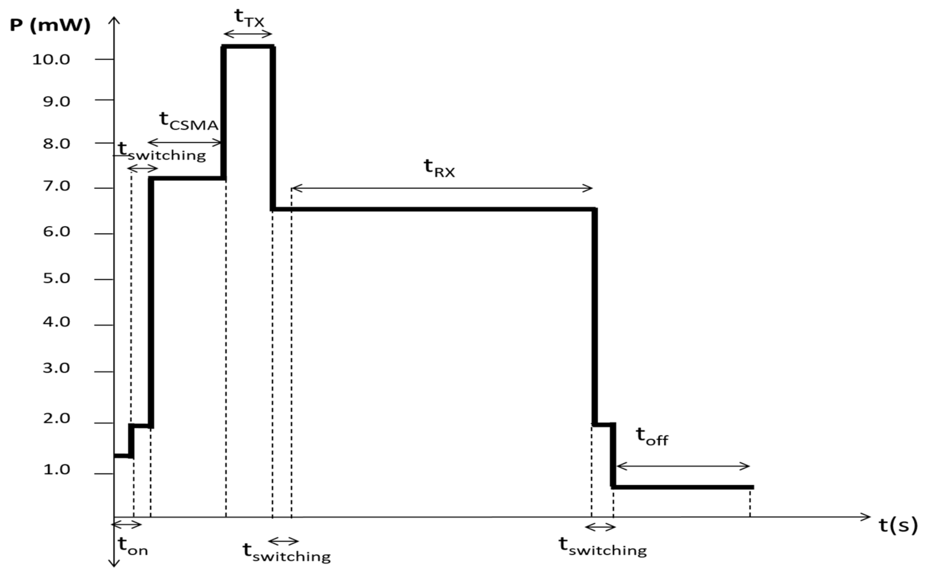
A WNS allows communication over a relatively short range of distances, which means that energy-efficient and low-cost solutions can be implemented in several systems. Energy models are used to show the network expenses in the main tasks of the nodes.

Table 4. Obtained energy model for the Zigbee sensor node [55].

Type of Energy	Energy (µJ)
Start-up mode	0.290
Switch from RX to TX	0.405
CSMA/CA algorithm	0.795
Radio in TX mode	5.975
Switch from TX to RX	1.285
Radio in RX mode	28.750
Shut down mode	1.525
MCU running on 32-MHz clock	0.985

and

Table 5. Obtained energy model for the WiFi sensor node [56].

Type of Energy	Energy (µJ)
Start-up mode	98.50
Switch from RX to TX	165.25
CSMA/CA algorithm	21.60
Radio in TX mode	925.50
Switch from TX to RX	165.25
Radio in RX mode	38.75
Shut down mode	615.0
MCU running on 32-MHz clock	0.24

show the energy models for both Zigbee and WiFi sensors, respectively, obtained from the carried out measurements. The main operating modes concerning the activities that a sensor node executes in the network represented the guidelines of the designed energy model. Initially, the node power on occurs at a start time (t_ON) (Figure 3). Then, the node takes a switching time (t_Switching) to modify its status before forwarding a data packet through the channel. Therefore, the node actuates the CSMA algorithm taking a specific CSMA time (t_CSMA). After, the node forwards the data packet for a specific time of transmission (t_TX). Still later, a switching time (t_Switching) is required by the node to modify the activity that it is running. It stays inactive (t_Inactive) and again modifies the task, taking a switching time (t_Switching) to start getting information and referring a reception time (t_RX). Each node executes these functions every time that it has to send and receive the data packets. Finally, the node switches off wasting a shutdown time (t_OFF). During this process, the micro-controller remains, all the time, in the active mode (MCU running on 32-MHz clock contribution in Table 4 and Table 5) Therefore, this temporal analysis allows determining the energy necessary for each activity performed by a node in the WSN.

As reported in Table 2 for the Zigbee sensor [55], the performed tasks and related time durations required for the whole process execution correspond to specific voltage and current values for each performed task, thus obtaining the total energy consumed by each node [54]. Then, Figure 3 outlines the time intervals of different operating phases, as described above, and related power consumption values, as reported in Table 2 for the Zigbee WSN node; so, we can refer to this graph for the calculation of the total energy, by using the following equation 1. Besides, in Table 4 and Table 5, we report the energy requirements, as obtained from the laboratory tests with Zigbee and Wifi sensors for the main activities of a node, in full agreement with values obtainable from Figure 3.

Therefore, the total energy can be determined using the following Equation (1):

$$E_{Total}=E_{MC}+E_{ON}+E_{OFF}+E_{CSMA}+E_{Switching}+E_{TX}+E_{RX}$$

(1)

3. Results

One of the objectives of this paper is to simulate a WSN under different types of routing protocols, analyzing the impact of performance metrics for each configuration accordingly. In this section, we want to bring the simulation conditions to a real scene with the distribution of sensors in an engineering building on a university campus. We want to compare the performance of two wireless technologies widely used in the telecommunications industry: Zigbee and WiFi. Likewise, four different routing protocols are implemented in the sensors in order to analyze the impact of each one on the wireless technology under study. In addition to the proposed protocols, in this work, three sleeping techniques are compared to observe the impact in each protocol.

3.1. Energy Analysis with the Sleeping Algorithms

Size and battery power are key features in energy consumption. By reducing the power consumption of each node, the overall energy requirement is reduced, thereby extending the battery life. Indeed, power management is supported at the MAC level for applications that use batteries. Features are provided in the communication protocol for stations or devices to go into sleep modality for a time interval defined by the coordinating node. Based on the need to optimize energy consumption, new research topics are being consistently introduced, such as energy collection and consumption optimization. In essence, reducing the power consumption of each node is equivalent to either turning off the device or letting it fall into sleep mode when it is not being used. In the sleep mode, all programs stop, and the microcontroller goes into a state of latency, from which it can be awakened by asynchronous interruptions. In other words, this mode makes it possible for the radiofrequency module to enter a low power consumption mode when it is not in use [57].

Indeed, the main advantage of sleeping techniques is the fact that each sensor only needs to be turned on in order to send data to another device; the rest of the time, it remains in a low power consumption mode. Accordingly, it is important to know the network tasks in which a node spends the most energy. Information of the tasks made by a node can be provided by the energy models that are proposed in this work because the main tasks of the nodes are described with an independent energy expenditure. Of course, sleeping techniques are not without their own problems: energy is used to wake the nodes. This is problematic since the microcontroller can never enter the deepest sleep state, because it always needs to leave at least one timer running in order to release the interrupts that determine the time slices and thus launch the scheduler. Besides, complete connections and disconnections of nodes generate reconfigurations in the topology, and it is here that routing protocol rules play an important role [58].

In this paper, we analyze two algorithms based on sleeping techniques, the first of which takes advantage of the routing tables of neighbors, which forms nodes according to the routing protocol. This mechanism, called the TSA, is shown in the flow-chart of Figure 4. In the TSA, HELLO packets bring extra information about the received signal strength indicator (RSSI) value of the source node; this data is then put into the neighbor tables when a classification of possible routes to a destination is made. In this way, when a node transmits a packet to the coordinator node, it chooses the optimal route (among its parents) based on the RSSI level; moreover, it only sends traffic packets to the said chosen node. A SLEEP packet with a proper timer is sent to the remaining possible nodes to reach the same destination. The nodes that receive the SLEEP packet put their MCU into sleep mode and activate the timer; in this way, when the timer ends, the nodes are in the active mode again where they can send and receive packets, and, accordingly, the overall energy of the network decreases. When a node is in the active mode, it resends a HELLO packet with its updated RSSI level so that its neighboring nodes update their tables. In this way, possible routes are optimized, energy is saved in the nodes, and route redundancy is maintained. However, this can be detrimental to the network with respect to the overhead, which will be compensated with the refresh of valid routes to the nodes in the network and link interference.

Another proposed algorithm is based on crowns, representing the location of the nodes regarding the coordinator node. Crowns are represented by hierarchical levels. The highest hierarchy is the coordinator node, followed by its neighboring nodes (directly connected), and so on. This system is well-known in the literature; for instance, [59] explains the workload and traffic generated by the nodes closest to the sink node. We propose a modification of this algorithm type based on sleeping techniques, wherein we establish the total number of nodes in the network and generate a percentage of nodes that can sleep for each hierarchy level; this algorithm is called MSC.

In the MSC Box 1, each node selects its neighbors according to the routing protocol. Besides, each node presents a hierarchy according to its proximity to the coordinating node, with the same hierarchy consisting of nodes that are directly connected to the coordinating node, and, subsequently, nodes connected to the latter have a lower hierarchy level, and so on. The nodes that have the same hierarchy form a crown. In this way, there are as many crowns as there are different hierarchies in the network. In each crown, a master node is chosen, which will have traffic information. A stable state period is established in the network, in which the topology is configured and the routing protocol runs normally. It is here that each node stores in its table the percentage information of its own traffic with respect to the network, which is passed on by the master node of each crown. Each master node organizes the information in an array, where it has the ID of each node with its respective traffic (which we call weight). Subsequently, each master node organizes the array based on weights in an ascending order regardless of the order of the node ID. The master node then creates a copy arrangement of the weights in order to create a new sleeping time arrangement for each node. This means that if a node has increased amounts of traffic, it will have less sleeping time.

Box 1. Pseudo-code of the MSC algorithm.

Start

Require: coordinator node start;

Set Hierarchy = 0

Initialize Hierarchy level of coordinator node = Hierarchy;

Initialize coordinator node establishes neighbors = i;

Hierarchy++;

Set neighbor_i establishes neighbors;

Calculate ncrown <- - nodes per crown;

Calculate weight [ncrown];

Calculate traffic_total;

for each crown do:

  Calculate weight_node_i = (traffic_node_i * 100)/traffic_total;

end for

Create pairs with ID and weights in ID_weight matrix

Create a copy of the weight array

Organize the weight_cpy array in ascending order

Create a matrix with IDs and weights in ascending order

Reorder the array weight_cpy in descending order

Insert the new descending array weight_cpy to calculate the sleeping time for each ID

end

Now, we present the two real networks implemented in this work. First, the description of the two networks is presented, and then the energy model for the routing protocols is described. The sensors are located in the engineering building of Universidad Panamericana, Guadalajara, Mexico, which has an area of approximately 300 × 300 m². This scenario represents an ideal pedestrian and vehicular traffic environment almost every weekday. Accordingly, many devices can cause interference, such as computers, cell phones, and laboratory equipment. Besides, the building is also surrounded by nature and other buildings, such as coffee shops and car parks. This scenario is shown in Figure 5. The areas of the building that are numbered are described below: (1) Computer laboratories with 60 computers; (2) Patio and open area; (3) Professors’ offices; (4) Cleaning room and electrical connections; (5) Laboratories of physics, product design, and civil engineering; (6) Laboratory of measurements.

3.2. Description of the Real Implementation of the Networks: Zigbee and WiFi

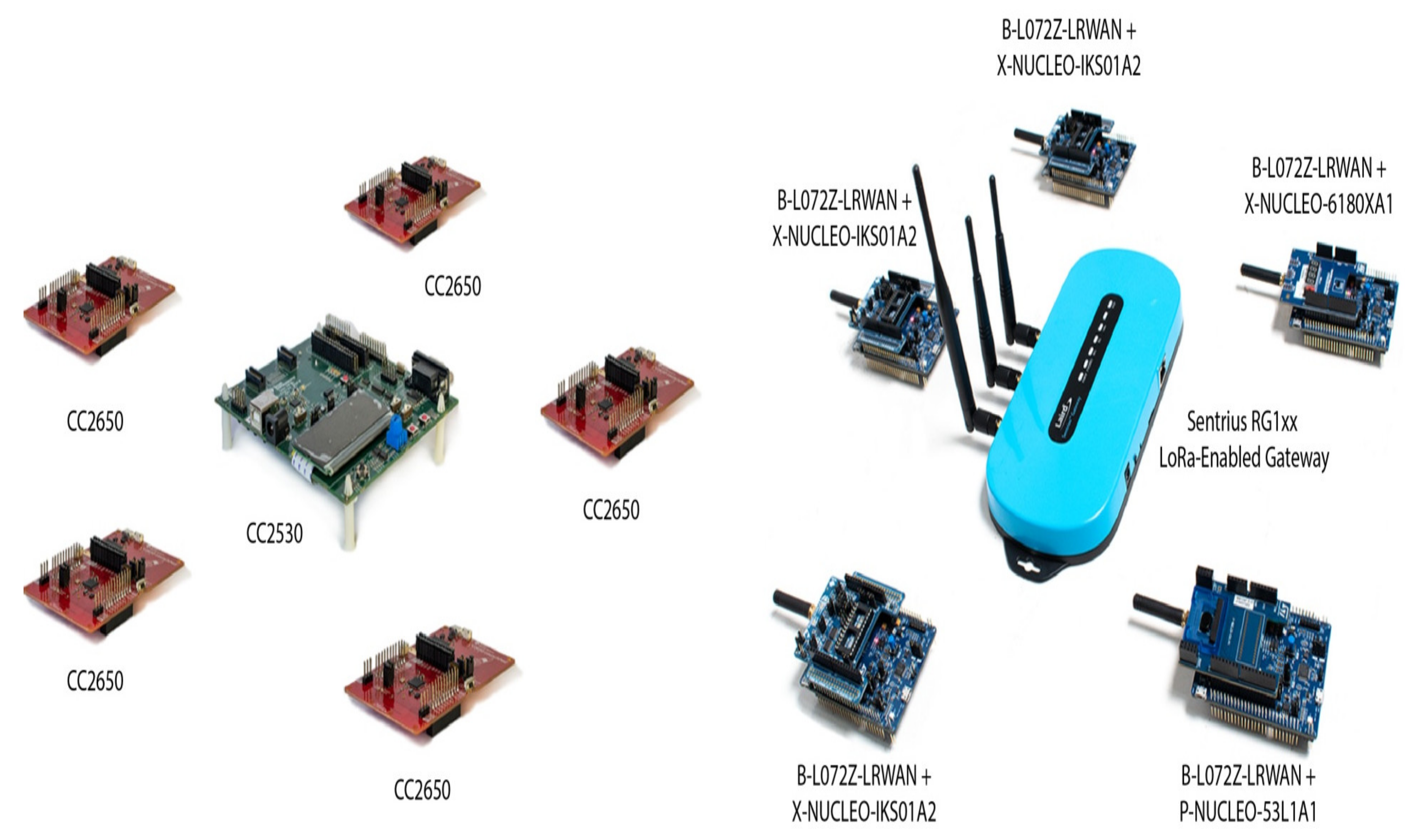
We implemented a real scenario as shown in Figure 6. This Figure shows a sensor network composed of long-distance ranging sensors, data acquisition, and computing electronic boards and a gateway, whose technical features are detailed below.

√

Sentrius RG1xx LoRa-Enabled Gateway (manufactured by Laird Technologies Inc, Chesterfield, MO, USA):

• Secure, scalable, and robust.
• It can gather data over LoRaWAN or Bluetooth and send them as far as 10 miles via LoRaWAN, or over WiFi/Ethernet to the cloud.
• It gives full ownership over the network, adding multi-protocol connectivity to the sensors and devices to get actionable IoT intelligence [60].

√

STM B-L072Z-LRWAN electronic board (manufactured by ST Microelectronics Co., Geneva, Switzerland):

• It is an evaluation card, based on the Arm Cortex-M0+ microcontroller that supports the protocols LoRaWAN, Sigfox and LPWAN as well as ARM Mbed, Atollic as development tool.
• It can be powered from the USB or by AAA batteries.

√

STM X-NUCLEO-IKS01A2 expansion card (manufactured by STMicroelectronics Co., Geneva, Switzerland) [56]:

• It is a motion MEMS and environmental sensor expansion board for the STM32 X-Nucleo board.
• It has onboard environmental and movement sensors (LSM6DSL 3D accelerometer and 3D gyroscope, LSM303AGR 3D accelerometer and 3D magnetometer, HTS221 humidity, and temperature sensor, and the LPS22HB pressure sensor).
• It is equipped with Arduino UNO R3 connector layout.

√

STM P-NUCLEO-53L1A1 evaluation card (manufactured by STMicroelectronics Co., Geneva, Switzerland) [56]:

• It allows measuring long distances independently of target reflectance by using two VL53L1X Time-of-Flight (ToF) long-range distance sensors;
• The connection to the STM32F401RE Nucleo board provides a flexible way to build new prototypes.

√

STM X-NUCLEO-6180XA1 expansion board (manufactured by STMicroelectronics Co., Geneva, Switzerland) [56]:

• It is a module for detection of proximity, gesture, and ambient light (ALS) based on STs FlightSense™ and Time-of-Flight technologies (VL6180X sensing module);
• Slider that controls two functions: (1) Range measurement, beyond 400 mm; (2) Detection of ambient light, up to 100 kLux;
• 4-digit display related to the distance of a target from the proximity sensor or the lux value from ambient light detection.

In this experiment, six nodes were used: five nodes were given a star topology, and to another one the coordinator function. This layout is shown in Figure 6. For creating the Zigbee network, the coordinator node has to be the CC2530 Zigbee module because the flashing of the CC2650 electronic board is not sufficient to build the WSN. CC2650 LaunchPad has the following components on-board: an 8 Mbit serial flash for allowing any over-the-air firmware updates, two push-buttons, an evaluation module, two light-emitting diodes, two Booster-Pack connectors, and a LaunchPad XDS110 debugger. Besides, the 802.15.4 protocol has been employed, an easy-link protocol for making networks and transmitting data at 2.4 Ghz frequency. To be sure, for acquiring the Zigbee packets, it has been used the CC2650 board as a sniffer. Besides, the CC2530 Zigbee-based node was employed as the coordinating device. The evaluation board that was used to program this node was the TI SmartRF05 one (manufactured by Texas Instruments Co., Dallas, TX, USA), consisting of different inputs and outputs. If the device is in the idle state, any interruptions result in the device returning to the active state. Moreover, some interruptions can result in the device waking up from the sleep mode.

3.3. Comparison between the Simulation Tool and the Real Scenario

The models described in Table 4 and Table 5 were used for simulating the networks with the same number of sensors, as depicted in Figure 6. They were tested by using the MPH, AODV, LEACH, and ZTR protocols. Afterward, the same scenarios that we simulated through the developed simulator, were implemented by using real sensors, and the code parameters were changed properly in order to employ, one after another, the MPH, AODV, LEACH, and ZTR protocols. One day simulations were conducted with the same conditions specified in Table 1 for all the cases.

It is important to note that the protocols that we are going to take into account are exemplary in this work, AODV (reactive), MPH (hybrid), LEACH (energy-aware), and ZTR (proactive), in order to compare different natures for reconfiguration of the links against to changes in the network.

Table 6. Energy comparison.

	Model with the CC2650 Sensor Nodes Time (µs)
	ZTR Energy (J)	MPH Energy (J)	AODV Energy (J)	LEACH Energy (J)
Simulation	0.019279	0.019834	0.041575	0.018334
Real scenario	0.019165	0.019745	0.041342	0.018951
	Model with the X-NUCLEO Sensor Nodes
	ZTR Energy (J)	MPH Energy (J)	AODV Energy (J)	LEACH Energy (J)
Simulation	0.026872	0.027765	0.058367	0.028361
Real scenario	0.026776	0.027037	0.059173	0.029281

shows the energy comparison between the simulations and the real scenario. These tests were conducted in order to extrapolate the behavior and the quantity of the nodes, as well as to ensure that the network grows so that at any given time, we have an intelligent building, but later, we can apply it to an intelligent campus and analyze performance conditions of the two wireless technologies widely used.

The behavior of the simulation model is comparable to the actual behavior of the sensors: 1.2% error for the CC2650 sensor model and an error of 0.7% for the X-NUCLEO sensor model. In addition, the results suggest that the energy consumption of the MPH is similar to ZTR. In particular, ZTR expends 6% less energy than the MPH one, which is significant because MPH is a complete routing protocol with higher scalability and redundancy. The protocol with the worst energy performance is AODV, which in the CC2650 tests, consumes roughly 20% more energy than the other protocols; besides, in the X-NUCLEO tests, it consumes 40% more. We note that the LEACH protocol has an energy saving capacity on a reactive protocol such as AODV of 56%; instead, it only presents an energy saving of 6% compared to MPH and ZTR, which are protocols with similar behaviors. LEACH is advantageous over AODV concerning the number of hops and the master node information handling, which become intermediate base stations to reach the coordinator. Indeed, the AODV has a large number of control packets, a mesh configuration, and route requirements when they do not exist or become obsolete. This generates some overhead in the network as well as a large number of collisions that reduce the network life.

Table 7. Effective sent and lost messages: Packet Delivery Ratio (PDR).

	Model with the CC2650 Sensor Nodes
	ZTR PDR (%)	MPH PDR (%)	AODV PDR (%)	LEACH PDR (%)
Simulation	80.3	95.4	92.8	94.3
Real scenario	81.2	94.9	92.0	94.5
	Model with the X-NUCLEO Sensor Nodes
	ZTR PDR (%)	MPH PDR (%)	AODV PDR (%)	LEACH PDR (%)
Simulation	86.7	97.3	95.5	96.6
Real scenario	86.4	96.2	96.0	96.9

shows the Packet Delivery Ratio (PDR) rate in percent related to each analyzed power protocol, in the two network configurations shown in Figure 6. The two implemented network models differ by 7% in terms of the number of packets arriving vs. the packets sent per node on average. The WiFi model presents better performance, possibly due to the capacity and directionality of the antennas and the management of packets by the gateway. Regarding the routing protocols, ZTR has a 16% higher loss of information due to low redundancy on the links, while MPH, AODV, and DSR differ by only 2%, in favor of MPH. It has a higher topology reconfiguration capacity, and the link redundancy is acceptable. AODV and DSR are probably highly responsive due to their reactive nature, but poor reconfiguration due to the number of control packets.

3.4. Interference Impact on the Sleeping Algorithms

Different factors affect the operation of WSNs, which in turn, depend on various aspects of the network itself, such as the technology used by the device, the signal environment, and the physical laws of wireless transmission [61]. Interference in the sensor networks determines the strength with which the signal is received as well as the intermittency of the packets for information delivery. Indeed, WSNs are becoming more and more common, which means that there are more and more wireless transmissions in the air. Signals that operate on the same frequency often interfere, with negative effects on performance. This means that the 2.4 GHz free band, which is the most used band, can be severely affected by other signals to the point where a device will not work with acceptable performance metrics [62].

Wireless networks can support more than one communication with the same coordinating node at the same time. This implies that a bottleneck is created when there is an increase in the client devices on the same network, since the access point must instantly communicate with all of them. Besides, if there is an increase in users on the same network bandwidth, then less information can be shared between them, and, accordingly, interference between devices weakens the signal, generating collisions and packet losses. In the following Figure 7, Figure 8, Figure 9, Figure 10, Figure 11 and Figure 12, we analyze the RSSI parameters, which is a measure of how well a device can detect and receive signals from any access point. Indeed, the closer the value approaches zero, the stronger the signal will be.

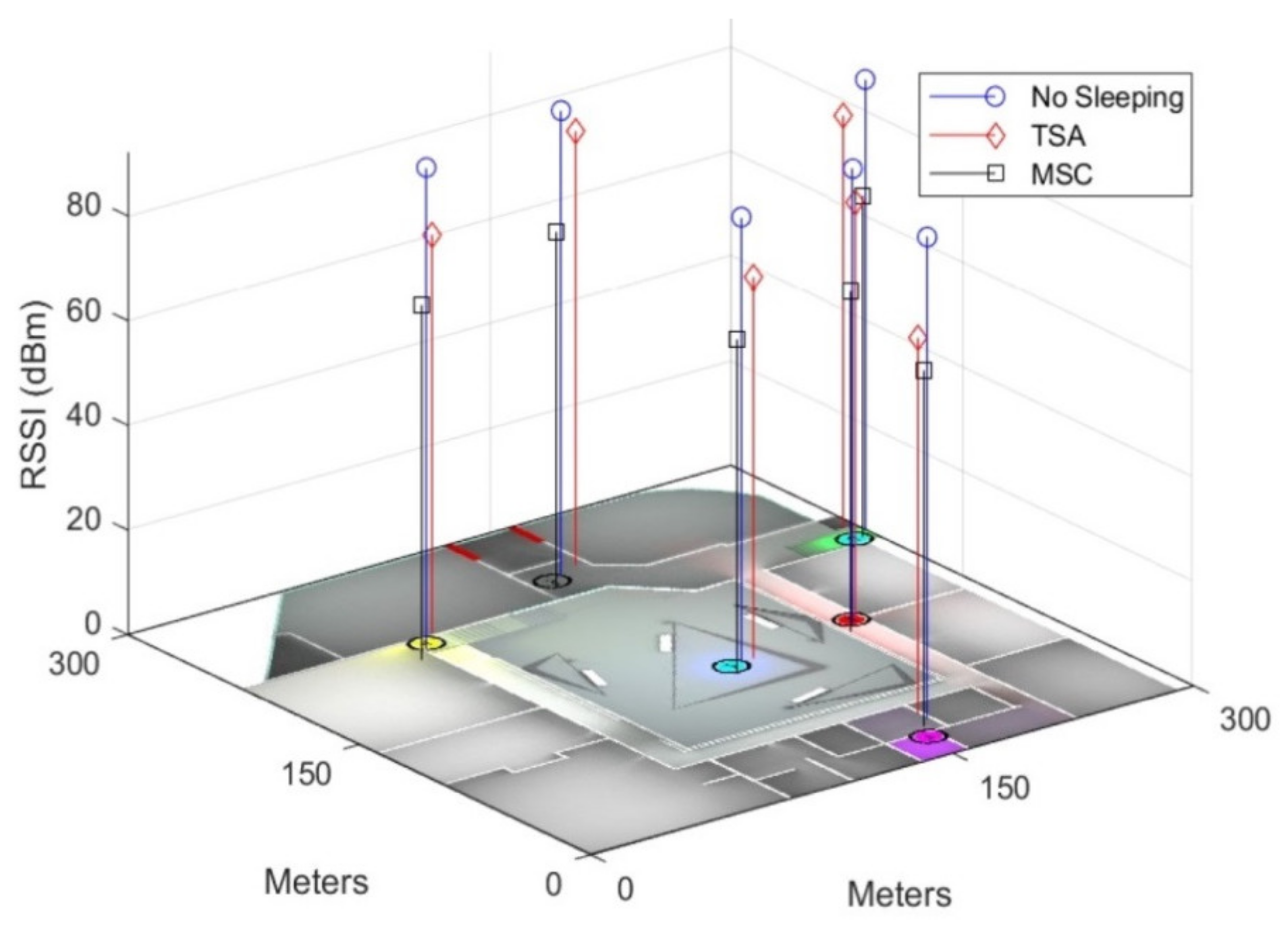
For these results, sensors in Figure 6 for both Zigbee and WiFi were placed in the positions shown in Figure 5 in a university campus building in the city of Guadalajara, Mexico. Tests were conducted over 7 days, with measurements taken every hour; these measurements were then averaged, thereby obtaining the final results. The star topology feature of WiFi networks requires that all devices react to signals from the controller, even if only one of the devices is being consulted. The energy balance of this system is that each query involves energy consumption for all network devices. It is for this reason that we decided to compare the actual consumption of both technologies in a real scenario with the same data rate conditions, radio signal levels, transmission intervals, and different types of widely known communication protocols: AODV, LEACH, and MPH.

Each of these protocols has different characteristics concerning the number of control packages (overhead) and reconfiguration of the network topology. For each protocol, both wireless technologies were tested: Zigbee and WiFi. The average difference between these two technologies is approximately 9% in favor of Zigbee, suggesting that Zigbee has less signal interference in almost all nodes. In particular, for Zigbee, the difference is 10% in favor of LEACH with respect to AODV, 6% in favor of MPH with respect to AODV, and 4% in favor of LEACH with respect to MPH. Alternatively, for WiFi, the difference is 20% in favor of LEACH with respect to AODV, 23% in favor of MPH with respect to AODV, and 3% in favor of MPH with respect to LEACH.

Concerning the comparison of the proposed sleeping techniques, we have the following analysis. The average difference between no sleeping and TSA is 8% better signal when the TSA algorithm for Zigbee is present in the nodes under the AODV protocol. Under the same conditions mentioned above, when the MSC algorithm is present, the signal is optimal at 16%. In addition, MSC is 9% better than the TSA. Under Zigbee, with respect to the LEACH protocol, we have an increase in the signal strength of 6% for TSA and 20% for MSC. Besides, MSC has a better signal at 12% compared to TSA. Similarly, for Zigbee, with respect to the MPH protocol, we have 18% in favor of TSA versus no sleeping and 26% in favor of MSC versus no sleeping; moreover, MSC improves the signal by 11% compared to TSA.

Analyzing the WiFi technology, for AODV, the TSA algorithm represents greater signal strength by 13% compared to no sleeping technique, MSC has 23% in favor of not sleeping, and MSC has a better signal at 13% compared to TSA. With respect to LEACH, TSA has a better performance compared to not sleeping at 16%; moreover, MSC has 11% in terms of a greater signal strength than TSA. Finally, with respect to the MPH protocol, the TSA algorithm is better by 14% with respect to the network when there are no sleeping nodes; moreover, MSC has a signal strength of 26% versus no sleeping, and it is 14% better compared to TSA.

3.5. Local Energy Information (LEI) Algorithm

We generated a simple algorithm wherein each node in the HELLO packet sends information about total energy consumption, and the source node stores this information in the neighbor table for each node ID. This simple proposed algorithm is rigid with respect to the way each node should adopt information. It is for this reason that we have not compared it with the other two algorithms presented in this paper: TSA and MSC are more complex algorithms that require a greater amount of processing. Graphically, the states that the nodes can take are shown in Figure 13, Figure 14 and Figure 15 for the six nodes that are used in this paper. This algorithm is called the local energy information (LEI) algorithm because several of the techniques proposed in the literature [63,64] are based on sleeping a percentage of nodes or keeping them in active mode according to the energy expenditure in the network. We propose this algorithm in order to scale the network and increase the number of nodes to now compare the three sleeping techniques that are proposed in this work.

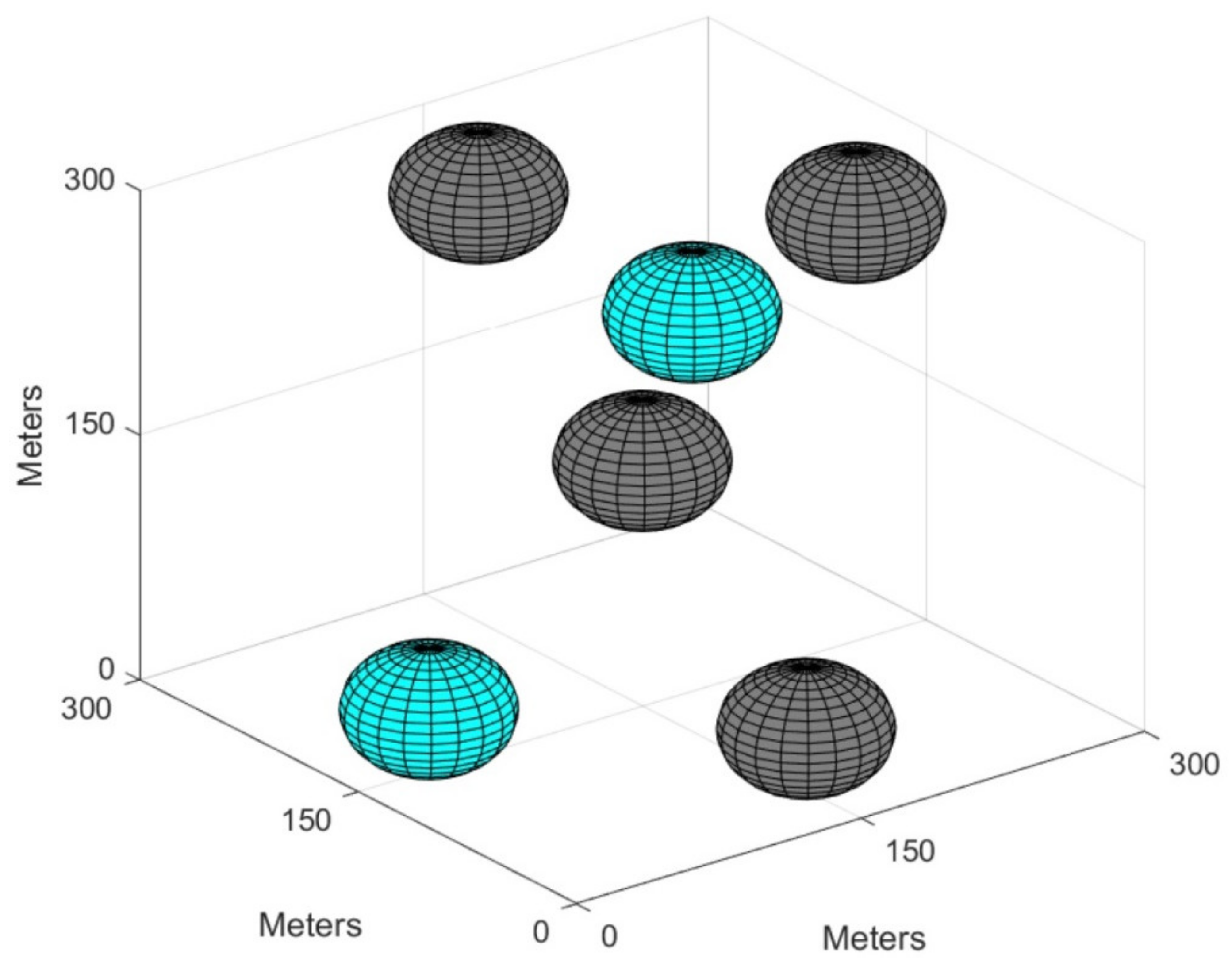
With the scheme of these figures, we intend to visually the state of the nodes: active or sleep mode. The figures show the area of the campus engineering building comprised of 300 square meters. The spheres represent the nodes located in the studied scenario. The different colors of the spheres represent that the nodes are in different states during the simulation time. The LEI algorithm is based on timers to sleep the nodes. Therefore, we wanted to evaluate the three possible states in which the nodes were distributed in the network.

We have two possible energy states for a node: active mode and sleep mode. Remember that for the sleep mode, a timer is activated and it starts running and when the time is over, the node returns to active mode. Figure 13, Figure 14 and Figure 15 show the possible states in which a network can be found. Figure 13 shows a representation of when one node is in a sleep state, and the others are in the active mode. Figure 14 shows when two nodes remain in active mode, and four nodes are in sleep mode. Figure 15 also represents four nodes in sleep mode, but with different timers and two nodes in active mode. These are the three possible scenarios to analyze according to the scheme of Figure 6.

In a network of six nodes, which is the sample of our real scenario, we can find different moments in which the nodes can be found in active mode or sleep mode. Figure 13 shows the “worst” scenario because 84% of the network nodes is in active mode, and only 16% is in sleep mode. This scenario constitutes the highest energy consumption. Now, in Figure 14, we have 66% of nodes in sleep mode and 33% of nodes in active mode. In Figure 15, we have the same scenario as in Figure 14, with the difference that the nodes that are in sleep mode have a time lag and that two nodes will change state after two other nodes. The advantage of this LEI algorithm strategy is that the nodes change state according to the needs of the network, and asynchrony provides an added value to the optimization of the energy in the nodes. Quantitatively, the scenario in Figure 13, during 24 h of continuous experimentation, yields 0.056 J for Zigbee and 0.064 J for WiFi. The scenario in Figure 14 shows 0.051 J for Zigbee and 0.059 J for WiFi. Finally, the scenario in Figure 15 shows 0.048 J for Zigbee and 0.056 J for WiFi. This shows that the distribution of timers provided by the LEI algorithm, when the nodes have asynchronous state change modes, has an energy gain of 13% for the network.

Table 8. Energy behavior per each studied algorithm under MPH protocol.

ZIGBEE Configuration
TSA		MSC		LEI
Energy per Node (J)	Total Energy (J)	Energy per Node (J)	Total Energy (J)	Energy per Node (J)	Total Energy (J)
0.008123	0.025254	0.006924	0.018894	0.009431	0.042381
WIFI Configuration
TSA		MSC		LEI
Energy per Node (J)	Total Energy (J)	Energy per Node (J)	Total Energy (J)	Energy per Node (J)	Total Energy (J)
0.009662	0.030821	0.008667	0.027454	0.013186	0.050163

,

Table 9. Energy behavior per each studied algorithm under AODV protocol.

ZIGBEE Configuration
TSA		MSC		LEI
Energy per Node (J)	Total Energy (J)	Energy per Node (J)	Total Energy (J)	Energy per Node (J)	Total Energy (J)
0.009463	0.027135	0.007653	0.020864	0.010273	0.045643
WIFI Configuration
TSA		MSC		LEI
Energy per Node (J)	Total Energy (J)	Energy per Node (J)	Total Energy (J)	Energy per Node (J)	Total Energy (J)
0.011194	0.034382	0.009763	0.029564	0.016234	0.053582

and

Table 10. Energy behavior per each studied algorithm under LEACH protocol.

ZIGBEE Configuration
TSA		MSC		LEI
Energy per Node (J)	Total Energy (J)	Energy per Node (J)	Total Energy (J)	Energy per Node (J)	Total Energy (J)
0.007653	0.024193	0.005538	0.017163	0.008234	0.041153
WIFI Configuration
TSA		MSC		LEI
Energy per Node (J)	Total Energy (J)	Energy per Node (J)	Total Energy (J)	Energy per Node (J)	Total Energy (J)
0.009023	0.029845	0.007473	0.026123	0.012248	0.048274

have simulation times of one day (24 h) and the algorithms can be tested with any protocol: reactive (AODV), energy-aware (LEACH), or hybrid-proactive (MPH). We tested the energy saving techniques with 100 nodes and we ran the two technologies studied: Zigbee and WiFi. Analyzing the results of Table 8, Table 9 and Table 10, we obtain that the energy expenditure for these different network types is, on average, 15% higher for the WiFi network compared to the Zigbee one. However, for the MPH protocol under Zigbee technology, the energy expenditure is 36% higher for LEI compared to MSC, 41% compared to TSA, and 25% more energy expenditure with the TSA compared to MSC. In the same protocol analysis for WiFi wireless technology, LEI spends 46% more energy than MSC, 39% more energy compared to TSA, and MSC 11% more energy compared to TSA. For the AODV protocol for the Zigbee technology, LEI has an expense of 55% against MSC and 41% against TSA, and between MSC and TSA there is a difference of 23% in favor of MSC. Now, under WiFi technology, LEI spends 45% more energy than MSC and 36% more than TSA; besides, between MSC and TSA, there is a difference of 14% in favor of MSC. Finally, for the LEACH protocol under the Zigbee technology scheme, LEI has a higher expense of 59% compared to MSC, 42% compared to TSA, and finally between TSA and MSC, the TSA exhibits a 29% higher consumption than MSC. Under WiFi for this protocol, we have that LEI spends 46% more energy than MSC and 38% more than TSA, and finally between MSC and TSA the difference is 12% in favor of MSC. Nevertheless, we observe that compared to LEI, the gain of the MSC algorithm is around 43%, which indicates that there should be an intelligent organization to sleep the nodes in a wireless network. The LEI algorithm leads to sleep only node with respect to its use (average energy consumption), but this is a light decision-making. MSC compares the local traffic of a node and this becomes a proportional sleeping time value, which is a more intelligent decision: choosing a node that becomes asleep.

4. Discussion

Finally, in this section, we discuss some performance metrics that directly impact energy consumption, such as Resilience and Packet Delivery Ratio. We analyze the typical and atypical sleeping techniques studied on the mentioned protocols. In addition, we compare topologies commonly used in sensor networks to analyze the efficiency of packet delivery between WiFi and LoRa. The impact of this work focuses on the comparison of routing protocols of different nature, implemented for the widely used wireless technologies. Moreover, the originality of this comparison lies in the application of sleeping techniques in real sensor network scenarios and the analysis of performance metrics that directly influence the energy consumption of the network.

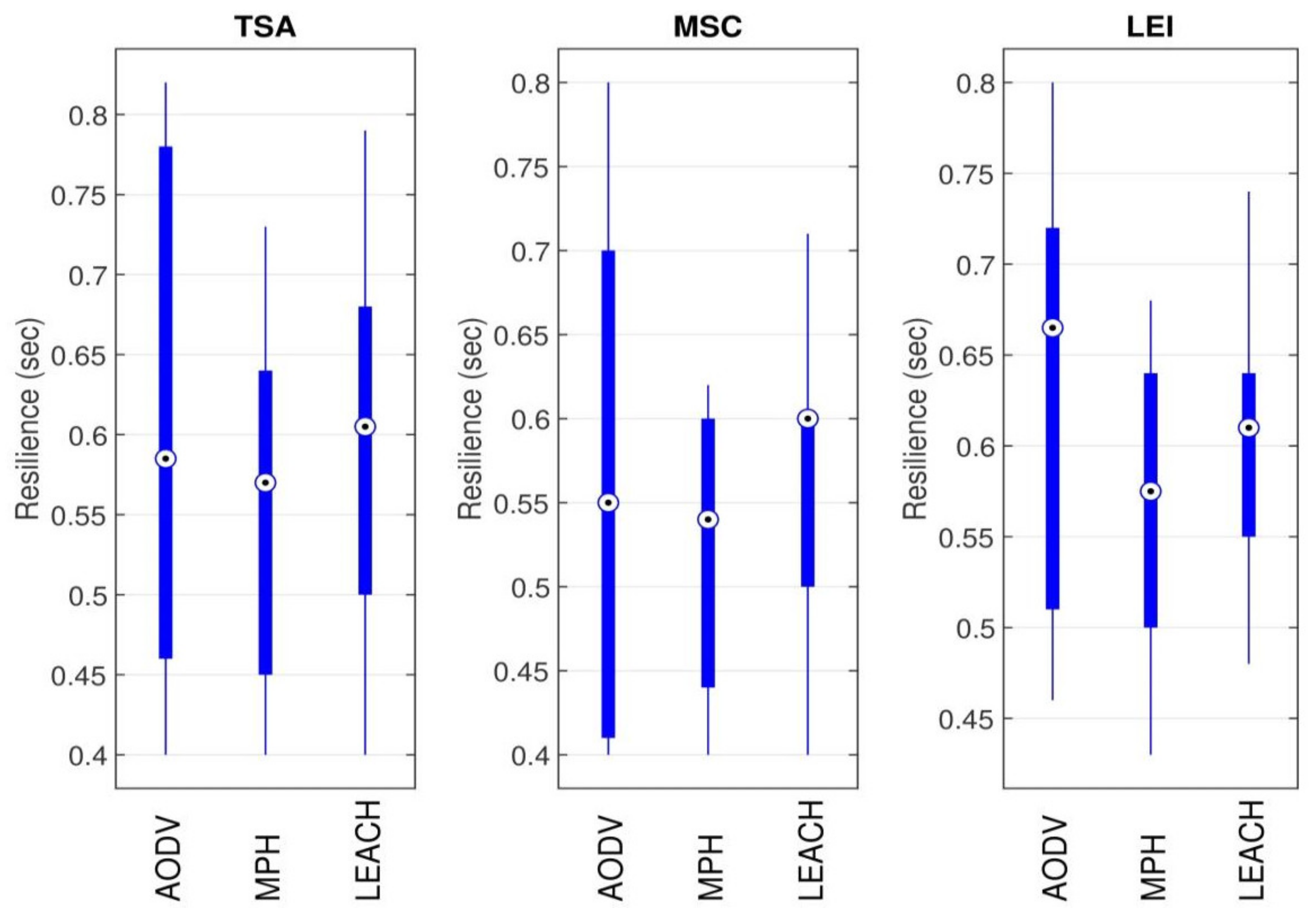
Figure 16 and Figure 17 show the resilient behavior of the three techniques exposed in this work (TSA, MSC, and LEI) for three representative protocols, both for LoRa and for WiFi. The results are taken every 6 h for seven days, starting from Monday and ending on Sunday. We choose a reactive protocol (AODV), a hybrid protocol (MPH), and an energy-aware protocol because we want to check how long each one takes depending on the sleeping technique used. LoRa and WiFi are two wireless technologies that have been quite contrasted in recent times because WiFi represents the reliability and compatibility of equipment, and LoRa represents novelty, versatility, and efficiency. The difference in this performance metric shows that LoRa represents a 37% better resilience against WiFi, which means that LoRa takes less time to reconfigure the topology of the nodes in the face of an unexpected event, such as sleeping a sensor. Or several (according to the sleeping scheme). We note that AODV is the least resilient protocol at an average of 11% against MPH and LEACH. However, the most efficient technique remains MSC with a difference of approximately 13% against TSA and 28% against LEI. The meaning of applying a Box Whiskers scheme for this type of result is to observe the dispersion of the results and the average recovery time for each protocol in each sleeping technique. As the filled rectangle becomes shorter, the data moves at values close to the range indicated by the y-axis of the graph. The extreme values, represented as circles, denote outliers of recovery times that are very different from the average. The behaviors of the network on Saturdays and Sundays, in which there is less presence of staff and students on campus, can contribute to these outliers. The thin bars that accompany the rectangle (whiskers) are the total interval in which the data moves. The AODV protocol shows a longer interval, observing outliers in which the recovery of the network topology is not very good.

Although WiFi sensors have higher energy expenditure than Zigbee (Table 4 and Table 5), it is essential to mention that Zigbee protocols have less link redundancy. There are no links between nodes in the same hierarchy, and they only allow one parent per node. While WiFi sensors create a mesh topology network with highly redundant links, this difference makes the number of packets lost for Zigbee higher than for WiFi. Therefore, the number of re-transmissions and attempts to listen to the channel increases, and this affects the energy consumption. For this reason, the impact on the difference between the values of the power models for WiFi and Zigbee (in favor of Zigbee) is compensated by the loss of packets due to the low redundancy in routes for the Zigbee sensors [65,66].

Implementation under Different Topologies

LoRa is an ideal technology for connections over long distances and for IoT networks where sensors that do not have mains electricity are needed, with high applications for Smart Cities, in places with little coverage or to build private sensor networks and/or actuators. WiFi is one of the best known and adopted technologies. Among its main advantages is a large capacity for data transfer, which allows sending video, audio, and other large files. One of the significant disadvantages of this technology is the scope of coverage, although it is possible to make point-to-point links of several kilometers, for sensor networks where it is necessary to have a multi-point connection.

In Figure 18a, we implement star, bus, and mesh typologies for the MSC technique and WiFi technology under the hybrid MPH protocol. We observe the rate of packets delivered satisfactorily on average for each of the hours of a day of the week (Wednesday). We choose this day because the activities on the university campus are normally carried out, both of the people who work there and of students and operators. The measurement described here is an average of data collection during ten Wednesdays for each hour of the day. We perform three logical topology tests for the distribution of nodes that we have in the engineering building: star, bus, and mesh. We note that the logical topology that presents the highest satisfaction of packet delivery is the star, with 5% more packets delivered in front of the bus topology and 10% with respect to the mesh topology. Between the bus and mesh topology, there is a difference in the delivery of 5% packets in favor of the bus topology.

As we describe in Figure 18a for WiFi and in Figure 18b for LoRa, we present the results under the MPH protocol. The best performing topology for LoRa links is the mesh with a difference of 9% from the star topology. Also, the difference between mesh and bus is 12% in favor of the mesh topology. This behavior may be due to the fact that the mesh topology presents greater redundancy in its links for LoRa and not in the case of WiFi. This difference (under the same experimentation conditions) is because that LoRa has high interference tolerance (even higher than WiFi) and high sensitivity to receive data, which could cause the topology, which is, par excellence, more robust (mesh) is optimal in this case.

5. Conclusions

Wireless technologies advance rapidly every year and their use has become indispensable to managing different systems at the lowest possible cost. The WiFi protocol has been improved to have both a better range and transmission speed. WiFi has great competition in wireless technologies such as Zigbee; a wireless communication system focused on communication between devices with a low data rate to have the lowest possible energy consumption. This work compares the performance of WiFi and Zigbee protocols under the same scenarios and parameters, and it is evident that Zigbee has a 15% energy saving in several widely known communication protocols. However, it is important to observe the impact on various protocols because drastic changes occur in a network, such as connections and disconnections of nodes, reconfigurations, latency, retransmissions, and other metrics that can degenerate the performance.

In this work, we analyze the energy impact using different types of routing protocols: proactive (ZTR), reactive (AODV and DSR), hybrid (MPH), and energy-aware (LEACH). The results for MPH protocol are encouraging, because it performs well in the information processing and efficient data delivery as well as in the energy saving. AODV and DSR are very efficient in terms of backup paths and node-to-node connectivity because they form a mesh network. ZTR is a quick algorithm with low power consumption, but it is not very reliable in unfavorable network conditions or links failures, neither it is a resilient protocol. Based on the reported results related to the two widely used wireless technologies, Zigbee has an energy saving of around 8% compared to WiFi. Likewise, comparing routing protocols of different nature, we found that a hybrid protocol such as MPH exhibits 4% lower power consumption compared to a simple proactive protocol such as ZTR; and 15% less consumption compared to a reactive protocol such as AODV, and 6% less consumption compared to a well-studied protocol of an energy-aware nature such as LEACH. In addition, the sleeping techniques analyzed in this work show better energy consumption for MSC of 6% concerning TSA and 13% toward LEI.

The mix of a hierarchical topology with the self-configuration mechanism of the MPH protocol, allows nodes to perform the network processes, reduce the delays, take short routes to the destination, get back the network topology faster, and reduce the network overhead. Consequently, these characteristics lead to successful data delivery and, at the same time, low energy consumption. One of the most efficient protocols is LEACH, which is based on the division of network nodes into clusters and the choice of a set of master nodes based on a probability, which exerts this role for a certain time. This results in shorter jumps toward the successful delivery of the information. The difference in performance, based on metrics (retransmissions, listening retries, resilience, interference, and others under study in this work) shows that the difference between MPH and LEACH is about 4%. MPH is also a complete protocol of a hybrid nature (proactive and reactive) that establishes nodes hierarchies. These features make this protocol good enough to optimize network resources. The routing protocols are implemented in a real network in the Engineering building of the Universidad Panamericana in Guadalajara, Mexico.

Finally, an energy analysis that compares an existing algorithm with two new sleeping algorithms (proposed and described in this work) is reported. The tests were performed using three different energy models; in all cases the MSC algorithm had a better energy performance regarding TSA, approximately 12%. In addition, these two proposed algorithms are more efficient in energy consumption by 45% compared to the algorithms of the literature based on sleeping nodes under absolute consumption schemes.