Multiple Site Intraday Solar Irradiance Forecasting by Machine Learning Algorithms: MGGP and MLP Neural Networks

 ,
,  , ,
, ,  ,
,  and
and 
Abstract

1. Introduction
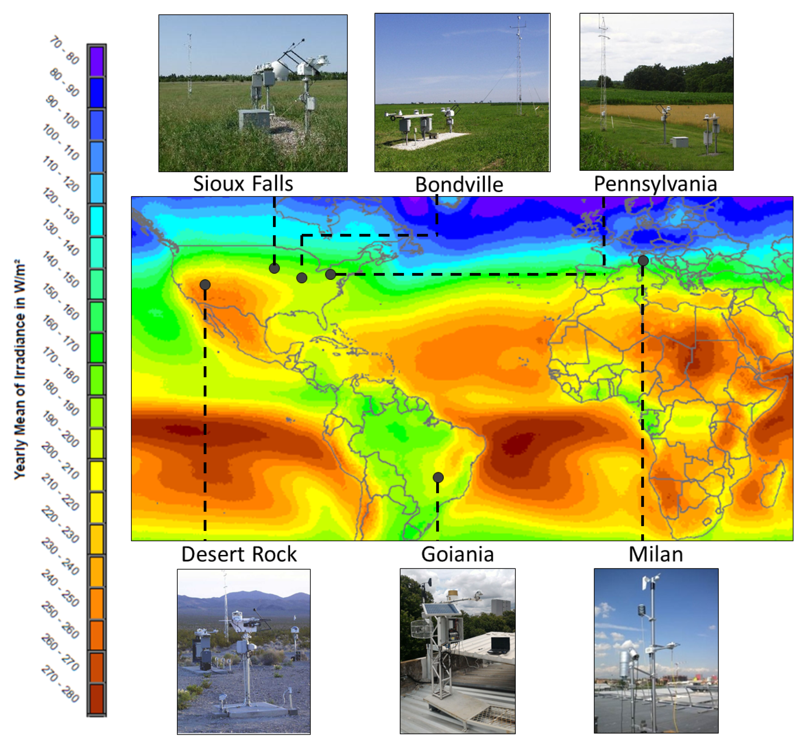
2. Databases
2.1. Goiania, Brazil
2.2. Milan, Italy
2.3. SURFRAD-US
3. Data Processing
3.1. Normalization
3.2. Data Statistics
3.3. Data Relations
- -
- (-5)…(-60): the 12 past values of in time windows of 5 min averages.
- -
- (-5)…(-60): the 12 past values of ambient temperature in .
- -
- (-5)…(-60): the 12 past values of wind speed in m/s.
- -
- (-5)…(-60): the 12 past values of relative humidity in %.
- -
- (-5)…(-60): the 12 past values of atmospheric pressure in mBar.
- -
- h is the elevation angle of the forecast time window in radians, varying from around 0.0873 (5) to 1.5708 (90).
- -
- is the time difference in respect to sunrise in minutes.
- -
- is the solar time angle in radians.
- -
- “Day” is the day of forecast interval. The days of the year are counted starting one day after the winter solstice and ending on the winter solstice of the next year. We decided to adopt this definition to follow the solar cycle starting from the day of lowest irradiance levels, since the traditional day counting does not have a direct mathematical relation to the evolution of solar variables throughout the year.
- -
- “Month” is the month of the forecast interval, varying from 1 to 12.
4. Forecast Methods
4.1. Genetic Programming
| Algorithm 1: Genetic programming pseudocode |
 |
4.2. Artificial Neural Networks
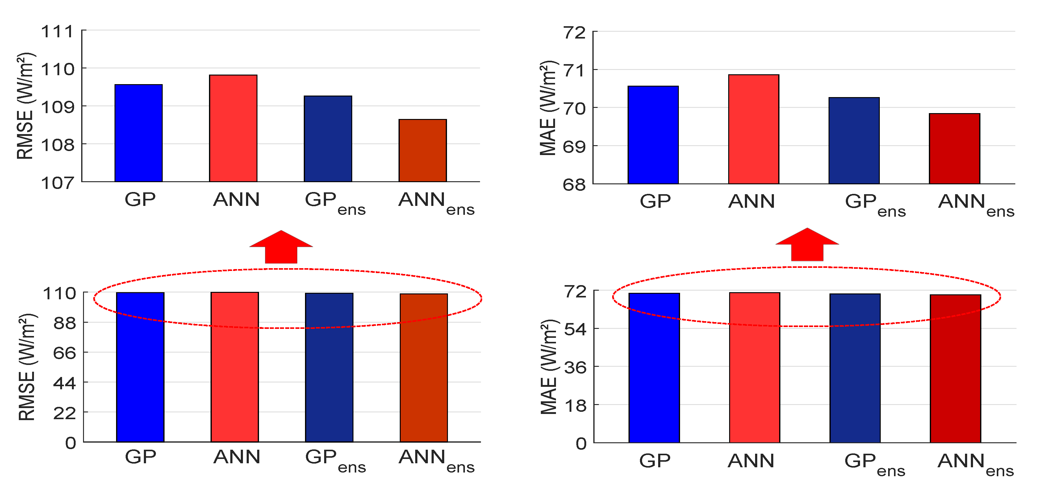
4.3. Ensemble Forecasts
4.4. Iterative Forecasts
4.5. Persistence
5. Error Metrics
6. Results and Discussion
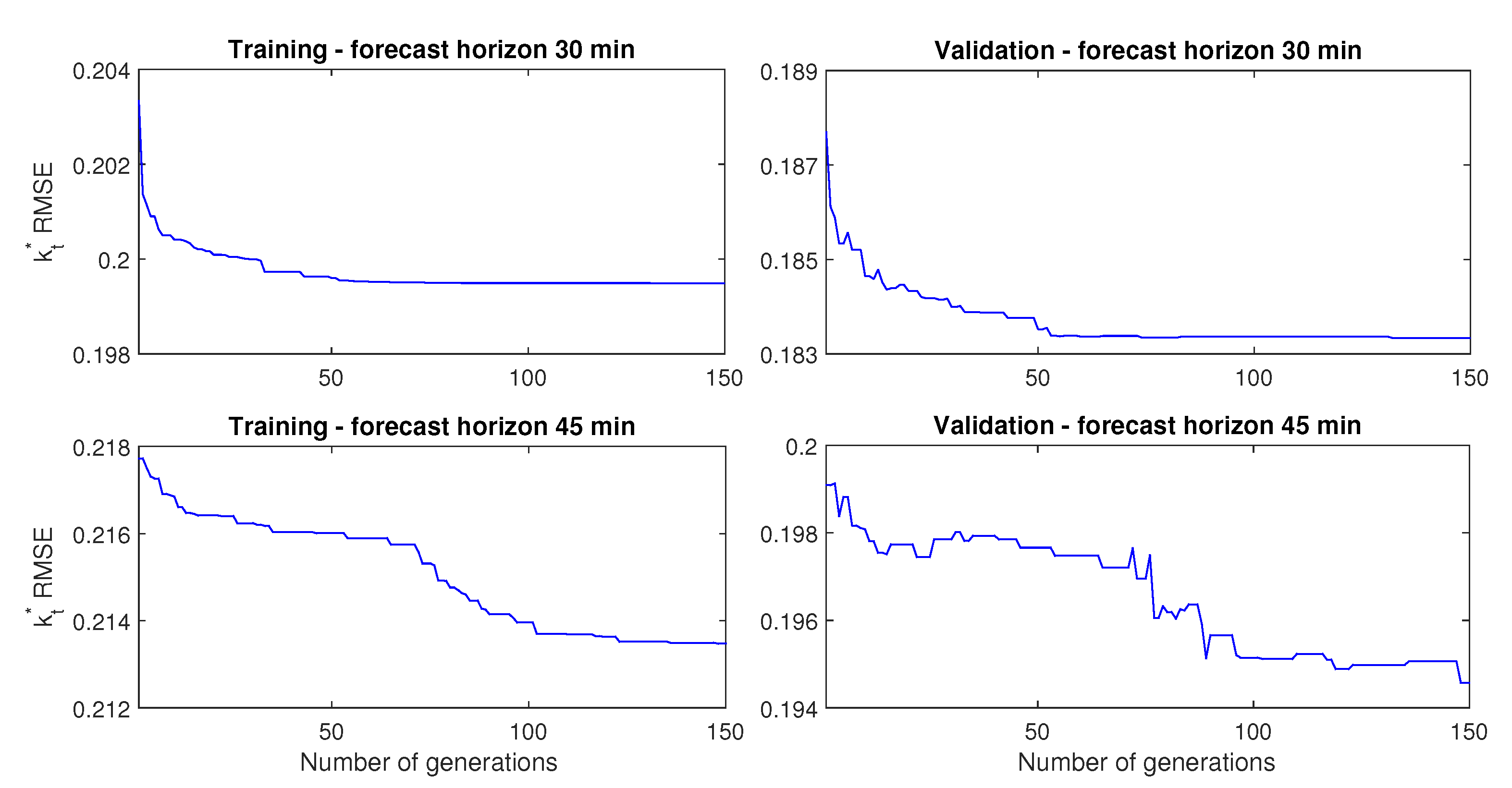
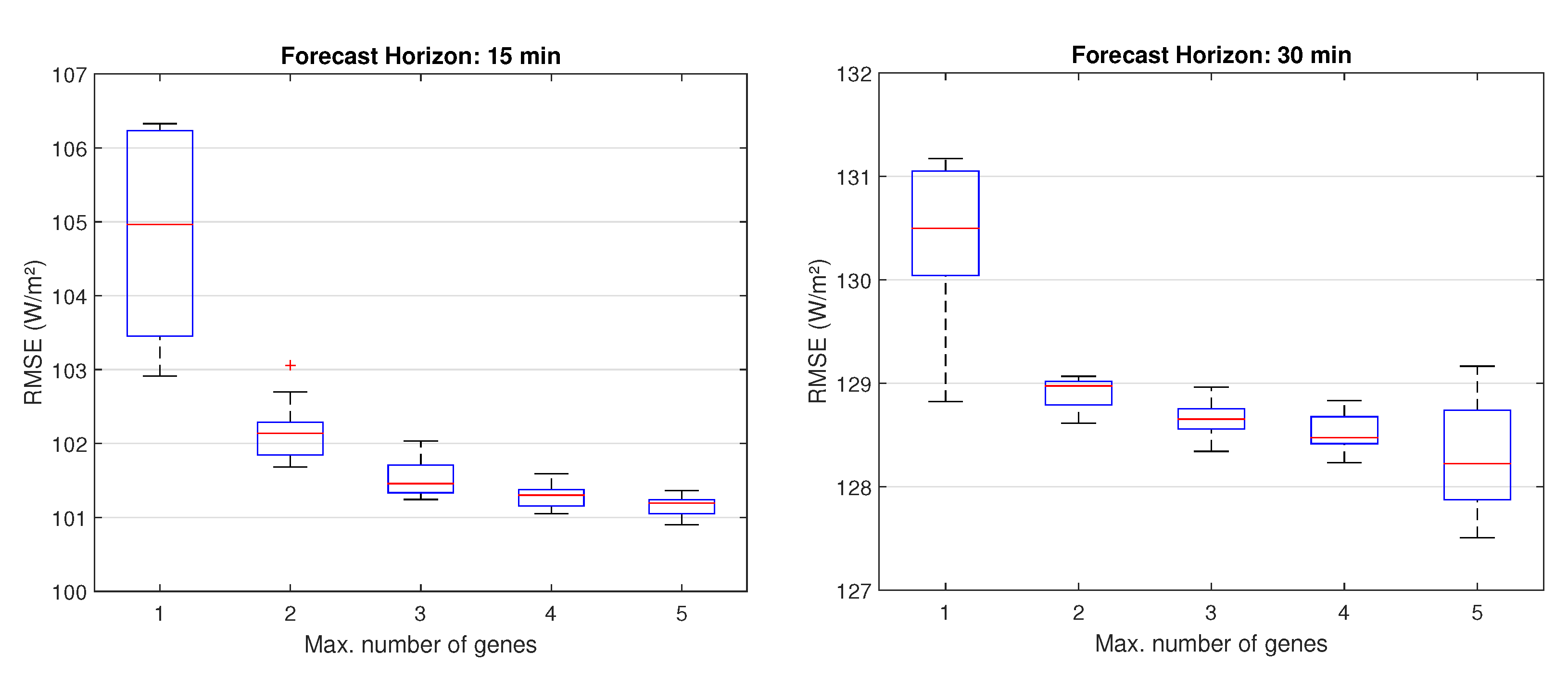
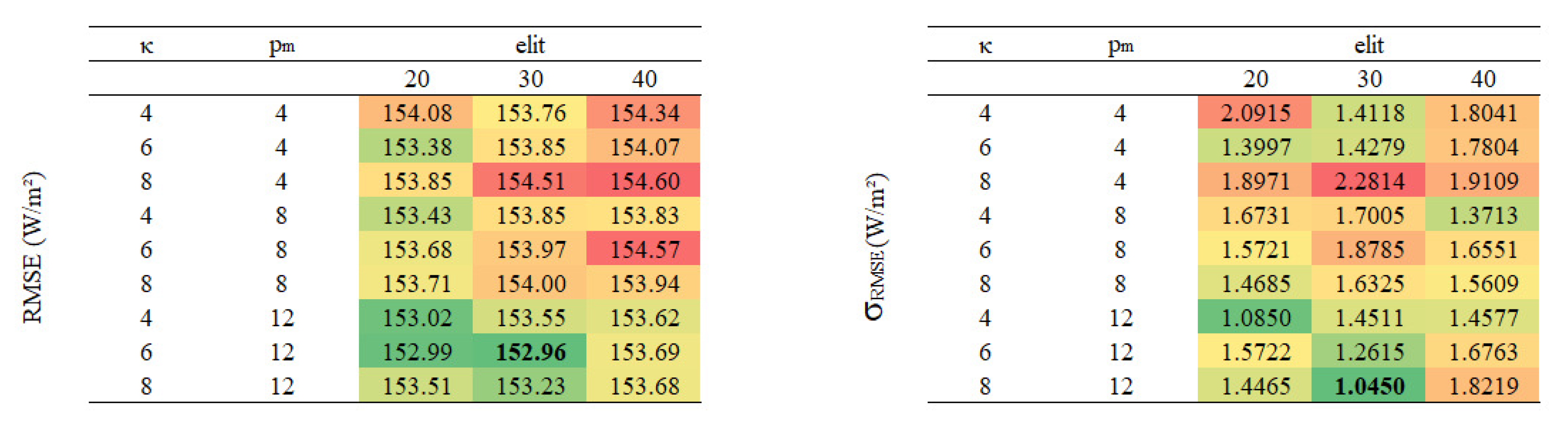
6.1. GP Tuning
6.2. Assessment of Exogenous Input
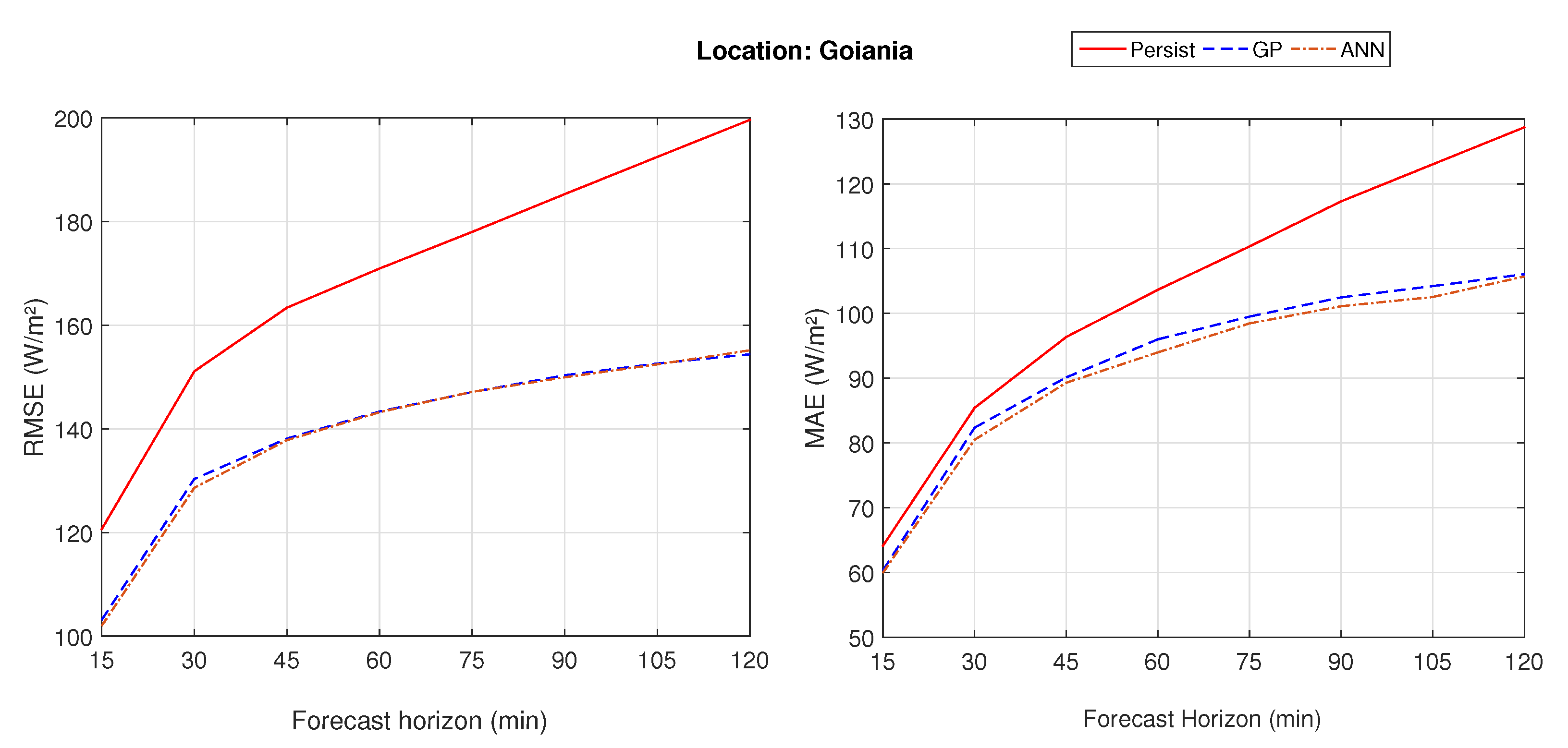
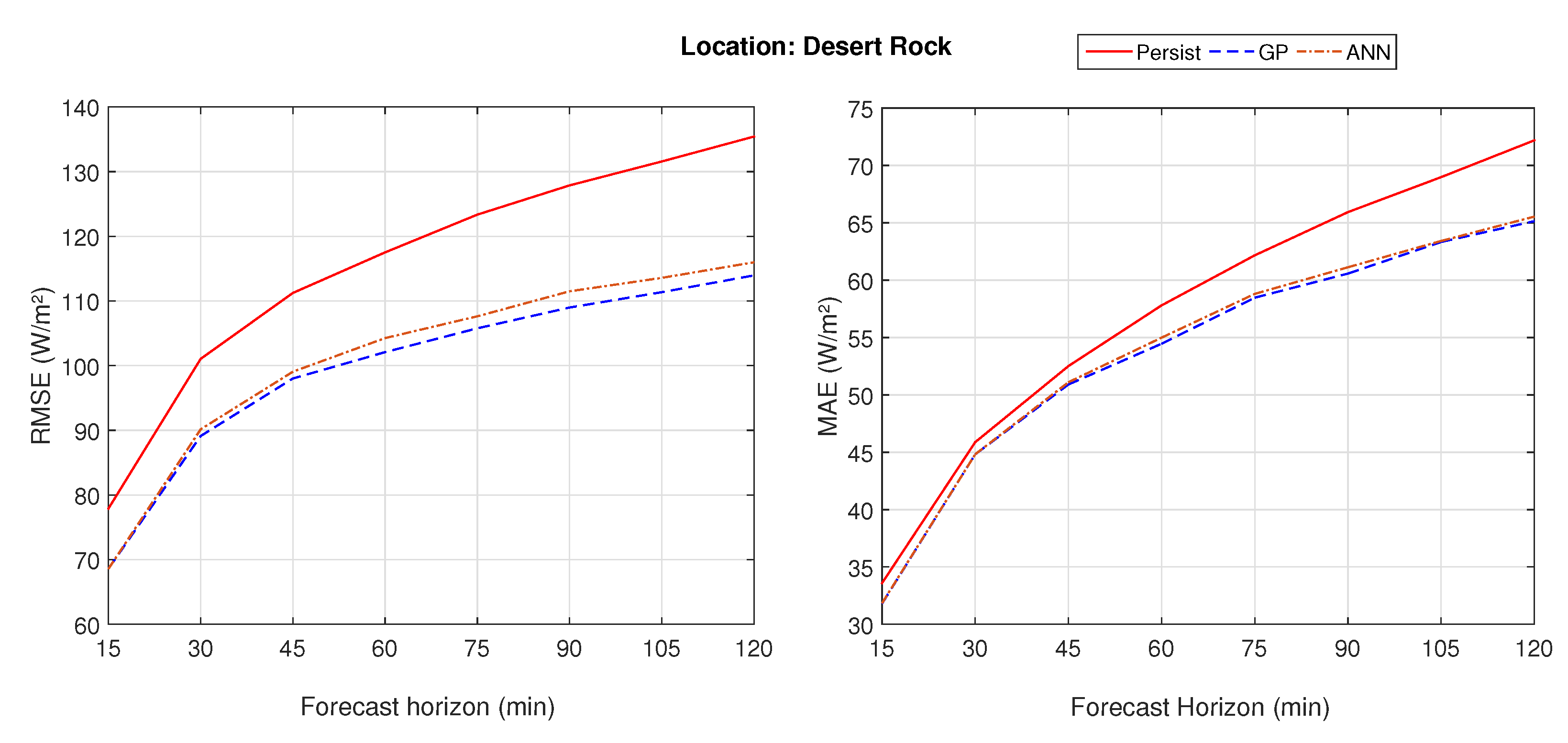
6.3. Specific Results
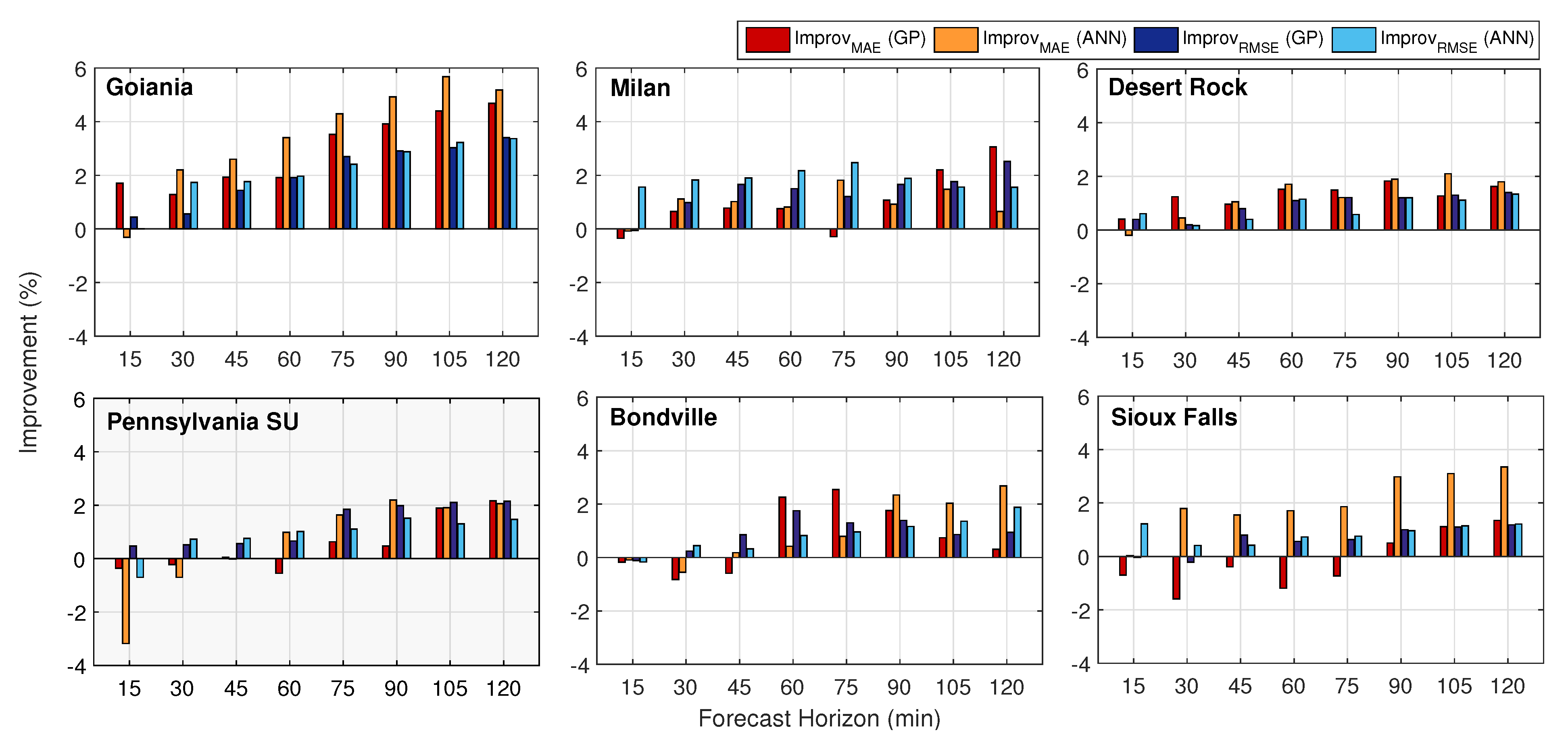
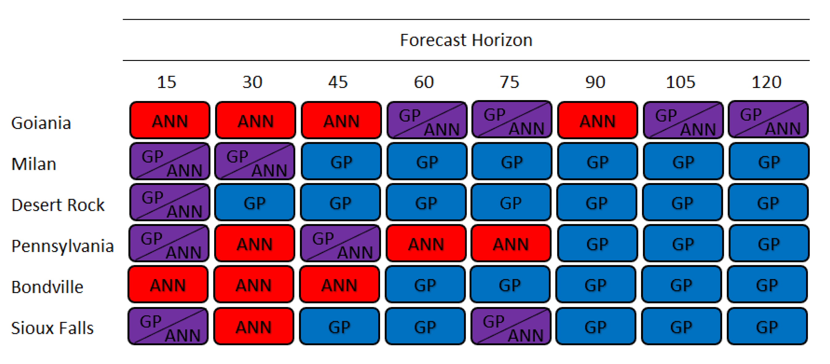
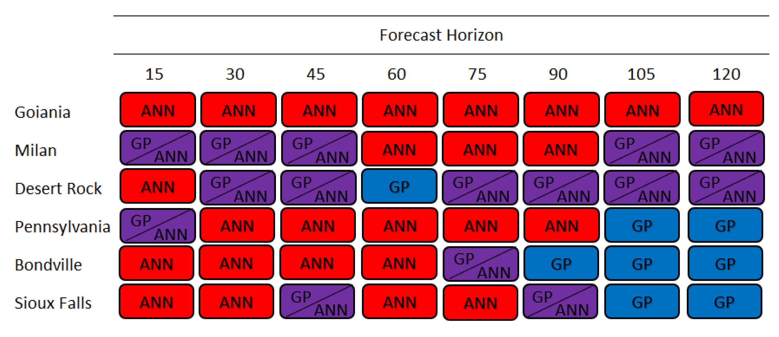
6.4. Generic Results
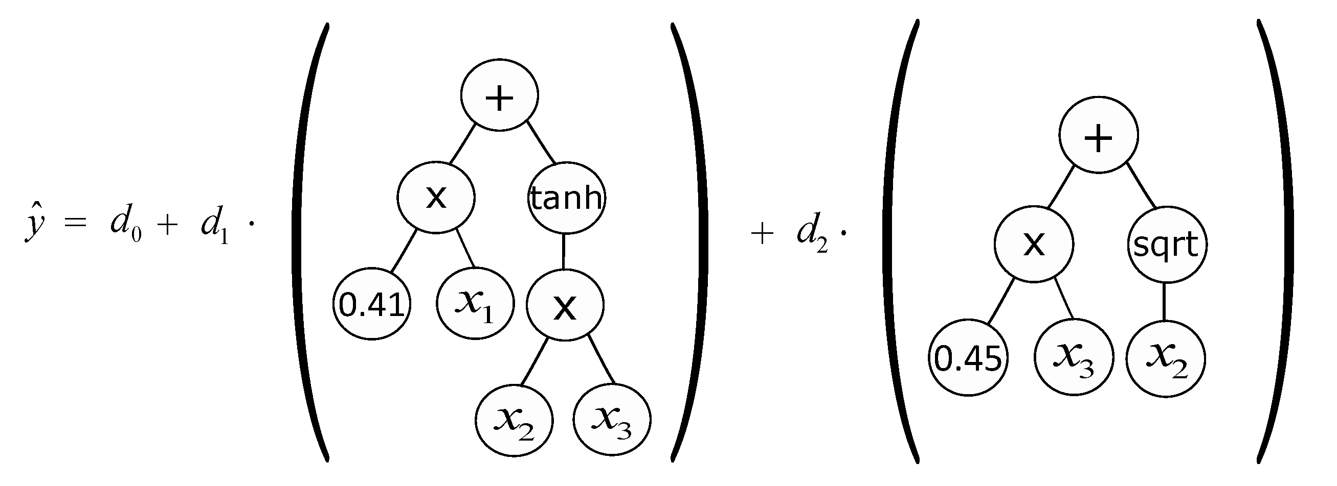
6.5. Regression Functions
6.6. Comparison with the State-of-the-Art
6.7. Machine Learning Algorithm Training Speed
7. Conclusions
Author Contributions
Funding
Acknowledgments
Conflicts of Interest
Abbreviations
| AM | Air mass |
| ANN | Artificial neural network |
| ARIMA | Autoregressive integrated moving average |
| EA | Evolutionary algorithms |
| GBR | Gradient boosted regression |
| GP | Genetic programming |
| IEA | International energy agency |
| kNN | k-Nearest neighbors |
| MAE | Mean absolute error |
| MGGP | Multigene genetic programming |
| ML | Machine learning |
| MLP | Multilayer perceptron |
| NOAA | National Oceanic and Atmospheric Administration |
| NWP | Numerical weather prediction |
| PSU | Pennsylvania State University |
| PV | Photovoltaic |
| RES | Renewable energy sources |
| RF | Random forest |
| RMSE | Root mean squared error |
| SURFRAD | Surface Radiation Network |
| SVM | Support vector machine |
Appendix A. Errors Obtained for Each Location, ML Algorithm and Forecast Horizon

| Haur. | Inei. | ||||||||||
|---|---|---|---|---|---|---|---|---|---|---|---|
| FH | Method | s | RMSE | MAE | s | RMSE | MAE | ||||
| 120.67 | 64.13 | 120.64 | 63.85 | ||||||||
| 14.51 | 103.16 | 0.28 | 60.32 | 0.29 | 14.29 | 103.40 | 0.37 | 60.09 | 0.62 | ||
| 15 | 15.46 | 102.02 | 0.27 | 59.97 | 0.44 | 15.08 | 102.45 | 0.37 | 60.19 | 0.45 | |
| 14.90 | 102.68 | 59.89 | 14.53 | 103.12 | 59.83 | ||||||
| 16.05 | 101.30 | 59.09 | 15.87 | 101.50 | 59.16 | ||||||
| 151.11 | 85.42 | 150.81 | 84.59 | ||||||||
| 13.75 | 130.34 | 0.52 | 82.36 | 0.61 | 13.56 | 130.36 | 0.29 | 82.31 | 0.37 | ||
| 30 | 14.87 | 128.64 | 0.59 | 80.49 | 0.72 | 14.49 | 128.95 | 0.39 | 81.02 | 0.90 | |
| 14.11 | 129.79 | 81.84 | 13.94 | 129.78 | 81.81 | ||||||
| 15.52 | 127.65 | 79.34 | 15.28 | 127.76 | 79.54 | ||||||
| 163.39 | 96.35 | 162.72 | 94.92 | ||||||||
| 15.46 | 138.13 | 0.31 | 90.12 | 0.36 | 14.93 | 138.43 | 0.44 | 90.94 | 0.28 | ||
| 45 | 15.65 | 137.82 | 0.37 | 89.29 | 0.40 | 15.03 | 138.26 | 0.50 | 89.86 | 0.65 | |
| 15.56 | 137.96 | 89.67 | 15.06 | 138.21 | 90.56 | ||||||
| 16.40 | 136.60 | 87.99 | 16.03 | 136.64 | 88.43 | ||||||
| 170.94 | 103.64 | 169.82 | 101.44 | ||||||||
| 16.13 | 143.36 | 0.40 | 96.00 | 0.42 | 15.92 | 142.78 | 0.26 | 95.69 | 0.46 | ||
| 60 | 16.21 | 143.22 | 0.75 | 93.98 | 1.21 | 15.77 | 143.04 | 0.50 | 94.52 | 0.69 | |
| 16.45 | 142.82 | 95.61 | 16.07 | 142.53 | 95.44 | ||||||
| 17.03 | 141.83 | 92.46 | 16.36 | 142.04 | 93.90 | ||||||
| 178.00 | 110.33 | 176.44 | 107.51 | ||||||||
| 17.36 | 147.11 | 0.45 | 99.50 | 0.41 | 16.70 | 146.98 | 0.25 | 99.56 | 0.41 | ||
| 75 | 17.34 | 147.15 | 0.66 | 98.45 | 0.79 | 16.42 | 147.47 | 0.52 | 98.81 | 0.50 | |
| 17.62 | 146.65 | 98.97 | 16.80 | 146.79 | 99.35 | ||||||
| 18.14 | 145.71 | 96.98 | 17.25 | 146.00 | 97.42 | ||||||
| 185.30 | 117.29 | 183.28 | 113.91 | ||||||||
| 18.86 | 150.35 | 0.40 | 102.47 | 0.45 | 18.18 | 149.96 | 0.40 | 102.16 | 0.63 | ||
| 90 | 19.08 | 149.95 | 0.43 | 101.11 | 0.68 | 18.03 | 150.23 | 0.28 | 101.49 | 0.88 | |
| 19.09 | 149.91 | 102.13 | 18.35 | 149.65 | 101.73 | ||||||
| 19.88 | 148.46 | 99.57 | 18.84 | 148.76 | 99.91 | ||||||
| 192.48 | 123.01 | 190.04 | 119.03 | ||||||||
| 20.71 | 152.61 | 0.35 | 104.21 | 0.53 | 19.91 | 152.21 | 0.36 | 104.13 | 0.35 | ||
| 105 | 20.79 | 152.45 | 0.50 | 102.52 | 0.56 | 19.45 | 153.09 | 0.81 | 103.82 | 1.30 | |
| 20.94 | 152.16 | 103.84 | 20.07 | 151.91 | 103.82 | ||||||
| 21.46 | 151.18 | 101.29 | 20.20 | 151.65 | 102.47 | ||||||
| 199.62 | 128.73 | 196.80 | 124.08 | ||||||||
| 22.65 | 154.40 | 0.27 | 106.04 | 0.32 | 21.58 | 154.33 | 0.37 | 105.85 | 0.49 | ||
| 120 | 22.27 | 155.17 | 0.92 | 105.71 | 1.01 | 21.12 | 155.24 | 0.77 | 106.49 | 1.00 | |
| 22.80 | 154.10 | 105.79 | 21.77 | 153.96 | 105.50 | ||||||
| 23.09 | 153.52 | 104.23 | 21.73 | 154.03 | 105.26 |
| Haur. | Inei. | ||||||||||
|---|---|---|---|---|---|---|---|---|---|---|---|
| FH | Method | s | RMSE | MAE | s | RMSE | MAE | ||||
| 76.02 | 37.43 | 75.97 | 37.33 | ||||||||
| 11.63 | 67.18 | 0.63 | 34.22 | 0.38 | 11.35 | 67.34 | 0.63 | 34.06 | 0.30 | ||
| 15 | 12.54 | 66.48 | 1.09 | 35.11 | 0.31 | 12.06 | 66.80 | 1.04 | 36.11 | 0.25 | |
| 12.23 | 66.72 | 33.84 | 11.95 | 66.89 | 33.69 | ||||||
| 14.81 | 64.76 | 34.11 | 14.01 | 65.32 | 34.18 | ||||||
| 99.41 | 51.12 | 99.29 | 50.80 | ||||||||
| 10.80 | 88.67 | 0.32 | 48.95 | 0.44 | 9.62 | 89.74 | 0.35 | 50.18 | 0.38 | ||
| 30 | 10.86 | 88.61 | 0.71 | 50.23 | 0.51 | 9.24 | 90.12 | 1.80 | 51.49 | 1.09 | |
| 11.12 | 88.36 | 48.65 | 10.12 | 89.24 | 49.73 | ||||||
| 12.62 | 86.87 | 48.90 | 11.82 | 87.55 | 48.92 | ||||||
| 110.31 | 59.34 | 110.12 | 58.76 | ||||||||
| 10.70 | 98.50 | 0.20 | 56.46 | 0.42 | 9.18 | 100.01 | 0.38 | 56.92 | 0.52 | ||
| 45 | 10.40 | 98.83 | 0.64 | 58.27 | 0.64 | 8.51 | 100.75 | 0.81 | 59.04 | 0.65 | |
| 10.87 | 98.32 | 56.25 | 9.46 | 99.70 | 56.63 | ||||||
| 12.01 | 97.06 | 56.94 | 11.02 | 97.99 | 57.17 | ||||||
| 120.03 | 66.08 | 119.82 | 65.28 | ||||||||
| 11.58 | 106.12 | 0.22 | 62.04 | 0.49 | 11.09 | 106.52 | 0.35 | 62.78 | 0.39 | ||
| 60 | 11.55 | 106.16 | 0.61 | 63.80 | 0.79 | 10.48 | 107.27 | 0.78 | 63.56 | 0.47 | |
| 11.83 | 105.83 | 61.75 | 11.52 | 106.02 | 62.70 | ||||||
| 12.87 | 104.58 | 62.50 | 11.91 | 105.54 | 61.69 | ||||||
| 128.66 | 72.05 | 128.54 | 71.04 | ||||||||
| 12.80 | 112.18 | 0.34 | 67.43 | 0.32 | 12.36 | 112.66 | 0.65 | 67.20 | 0.50 | ||
| 75 | 12.67 | 112.36 | 0.90 | 67.97 | 0.72 | 11.76 | 113.42 | 1.48 | 69.28 | 1.15 | |
| 12.44 | 112.65 | 67.22 | 12.50 | 112.47 | 67.03 | ||||||
| 13.94 | 110.72 | 66.63 | 13.35 | 111.38 | 67.63 | ||||||
| 136.10 | 77.66 | 136.15 | 76.32 | ||||||||
| 13.60 | 117.59 | 0.40 | 70.97 | 0.29 | 13.93 | 117.18 | 0.66 | 71.16 | 0.49 | ||
| 90 | 13.52 | 117.69 | 0.53 | 72.62 | 1.02 | 13.39 | 117.91 | 0.85 | 72.66 | 1.37 | |
| 13.87 | 117.22 | 70.78 | 14.35 | 116.61 | 70.86 | ||||||
| 14.79 | 115.97 | 71.25 | 15.08 | 115.62 | 70.74 | ||||||
| 142.26 | 82.92 | 142.50 | 81.48 | ||||||||
| 14.60 | 121.49 | 0.52 | 74.05 | 0.35 | 14.60 | 121.69 | 0.44 | 74.92 | 0.45 | ||
| 105 | 13.64 | 122.85 | 2.41 | 76.34 | 1.21 | 14.16 | 122.33 | 0.89 | 76.22 | 0.70 | |
| 14.77 | 121.26 | 73.85 | 14.77 | 121.46 | 74.71 | ||||||
| 15.45 | 120.29 | 74.41 | 15.71 | 120.11 | 74.56 | ||||||
| 147.60 | 87.74 | 148.21 | 86.14 | ||||||||
| 15.70 | 124.43 | 0.36 | 76.90 | 0.28 | 15.95 | 124.58 | 0.36 | 78.46 | 1.07 | ||
| 120 | 15.03 | 125.42 | 1.21 | 79.81 | 1.64 | 15.57 | 125.14 | 1.01 | 79.72 | 1.26 | |
| 15.83 | 124.24 | 76.73 | 16.13 | 124.30 | 78.28 | ||||||
| 16.25 | 123.61 | 78.47 | 16.97 | 123.06 | 78.15 |
| Haur. | Inei. | ||||||||||
|---|---|---|---|---|---|---|---|---|---|---|---|
| FH | Method | s | RMSE | MAE | s | RMSE | MAE | ||||
| 78.00 | 34.46 | 77.90 | 33.59 | ||||||||
| 11.96 | 68.68 | 0.14 | 31.64 | 0.18 | 11.94 | 68.60 | 0.23 | 31.81 | 0.23 | ||
| 15 | 11.98 | 68.66 | 0.25 | 31.85 | 0.56 | 11.98 | 68.57 | 0.29 | 31.84 | 0.51 | |
| 12.26 | 68.44 | 31.29 | 12.28 | 68.34 | 31.58 | ||||||
| 13.24 | 67.68 | 31.02 | 12.96 | 67.81 | 31.27 | ||||||
| 101.32 | 47.74 | 101.05 | 45.88 | ||||||||
| 11.45 | 89.72 | 0.57 | 45.24 | 0.41 | 11.80 | 89.12 | 0.09 | 44.82 | 0.45 | ||
| 30 | 10.74 | 90.44 | 0.71 | 44.93 | 0.43 | 10.78 | 90.16 | 0.53 | 44.83 | 0.37 | |
| 11.77 | 89.39 | 44.73 | 11.91 | 89.01 | 44.68 | ||||||
| 11.60 | 89.57 | 44.15 | 11.62 | 89.31 | 44.33 | ||||||
| 111.75 | 55.36 | 111.24 | 52.51 | ||||||||
| 12.09 | 98.24 | 0.28 | 50.87 | 0.35 | 11.89 | 98.02 | 1.41 | 50.91 | 1.08 | ||
| 45 | 10.98 | 99.49 | 0.46 | 50.94 | 1.00 | 10.95 | 99.06 | 0.22 | 51.10 | 0.67 | |
| 12.21 | 98.11 | 50.72 | 12.47 | 97.37 | 50.47 | ||||||
| 11.85 | 98.51 | 50.00 | 11.53 | 98.41 | 50.51 | ||||||
| 118.32 | 61.63 | 117.51 | 57.80 | ||||||||
| 13.05 | 102.88 | 0.32 | 55.24 | 0.38 | 13.13 | 102.09 | 0.15 | 54.46 | 0.16 | ||
| 60 | 11.81 | 104.34 | 1.21 | 56.51 | 1.01 | 11.28 | 104.26 | 0.29 | 54.99 | 0.47 | |
| 13.17 | 102.74 | 55.11 | 13.19 | 102.02 | 54.41 | ||||||
| 12.77 | 103.20 | 55.35 | 11.90 | 103.53 | 54.47 | ||||||
| 124.48 | 67.03 | 123.35 | 62.16 | ||||||||
| 14.46 | 106.48 | 0.11 | 59.12 | 0.10 | 14.25 | 105.77 | 0.11 | 58.47 | 0.34 | ||
| 75 | 13.34 | 107.88 | 0.33 | 59.70 | 1.50 | 12.74 | 107.63 | 0.47 | 58.80 | 0.60 | |
| 14.56 | 106.36 | 58.42 | 14.32 | 105.69 | 57.81 | ||||||
| 14.06 | 106.98 | 58.31 | 13.41 | 106.81 | 57.42 | ||||||
| 129.33 | 71.66 | 127.87 | 65.93 | ||||||||
| 15.18 | 109.70 | 0.20 | 61.55 | 0.36 | 14.77 | 108.98 | 0.15 | 60.57 | 0.24 | ||
| 90 | 13.87 | 111.40 | 0.76 | 61.60 | 0.91 | 12.81 | 111.50 | 0.80 | 61.12 | 0.65 | |
| 15.25 | 109.60 | 61.47 | 14.84 | 108.90 | 60.44 | ||||||
| 14.72 | 110.30 | 60.67 | 13.55 | 110.55 | 59.99 | ||||||
| 133.39 | 75.55 | 131.57 | 68.98 | ||||||||
| 16.06 | 111.97 | 0.14 | 63.15 | 0.22 | 15.36 | 111.36 | 0.15 | 63.13 | 0.27 | ||
| 105 | 14.22 | 114.42 | 0.70 | 63.20 | 0.89 | 13.68 | 113.57 | 0.39 | 63.42 | 0.60 | |
| 16.11 | 111.91 | 63.49 | 15.45 | 111.24 | 62.52 | ||||||
| 14.99 | 113.40 | 62.11 | 14.34 | 112.70 | 62.02 | ||||||
| 137.62 | 79.56 | 135.42 | 72.19 | ||||||||
| 16.83 | 114.46 | 0.20 | 66.09 | 0.25 | 15.85 | 113.96 | 0.15 | 65.14 | 0.29 | ||
| 120 | 15.60 | 116.15 | 0.56 | 65.59 | 0.52 | 14.36 | 115.98 | 0.42 | 65.54 | 1.16 | |
| 16.91 | 114.35 | 65.98 | 15.91 | 113.88 | 65.07 | ||||||
| 16.24 | 115.27 | 64.86 | 15.07 | 115.01 | 64.83 |
| Haur. | Inei. | ||||||||||
|---|---|---|---|---|---|---|---|---|---|---|---|
| FH | Method | s | RMSE | MAE | s | RMSE | MAE | ||||
| 94.43 | 51.76 | 94.37 | 51.49 | ||||||||
| 12.78 | 82.36 | 0.44 | 47.47 | 0.34 | 12.99 | 82.11 | 0.28 | 47.23 | 0.14 | ||
| 15 | 14.42 | 80.82 | 0.29 | 47.49 | 0.45 | 13.86 | 81.29 | 0.29 | 48.17 | 0.53 | |
| 13.31 | 81.86 | 47.10 | 13.39 | 81.73 | 46.92 | ||||||
| 14.98 | 80.28 | 47.00 | 14.49 | 80.69 | 47.57 | ||||||
| 118.31 | 68.46 | 118.13 | 67.85 | ||||||||
| 10.71 | 105.64 | 0.26 | 66.56 | 0.28 | 10.46 | 105.78 | 0.26 | 66.02 | 0.28 | ||
| 30 | 11.70 | 104.47 | 0.17 | 65.93 | 0.61 | 11.54 | 104.49 | 0.36 | 66.47 | 0.37 | |
| 11.05 | 105.23 | 66.23 | 10.77 | 105.40 | 65.78 | ||||||
| 12.34 | 103.72 | 65.28 | 12.29 | 103.62 | 65.66 | ||||||
| 131.38 | 78.48 | 131.05 | 77.51 | ||||||||
| 12.32 | 115.19 | 0.23 | 74.60 | 0.40 | 11.85 | 115.52 | 0.21 | 74.30 | 0.29 | ||
| 45 | 13.07 | 114.21 | 0.28 | 74.80 | 0.63 | 12.71 | 114.39 | 0.23 | 74.52 | 0.45 | |
| 12.61 | 114.82 | 74.26 | 12.06 | 115.24 | 74.01 | ||||||
| 13.76 | 113.30 | 74.07 | 13.44 | 113.44 | 73.69 | ||||||
| 138.63 | 84.75 | 138.19 | 83.45 | ||||||||
| 12.54 | 121.25 | 0.06 | 79.96 | 0.17 | 12.17 | 121.37 | 0.29 | 80.29 | 0.31 | ||
| 60 | 13.11 | 120.45 | 0.36 | 79.94 | 0.87 | 12.67 | 120.69 | 0.41 | 80.03 | 0.72 | |
| 12.68 | 121.06 | 79.78 | 12.39 | 121.06 | 80.00 | ||||||
| 13.68 | 119.66 | 79.28 | 13.42 | 119.64 | 79.17 | ||||||
| 144.19 | 90.43 | 143.68 | 88.84 | ||||||||
| 12.65 | 125.95 | 0.11 | 84.92 | 0.21 | 12.40 | 125.86 | 0.86 | 84.80 | 0.97 | ||
| 75 | 12.88 | 125.62 | 0.48 | 84.87 | 0.98 | 12.57 | 125.63 | 0.42 | 84.71 | 0.40 | |
| 12.86 | 125.65 | 84.71 | 12.77 | 125.33 | 84.45 | ||||||
| 13.57 | 124.63 | 84.10 | 13.27 | 124.61 | 83.81 | ||||||
| 150.58 | 96.09 | 150.03 | 94.27 | ||||||||
| 13.34 | 130.50 | 0.36 | 89.32 | 0.20 | 13.63 | 129.59 | 0.29 | 89.07 | 0.37 | ||
| 90 | 13.27 | 130.59 | 0.61 | 89.37 | 0.98 | 13.06 | 130.43 | 0.50 | 89.50 | 0.68 | |
| 13.52 | 130.23 | 89.09 | 13.77 | 129.37 | 88.89 | ||||||
| 14.13 | 129.30 | 88.42 | 13.89 | 129.19 | 88.57 | ||||||
| 156.99 | 101.08 | 156.42 | 99.04 | ||||||||
| 14.97 | 133.48 | 0.13 | 92.24 | 0.21 | 14.69 | 133.44 | 0.38 | 92.10 | 0.43 | ||
| 105 | 14.38 | 134.42 | 0.23 | 92.99 | 0.94 | 13.85 | 134.75 | 0.45 | 93.37 | 0.53 | |
| 15.14 | 133.22 | 92.13 | 14.90 | 133.11 | 91.71 | ||||||
| 15.08 | 133.31 | 92.23 | 14.67 | 133.46 | 92.44 | ||||||
| 164.37 | 106.50 | 163.82 | 104.31 | ||||||||
| 16.23 | 137.70 | 0.21 | 95.99 | 0.15 | 16.21 | 137.27 | 0.22 | 95.95 | 0.22 | ||
| 120 | 15.50 | 138.90 | 0.82 | 97.39 | 0.93 | 15.08 | 139.12 | 0.74 | 97.70 | 1.02 | |
| 16.36 | 137.48 | 95.85 | 16.37 | 137.00 | 95.73 | ||||||
| 16.25 | 137.66 | 96.57 | 15.91 | 137.75 | 96.73 |
| Haur. | Inei. | ||||||||||
|---|---|---|---|---|---|---|---|---|---|---|---|
| FH | Method | s | RMSE | MAE | s | RMSE | MAE | ||||
| 81.28 | 43.45 | 81.20 | 43.01 | ||||||||
| 10.43 | 72.81 | 0.77 | 41.51 | 0.35 | 10.85 | 72.39 | 0.41 | 41.05 | 0.15 | ||
| 15 | 11.74 | 71.74 | 0.49 | 40.87 | 0.59 | 11.10 | 72.18 | 0.41 | 41.26 | 0.34 | |
| 11.31 | 72.09 | 41.05 | 11.30 | 72.02 | 40.84 | ||||||
| 12.71 | 70.95 | 40.22 | 11.92 | 71.52 | 40.71 | ||||||
| 101.49 | 57.67 | 101.25 | 56.79 | ||||||||
| 9.97 | 91.37 | 0.47 | 56.08 | 0.56 | 10.23 | 90.89 | 0.28 | 56.38 | 0.29 | ||
| 30 | 10.16 | 91.18 | 0.48 | 55.92 | 0.73 | 9.57 | 91.56 | 0.29 | 56.50 | 0.21 | |
| 10.35 | 90.98 | 55.75 | 10.52 | 90.61 | 56.15 | ||||||
| 10.94 | 90.38 | 55.32 | 10.41 | 90.71 | 55.78 | ||||||
| 113.22 | 66.80 | 112.82 | 65.39 | ||||||||
| 9.83 | 102.09 | 0.52 | 64.38 | 0.48 | 10.28 | 101.22 | 0.42 | 64.37 | 0.53 | ||
| 45 | 10.61 | 101.20 | 0.32 | 63.27 | 0.68 | 9.82 | 101.74 | 0.89 | 64.49 | 1.34 | |
| 10.26 | 101.60 | 63.92 | 10.56 | 100.91 | 64.15 | ||||||
| 11.37 | 100.35 | 62.57 | 10.74 | 100.71 | 63.72 | ||||||
| 121.55 | 73.53 | 120.99 | 71.70 | ||||||||
| 11.65 | 107.39 | 0.35 | 69.37 | 0.42 | 11.16 | 107.48 | 0.46 | 69.76 | 0.79 | ||
| 60 | 11.38 | 107.73 | 0.33 | 69.37 | 0.48 | 10.72 | 108.02 | 0.37 | 69.98 | 0.54 | |
| 12.06 | 106.90 | 68.94 | 11.58 | 106.97 | 69.30 | ||||||
| 12.15 | 106.79 | 68.64 | 11.53 | 107.04 | 69.15 | ||||||
| 127.95 | 79.19 | 127.21 | 77.04 | ||||||||
| 12.01 | 112.58 | 0.11 | 73.78 | 0.20 | 11.19 | 112.97 | 0.30 | 73.98 | 0.32 | ||
| 75 | 11.52 | 113.21 | 0.49 | 74.30 | 0.83 | 10.62 | 113.71 | 1.01 | 74.83 | 1.01 | |
| 12.22 | 112.31 | 73.47 | 11.43 | 112.67 | 73.70 | ||||||
| 12.29 | 112.23 | 73.56 | 11.62 | 112.43 | 73.77 | ||||||
| 134.49 | 84.73 | 133.56 | 82.22 | ||||||||
| 13.22 | 116.71 | 0.19 | 77.69 | 0.21 | 12.15 | 117.33 | 0.22 | 78.67 | 0.28 | ||
| 90 | 12.24 | 118.03 | 0.51 | 78.32 | 0.74 | 11.40 | 118.33 | 0.71 | 78.93 | 0.48 | |
| 13.37 | 116.51 | 77.49 | 12.29 | 117.14 | 78.49 | ||||||
| 12.99 | 117.02 | 77.53 | 12.44 | 116.94 | 77.77 | ||||||
| 140.34 | 89.83 | 139.23 | 86.79 | ||||||||
| 13.52 | 121.37 | 0.32 | 81.88 | 0.39 | 12.21 | 122.23 | 0.22 | 82.32 | 0.45 | ||
| 105 | 12.56 | 122.71 | 0.69 | 82.06 | 0.52 | 11.90 | 122.66 | 0.55 | 82.70 | 0.45 | |
| 13.87 | 120.87 | 81.01 | 12.43 | 121.93 | 82.10 | ||||||
| 13.40 | 121.53 | 81.18 | 12.96 | 121.19 | 81.49 | ||||||
| 145.88 | 95.01 | 144.58 | 91.41 | ||||||||
| 14.42 | 124.84 | 0.35 | 85.95 | 0.31 | 12.96 | 125.85 | 0.72 | 86.30 | 0.55 | ||
| 120 | 13.31 | 126.46 | 0.77 | 86.47 | 1.35 | 12.54 | 126.46 | 0.55 | 86.82 | 0.76 | |
| 14.59 | 124.59 | 85.07 | 13.25 | 125.42 | 85.79 | ||||||
| 14.45 | 124.80 | 85.30 | 13.59 | 124.93 | 85.66 |
| Haur. | Inei. | ||||||||||
|---|---|---|---|---|---|---|---|---|---|---|---|
| FH | Method | s | RMSE | MAE | s | RMSE | MAE | ||||
| 75.47 | 40.51 | 75.40 | 40.06 | ||||||||
| 10.09 | 67.85 | 0.30 | 38.17 | 0.24 | 10.13 | 67.76 | 0.23 | 37.82 | 0.19 | ||
| 15 | 12.25 | 66.23 | 0.20 | 38.02 | 0.18 | 11.70 | 66.58 | 1.04 | 38.41 | 0.25 | |
| 10.46 | 67.58 | 37.91 | 10.32 | 67.61 | 37.70 | ||||||
| 13.04 | 65.63 | 37.55 | 12.76 | 65.78 | 37.78 | ||||||
| 95.39 | 54.00 | 95.22 | 53.11 | ||||||||
| 9.22 | 86.60 | 0.10 | 52.86 | 0.17 | 8.71 | 86.93 | 0.28 | 52.97 | 0.25 | ||
| 30 | 9.51 | 86.32 | 0.45 | 53.15 | 0.51 | 9.17 | 86.49 | 0.26 | 52.82 | 0.42 | |
| 9.31 | 86.51 | 52.77 | 9.20 | 86.46 | 52.77 | ||||||
| 10.38 | 85.49 | 52.56 | 9.95 | 85.75 | 52.27 | ||||||
| 107.46 | 62.87 | 107.17 | 61.44 | ||||||||
| 9.56 | 97.18 | 0.21 | 60.86 | 0.42 | 9.72 | 96.75 | 0.09 | 60.69 | 0.42 | ||
| 45 | 9.84 | 96.89 | 0.51 | 61.69 | 0.69 | 9.57 | 96.91 | 0.30 | 61.03 | 0.48 | |
| 9.79 | 96.94 | 60.61 | 10.00 | 96.45 | 60.46 | ||||||
| 10.62 | 96.05 | 61.13 | 10.23 | 96.20 | 60.52 | ||||||
| 116.51 | 69.81 | 116.12 | 67.95 | ||||||||
| 10.59 | 104.17 | 0.11 | 66.92 | 0.23 | 10.42 | 104.03 | 0.17 | 67.09 | 0.30 | ||
| 60 | 10.16 | 104.68 | 0.38 | 67.47 | 0.33 | 10.20 | 104.27 | 0.45 | 67.05 | 0.46 | |
| 10.72 | 104.02 | 66.80 | 10.52 | 103.90 | 66.96 | ||||||
| 10.98 | 103.72 | 66.74 | 10.98 | 103.37 | 66.39 | ||||||
| 123.64 | 75.45 | 123.21 | 73.35 | ||||||||
| 11.18 | 109.82 | 0.20 | 71.76 | 0.33 | 11.01 | 109.64 | 0.14 | 71.93 | 0.39 | ||
| 75 | 10.92 | 110.14 | 0.58 | 72.21 | 0.86 | 10.76 | 109.95 | 0.33 | 71.58 | 0.67 | |
| 11.37 | 109.58 | 71.56 | 11.18 | 109.43 | 71.73 | ||||||
| 11.75 | 109.11 | 71.49 | 11.51 | 109.03 | 70.92 | ||||||
| 130.98 | 81.05 | 130.57 | 78.71 | ||||||||
| 12.47 | 114.65 | 0.19 | 75.83 | 0.15 | 12.31 | 114.49 | 0.11 | 75.46 | 0.35 | ||
| 90 | 11.84 | 115.48 | 0.42 | 76.45 | 1.00 | 11.60 | 115.42 | 0.27 | 76.37 | 0.76 | |
| 12.65 | 114.42 | 75.62 | 12.42 | 114.35 | 75.33 | ||||||
| 12.71 | 114.34 | 75.66 | 12.43 | 114.34 | 75.59 | ||||||
| 138.49 | 86.65 | 138.10 | 83.89 | ||||||||
| 13.92 | 119.20 | 0.15 | 79.62 | 0.34 | 13.70 | 119.18 | 0.25 | 79.31 | 0.21 | ||
| 105 | 12.90 | 120.62 | 0.20 | 80.50 | 0.59 | 12.99 | 120.17 | 0.50 | 80.39 | 0.79 | |
| 14.12 | 118.94 | 79.41 | 13.94 | 118.85 | 79.10 | ||||||
| 13.81 | 119.36 | 79.65 | 13.88 | 118.94 | 79.52 | ||||||
| 143.72 | 91.37 | 143.38 | 88.30 | ||||||||
| 14.59 | 122.75 | 0.32 | 82.76 | 0.20 | 13.98 | 123.34 | 0.92 | 83.06 | 1.03 | ||
| 120 | 13.71 | 124.02 | 0.63 | 84.05 | 0.48 | 13.34 | 124.26 | 0.60 | 83.99 | 0.81 | |
| 14.76 | 122.50 | 82.52 | 14.34 | 122.82 | 82.70 | ||||||
| 14.52 | 122.85 | 83.29 | 14.23 | 122.97 | 83.11 |
References
- Liang, H.; Tamang, A.K.; Zhuang, W.; Shen, X.S. Stochastic information management in smart grid. IEEE Commun. Surv. Tutor. 2014, 16, 1746–1770. [Google Scholar] [CrossRef]
- Bagheri, A.; Zhao, C.; Qiu, F.; Wang, J. Resilient transmission hardening planning in a high renewable penetration era. IEEE Trans. Power Syst. 2019, 34, 873–882. [Google Scholar] [CrossRef]
- Lahon, R.; Gupta, C.P. Energy management of cooperative microgrids with high-penetration renewables. IET Renew. Power Gener. 2018, 12, 680–690. [Google Scholar] [CrossRef]
- Lauret, P.; Perez, R.; Aguiar, L.M.; Tapachès, E.; Diagne, H.M.; David, M. Characterization of the intraday variability regime of solar irradiation of climatically distinct locations. Sol. Energy 2016, 125, 99–110. [Google Scholar] [CrossRef]
- Shahriari, M.; Blumsack, S. Scaling of wind energy variability over space and time. Appl. Energy 2017, 195, 572–585. [Google Scholar] [CrossRef]
- Bakirtzis, E.A.; Biskas, P.N. Multiple time resolution stochastic scheduling for systems with high renewable penetration. IEEE Trans. Power Syst. 2017, 32, 1030–1040. [Google Scholar] [CrossRef]
- Du, E.; Zhang, N.; Hodge, B.; Wang, Q.; Lu, Z.; Kang, C.; Kroposki, B.; Xia, Q. Operation of a high renewable penetrated power system with csp plants: A look-ahead stochastic unit commitment model. IEEE Trans. Power Syst. 2019, 34, 140–151. [Google Scholar] [CrossRef]
- Pelland, S.; Remund, J.; Keissl, J.; Oozeki, T.; Brabandere, K.D. Photovoltaic and Solar Forecasting: State of the Art; Tech. rep.; International Energy Agency: Paris, France, 2013. [Google Scholar]
- Yang, D.; Kleissl, J.; Gueymard, C.A.; Pedro, H.T.; Coimbra, C.F. History and trends in solar irradiance and pv power forecasting: A preliminary assessment and review using text mining. Sol. Energy 2018, 168, 60–101. [Google Scholar] [CrossRef]
- Diagne, M.; David, M.; Lauret, P.; Boland, J.; Schmutz, N. Review of solar irradiance forecasting methods and a proposition for small-scale insular grids. Renew. Sustain. Energy Rev. 2013, 27, 65–76. [Google Scholar] [CrossRef]
- Voyant, C.; Notton, G.; Kalogirou, S.; Nivet, M.-L.; Paoli, C.; Motte, F.; Fouilloy, A. Machine learning methods for solar radiation forecasting: A review. Renew. Energy 2017, 105, 569–582. [Google Scholar] [CrossRef]
- Sperati, S.; Alessandrini, S.; Pinson, P.; Kariniotakis, G. The “weather intelligence for renewable energies” benchmarking exercise on short-term forecasting of wind and solar power generation. Energies 2015, 8, 9594–9619. [Google Scholar] [CrossRef]
- Li, J.; Ward, J.K.; Tong, J.; Collins, L.; Platt, G. Machine learning for solar irradiance forecasting of photovoltaic system. Renew. Energy 2016, 90, 542–553. [Google Scholar] [CrossRef]
- Pedro, H.T.; Coimbra, C.F. Short-term irradiance forecastability for various solar micro-climates. Sol. Energy 2015, 122, 587–602. [Google Scholar] [CrossRef]
- Benali, L.; Notton, G.; Fouilloy, A.; Voyant, C.; Dizene, R. Solar radiation forecasting using artificial neural network and random forest methods: Application to normal beam, horizontal diffuse and global components. Renew. Energy 2019, 132, 871–884. [Google Scholar] [CrossRef]
- Persson, C.; Bacher, P.; Shiga, T.; Madsen, H. Multi-site solar power forecasting using gradient boosted regression trees. Solar Energy 2017, 150, 423–436. [Google Scholar] [CrossRef]
- Rana, M.; Koprinska, I.; Agelidis, V.G. Univariate and multivariate methods for very short-term solar photovoltaic power forecasting. Energy Convers. Manag. 2016, 121, 380–390. [Google Scholar] [CrossRef]
- Zeng, J.; Qiao, W. Short-term solar power prediction using a support vector machine. Renew. Energy 2013, 52, 118–127. [Google Scholar] [CrossRef]
- Dolara, A.; Grimaccia, F.; Leva, S.; Mussetta, M.; Ogliari, E. A Physical Hybrid Artificial Neural Network for Short Term Forecasting of PV Plant Power Output. Energies 2015, 8, 1138–1153. [Google Scholar] [CrossRef]
- Nobre, A.M.; Severiano, C.A.; Karthik, S.; Kubis, M.; Zhao, L.; Martins, F.R.; Pereira, E.B.; Rüther, R.; Reindl, T. Pv power conversion and short-term forecasting in a tropical, densely-built environment in Singapore. Renew. Energy 2016, 94, 496–509. [Google Scholar] [CrossRef]
- Reikard, G.; Hansen, C. Forecasting solar irradiance at short horizons: Frequency and time domain models. Renew. Energy 2019, 135, 1270–1290. [Google Scholar] [CrossRef]
- Yang, H.; Kurtz, B.; Nguyen, D.; Urquhart, B.; Chow, C.W.; Ghonima, M.; Kleissl, J. Solar irradiance forecasting using a ground-based sky imager developed at uc san diego. Sol. Energy 2014, 103, 502–524. [Google Scholar] [CrossRef]
- Chow, C.W.; Urquhart, B.; Lave, M.; Dominguez, A.; Kleissl, J.; Shields, J.; Washom, B. Intra-hour forecasting with a total sky imager at the uc san diego solar energy testbed. Sol. Energy 2011, 85, 2881–2893. [Google Scholar] [CrossRef]
- Dong, Z.; Yang, D.; Reindl, T.; Walsh, W.M. Satellite image analysis and a hybrid esss/ann model to forecast solar irradiance in the tropics. Energy Convers. Manag. 2014, 79, 66–73. [Google Scholar] [CrossRef]
- Bessa, R.J.; Trindade, A.; Miranda, V. Spatial-temporal solar power forecasting for smart grids. IEEE Trans. Ind. Informat. 2015, 11, 232–241. [Google Scholar] [CrossRef]
- Gutierrez-Corea, F.-V.; Manso-Callejo, M.-A.; Moreno-Regidor, M.-P.; Manrique-Sancho, M.-T. Forecasting short-term solar irradiance based on artificial neural networks and data from neighboring meteorological stations. Sol. Energy 2016, 134, 119–131. [Google Scholar] [CrossRef]
- Aguiar, L.M.; Pereira, B.; Lauret, P.; Díaz, F.; David, M. Combining solar irradiance measurements, satellite-derived data and a numerical weather prediction model to improve intra-day solar forecasting. Renew. Energy 2016, 97, 599–610. [Google Scholar] [CrossRef]
- Solar lab EMC/UFG. Federal University of Goias. Brazil. Available online: https://sites.google.com/site/sfvemcufg/ (accessed on 4 June 2020).
- SoDa. Solar Energy Services for Professionals. France. 2017. Available online: http://www.soda-pro.com/home;jsessionid=B032D33B0AD3460B741E14E41CC46BE2 (accessed on 4 June 2020).
- SolarTech Lab. Politecnico di Milano. Italy. Available online: http://www.solartech.polimi.it/ (accessed on 4 June 2020).
- De Paiva, G.M.; Pimentel, S.P.; Leva, S.; Mussetta, M. Intelligent approach to improve genetic programming based intra-day solar forecasting models. In Proceedings of the 2018 IEEE Congress on Evolutionary Computation (CEC), Rio de Janeiro, Brazil, 8–13 July 2018; pp. 1–8. [Google Scholar] [CrossRef]
- Reno, M.J.; Hansen, C.W.; Stein, J.S. Global Horizontal Irradiance Clear Sky Models: Implementation and Analysis; Tech. rep.; Sandia National Laboratories: Albuquerque, NM, USA, 2012.
- Duffie, J.A.; Beckman, W.A. Solar Engineering of Thermal Processes; John Wiley & Sons, Inc.: Hoboken, NJ, USA, 2013. [Google Scholar]
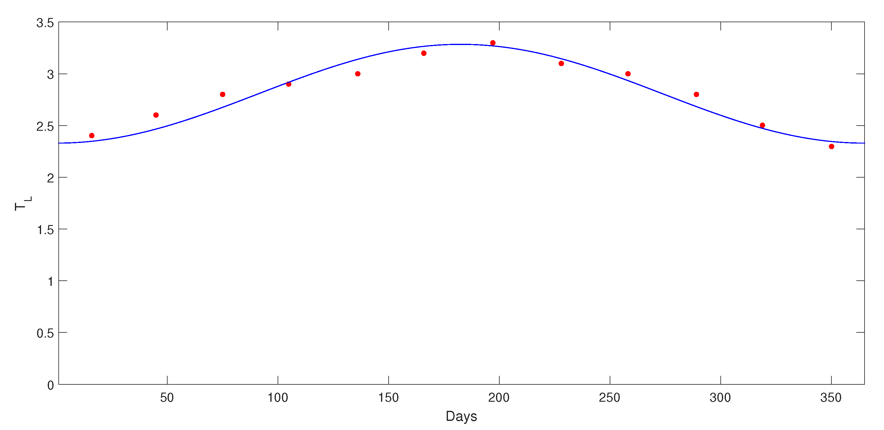
- Ineichen, P.; Perez, R. A new airmass independent formulation for the linke turbidity coefficient. Sol. Energy 2002, 73, 151–157. [Google Scholar] [CrossRef]
- Ineichen, P. Comparison of eight clear sky broadband models against 16 independent data banks. Sol. Energy 2006, 80, 468–478. [Google Scholar] [CrossRef]
- Engerer, N.; Mills, F. Kpv: A clear-sky index for photovoltaics. Sol. Energy 2014, 105, 679–693. [Google Scholar] [CrossRef]
- Koza, J.R. Genetic Programming: On the Programming of Computers by Means of Natural Selection; MIT Press: Cambridge, MA, USA, 1992. [Google Scholar]
- Brownlee, J. Clever Algorithms: Nature-Inspired Programming Recipes, 1st ed.; Lulu Press, Inc.: Morrisville, NC, USA, 2011. [Google Scholar]
- Lee, Y.-S.; Tong, L.-I. Forecasting time series using a methodology based on autoregressive integrated moving average and genetic programming. Knowl.-Based Syst. 2011, 24, 66–72. [Google Scholar] [CrossRef]
- Garg, A.; Sriram, S.; Tai, K. Empirical analysis of model selection criteria for genetic programming in modeling of time series system. In Proceedings of the 2013 IEEE Conference on Computational Intelligence for Financial Engineering Economics (CIFEr), Singapore, Singapore, 16–19 April 2013; IEEE: Piscataway, NJ, USA; pp. 90–94. [Google Scholar] [CrossRef]
- Mehr, A.D.; Kahya, E.; Olyaie, E. Streamflow prediction using linear genetic programming in comparison with a neuro-wavelet technique. J. Hydrol. 2013, 505, 240–249. [Google Scholar] [CrossRef]
- Ghorbani, M.A.; Khatibi, R.; Mehr, A.D.; Asadi, H. Chaos-based multigene genetic programming: A new hybrid strategy for river flow forecasting. J. Hydrol. 2018, 562, 455–467. [Google Scholar] [CrossRef]
- Mehr, A.D.; Jabarnejad, M.; Nourani, V. Pareto-optimal mpsa-mggp: A new gene-annealing model for monthly rainfall forecasting. J. Hydrol. 2019, 571, 406–415. [Google Scholar] [CrossRef]
- Russo, M.; Leotta, G.; Pugliatti, P.; Gigliucci, G. Genetic programming for photovoltaic plant output forecasting. Sol. Energy 2014, 105, 264–273. [Google Scholar] [CrossRef]
- Pan, I.; Pandey, D.S.; Das, S. Global solar irradiation prediction using a multi-gene genetic programming approach. J. Renew. Sustain. Energy 2013, 5, 063129. [Google Scholar] [CrossRef]
- Ghimire, S.; Deo, R.C.; Downs, N.J.; Raj, N. Global solar radiation prediction by ann integrated with european centre for medium range weather forecast fields in solar rich cities of queensland australia. J. Clean. Prod. 2019, 216, 288–310. [Google Scholar] [CrossRef]
- Searson, D.; Leahy, D.; Willis, M. GPTIPS: An open source genetic programming toolbox for multigene symbolic regression. In Proceedings of the International Multiconference of Engineers and Computer Scientists, Hong Kong, 17–19 March 2010; IAENG: Hong Kong, 2010; pp. 77–80. [Google Scholar]
- Leva, S.; Dolara, A.; Grimaccia, F.; Mussetta, M.; Ogliari, E. Analysis and validation of 24 hours ahead neural network forecasting of photovoltaic output power. Math. Comput. Simul. 2017, 131, 88–100. [Google Scholar] [CrossRef]
- Eiben, A.; Smit, S. Parameter tuning for configuring and analyzing evolutionary algorithms. Swarm Evol. Comput. 2011, 1, 19–31. [Google Scholar] [CrossRef]
- Lima, E.B.; Pappa, G.L.; Almeida, J.M.; Gonçalves, M.A.; Meira, W. Tuning genetic programming parameters with factorial designs. In Proceedings of the IEEE Congress on Evolutionary Computation, Barcelona, Spain, 18–23 July 2010; IEEE: Piscataway, NJ, USA; pp. 1–8. [Google Scholar] [CrossRef]
- Poli, R.; Langdon, W.B.; McPhee, N.F. (with contributions by J. R. Koza); A Field Guide to Genetic Programming; Lulu Press, Inc.: Morrisville, NC, USA, 2008. [Google Scholar]
- Poli, R.; McPhee, N.F.; Vanneschi, L. Elitism reduces bloat in genetic programming. In Proceedings of the 10th Annual Conference on Genetic and Evolutionary Computation, Atlanta, GA, USA, 8–12 July 2008; Association for Computing Machinery: New York, NY, USA; pp. 1343–1344. [Google Scholar] [CrossRef]


| Equipment | Parameter Measured | Information |
|---|---|---|
| Pyranometer Hukseflux LP02 | Global horizontal irradiance | Second class ISO 9060: in-field uncertainty |
| calibrated | of ±5%, calibration uncertainty < 1.8% | |
| R. M. Young Wind 03002 | Wind speed | Range 0 to 50 m/s and accuracy of ±0.5 m/s |
| Wind direction | Accuracy of ±5% | |
| Texas Electronics TB-2012M | Atmospheric pressure | Calibration range 878 to 1080 mBars |
| Uncertainty of ±1.3 mBar | ||
| Texas Electronics TTH-1315 | Ambient temperature | Operating ranges −40 –+60 and 0–100% |
| Relative humidity | Accuracy of ±0.3 and ±1.5% RH | |
| Texas Electronics TR-525I | Rainfall | Accuracy of ±1% |
| Datalogger Campbell Scientific | Automatic data acquisition | |
| CR800X |
| Training | Validation | Testing | |||||||
|---|---|---|---|---|---|---|---|---|---|
| Goiania | 25,813 | 0.7379 | 0.3042 | 11367 | 0.7458 | 0.2983 | 11,163 | 0.7423 | 0.3022 |
| Milan | 17,828 | 0.8544 | 0.3843 | 7969 | 0.8069 | 0.3897 | 7944 | 0.7999 | 0.4194 |
| Desert Rock | 25,959 | 0.9139 | 0.2380 | 10,929 | 0.9133 | 0.2451 | 10,865 | 0.9025 | 0.2458 |
| Pennsylvania | 25,706 | 0.6741 | 0.3534 | 10,998 | 0.6260 | 0.3492 | 11,177 | 0.6604 | 0.3572 |
| Bondville | 25,935 | 0.7246 | 0.3593 | 10,818 | 0.6974 | 0.3660 | 11,005 | 0.7197 | 0.3478 |
| Sioux Falls | 25,839 | 0.7579 | 0.3455 | 10,898 | 0.7476 | 0.3594 | 10,708 | 0.7638 | 0.3353 |
| Parameter | Adopted Setting |
|---|---|
| Node functions | +, −, ·, /, , tanh, exp |
| , , sin, cos | |
| Population size | 300 |
| Maximum generations | 150 |
| Maximum number of genes | 5 |
| Maximum tree depth | 4 |
| Tournament size () | 6 |
| Lexicographic selection | True |
| Elitism fraction | 0.3 |
| Fitness function | Root mean squared error (RMSE) |
| Crossover probability () | 0.88 |
| Mutation probability () | 0.12 |
| High-level crossover probability | 0.5 |
| Ephemeral random constants range | from −10 to +10 |
| ERC probability at creating nodes | 0.2 |
| RMSE | MAE | |||
|---|---|---|---|---|
| Haurwitz | 111.87 | 0.44 | 70.22 | 0.54 |
| Ineichen | 111.93 | 0.47 | 70.33 | 0.55 |
| Forecast Horizon | Variables Selected |
|---|---|
| 15 min | , , , |
| 30 min | , , , , , |
| 45 min | , , , , |
| 60 min | , h, , , , |
| 75 min | , h, , , , , |
| 90 min | , |
| 105 min | , |
| 120 min | , , , , |
| F.H. | Method | Desert Rock | Pennsylv. SU | Bondville | Sioux Falls | ||||
|---|---|---|---|---|---|---|---|---|---|
| RMSE | MAE | RMSE | MAE | RMSE | MAE | RMSE | MAE | ||
| Regression | 84.4 | 51.4 | 89.1 | 55.3 | 81.1 | 49.3 | 70.9 | 44.9 | |
| 15 | Freq. Domain | 84.2 | 51.0 | 91.0 | 56.1 | 82.5 | 50.1 | 73.9 | 46.5 |
| 68.3 | 31.6 | 81.7 | 46.9 | 72.0 | 40.8 | 67.6 | 37.7 | ||
| Regression | 105.6 | 66.6 | 112.6 | 74.1 | 102.3 | 67.6 | 91.5 | 59.7 | |
| 30 | Freq. Domain | 108.1 | 63.0 | 112.0 | 73.2 | 102.2 | 66.9 | 92.1 | 60.3 |
| 89.0 | 44.7 | 105.4 | 65.8 | 90.6 | 56.2 | 86.5 | 52.8 | ||
| Regression | 119.9 | 76.5 | 127.3 | 87.1 | 116.9 | 80.3 | 106.3 | 71.3 | |
| 45 | Freq. Domain | 119.1 | 71.7 | 125.1 | 86.1 | 114.5 | 78.8 | 106.6 | 69.4 |
| 97.4 | 50.5 | 115.2 | 74.0 | 100.9 | 64.2 | 96.5 | 60.5 |
| ML Method | F.H. | |||||||
|---|---|---|---|---|---|---|---|---|
| 15 | 30 | 45 | 60 | 75 | 90 | 105 | 120 | |
| GP | 3.62 | 3.36 | 3.24 | 3.40 | 3.50 | 3.71 | 3.43 | 3.42 |
| ANN | 0.89 | 0.47 | 0.44 | 0.34 | 0.35 | 0.45 | 0.39 | 0.35 |
© 2020 by the authors. Licensee MDPI, Basel, Switzerland. This article is an open access article distributed under the terms and conditions of the Creative Commons Attribution (CC BY) license (http://creativecommons.org/licenses/by/4.0/).
Share and Cite
Mendonça de Paiva, G.; Pires Pimentel, S.; Pinheiro Alvarenga, B.; Gonçalves Marra, E.; Mussetta, M.; Leva, S. Multiple Site Intraday Solar Irradiance Forecasting by Machine Learning Algorithms: MGGP and MLP Neural Networks. Energies 2020, 13, 3005. https://doi.org/10.3390/en13113005
Mendonça de Paiva G, Pires Pimentel S, Pinheiro Alvarenga B, Gonçalves Marra E, Mussetta M, Leva S. Multiple Site Intraday Solar Irradiance Forecasting by Machine Learning Algorithms: MGGP and MLP Neural Networks. Energies. 2020; 13(11):3005. https://doi.org/10.3390/en13113005
Chicago/Turabian StyleMendonça de Paiva, Gabriel, Sergio Pires Pimentel, Bernardo Pinheiro Alvarenga, Enes Gonçalves Marra, Marco Mussetta, and Sonia Leva. 2020. "Multiple Site Intraday Solar Irradiance Forecasting by Machine Learning Algorithms: MGGP and MLP Neural Networks" Energies 13, no. 11: 3005. https://doi.org/10.3390/en13113005
APA StyleMendonça de Paiva, G., Pires Pimentel, S., Pinheiro Alvarenga, B., Gonçalves Marra, E., Mussetta, M., & Leva, S. (2020). Multiple Site Intraday Solar Irradiance Forecasting by Machine Learning Algorithms: MGGP and MLP Neural Networks. Energies, 13(11), 3005. https://doi.org/10.3390/en13113005