Efficient History Matching of Thermally Induced Fractures Using Coupled Geomechanics and Reservoir Simulation

Abstract
:1. Introduction
- Non-uniform outflow of the injected water from the well can move into the reservoir. The literature has showed that most of the injected water can be accepted by a small zone. This causes poor sweep efficiency and non-uniform pressure support.
- TIFs can grow out of a net pay zone that causes the injected water to be lost to the formation above or below the target zone. This results in an inefficient waterflooding processes and reduces oil recovery.
- TIFs can have a positive impact on disposal wells by improving injectivity and achieving injection requirements. However, TIFs propagating into caprocks and contamination of fresh water remain challenges.
- Sand production may take place earlier than predicted due to cooling reducing the temperature and thus rock strength. Sand production may be observed during back-production of injection wells during well shut-ins.
- TIFs can have a positive impact on water treatment facilities. Water quality specifications can be relaxed because of the influence of TIFs.
- TIFs can significantly improve injectivity in disposal and geologic CO2 sequestration applications, allowing for the achievement of economic injection rates. Avoiding out-of-zone TIFs and the contamination of fresh water remain challenges.
1.1. History Matching for TIFs
- Running simulations for the historical period;
- Comparing the results to actual field data;
- Adjusting the simulation input to improve the match; and
- Further analyzing and verifying the input data based on knowledge and experience.
- Minimizes the objective function (i.e., the difference between the observed reservoir performance and simulation results and
- Excludes the human knowledge/experience factor, thus, the results can be unrealistic.
1.2. Previously Reported History Matching Studies with Thermally Induced Fracturing
- The combination of varying TIF heights and reservoir permeabilities made it possible to match almost any potential change in flow rate and WHP, without proper physics checks.
- The 2D model used was not dynamic (i.e., the matching had to be performed at different steps for different regimes).
- The history matching was performed in an uncoupled manner.
- Changes to the geomechanical and rock mechanics were not considered.
- Future TIF propagation and growth could not be accurately predicted.
2. Problem Statement and Solution Approach
- Develop workflows that considered the dynamic nature of the TIF problem,
- Improve and validate the reservoir and geomechanical models,
- Identify and confirm the observed TIF onset and propagation periods, and
- Provide a history-matched sector model with the rock mechanical and thermal properties and stress gradients that can be used with confidence in subsequent studies.
3. Methodology
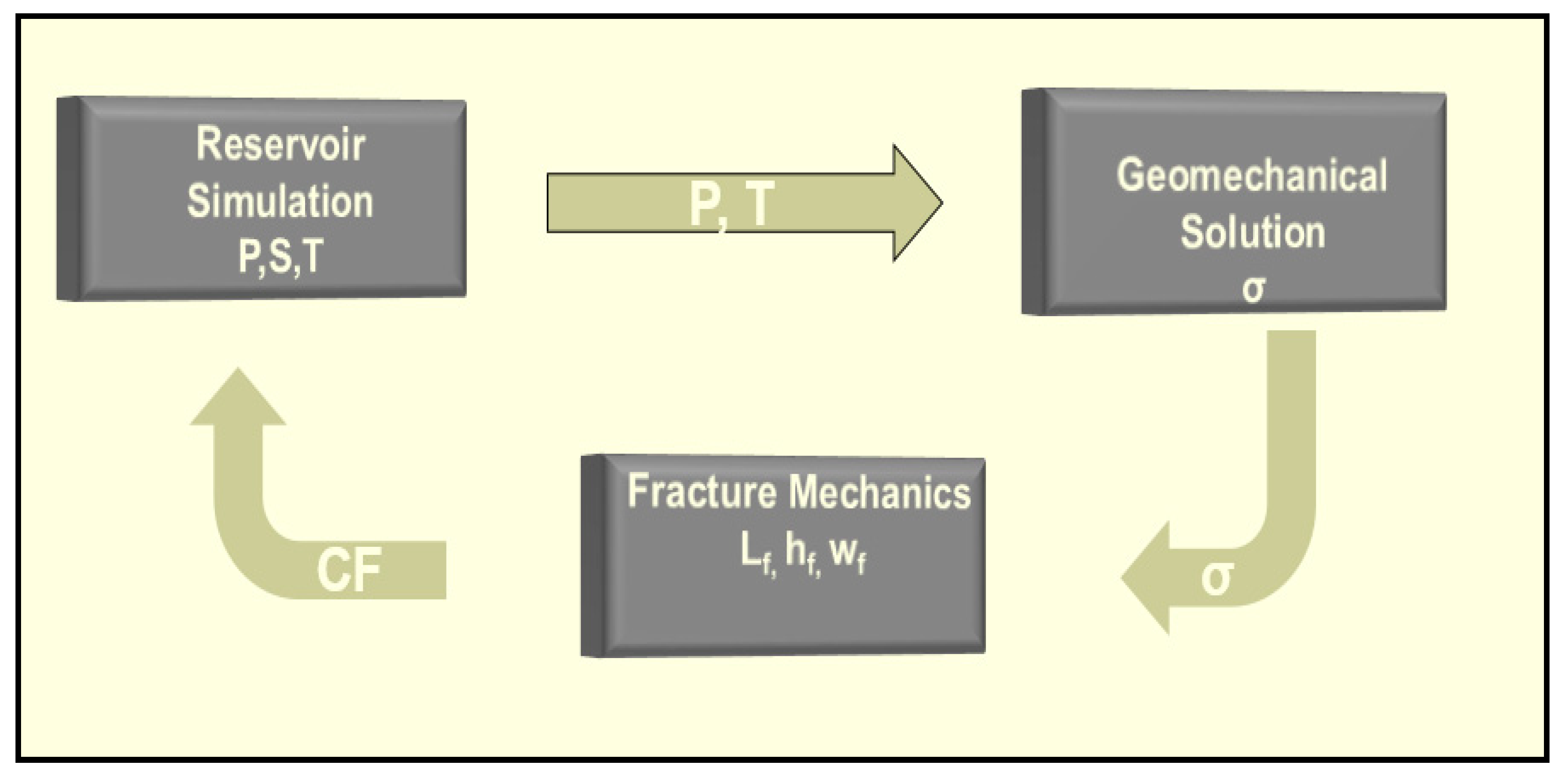
- The modelling equations and assumptions used in the history matching have been detailed to ensure that the essential elements of coupling among the fluid flow, heat flow, geomechanics, and fracture mechanics have been incorporated.
- The received model was converted from an isothermal to a thermal model. The pressure-volume-temperature (PVT) properties were defined at a single temperature. It was necessary to define the fluid PVT properties across the full range of temperatures encountered during the injection of the cold water into the reservoir.
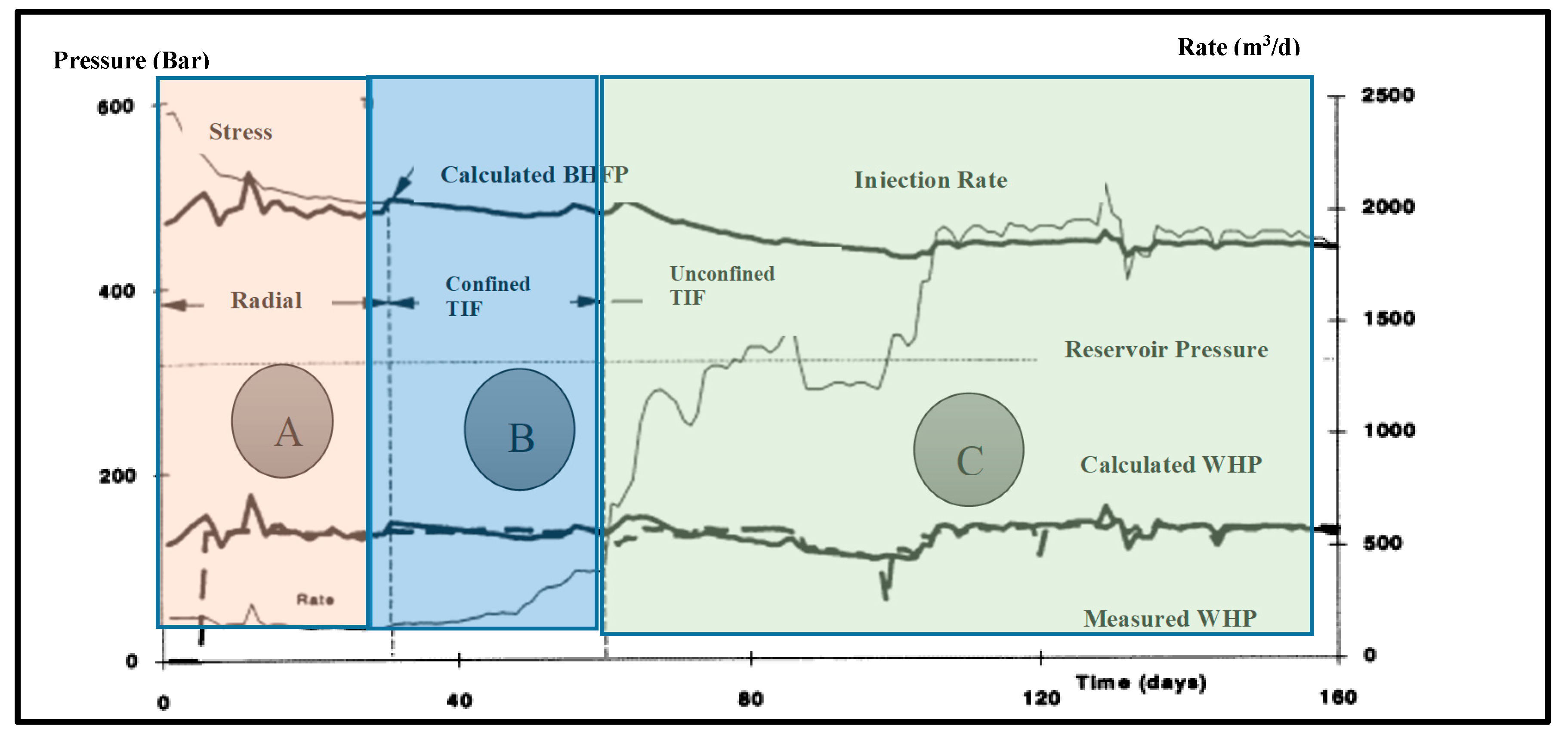
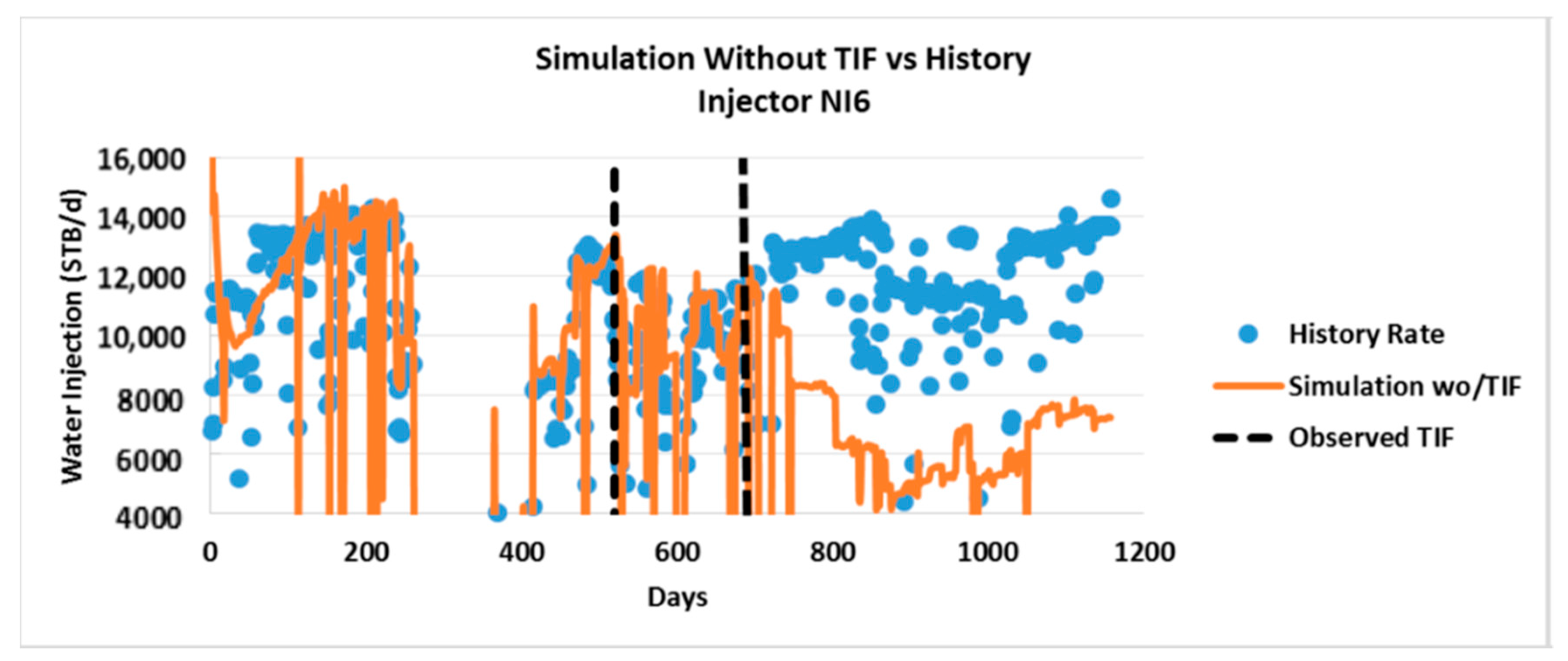
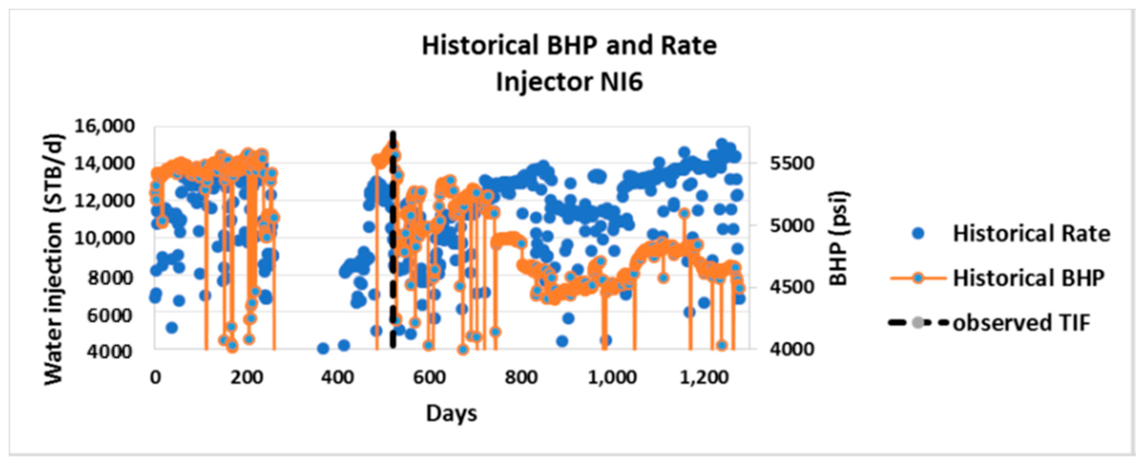
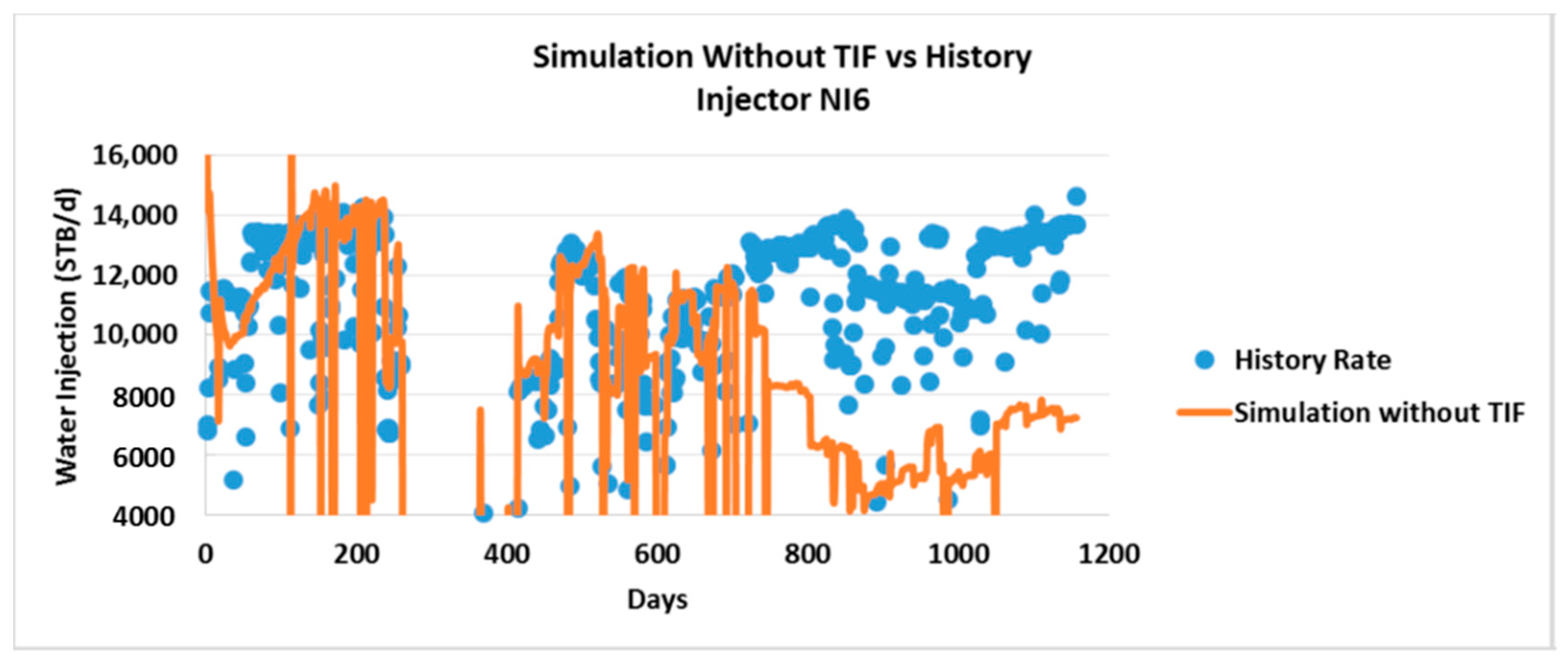
- A simulation was run without TIF modelling and compared to the historical data. This step allowed for an examination of the performance of the injector and identification of any potential indication of a TIF. An increase in the injection rate corresponding to a reduction in BHP can be used as an indicator of a TIF formation, especially if there is a reduction in temperature in the fluid injected. The values calculated for the reservoir pressure around the injectors and bottom hole injection pressure did not match to reliable data at this stage.
- In-situ stresses (in this case, for the N Field) were estimated from the data obtained from offset wells supplied by the operator. This included an estimation of vertical stress, orientation of the minimum horizontal stress, and estimation of the magnitudes of the minimum and maximum horizontal stresses.
- Dynamic mechanical properties of the rock (such as the Young’s modulus, Poisson’s ratio, toughness, and Biot’s coefficient) were determined using either compressional and shear velocities from acoustic log data provided by the operator, or when necessary, by employing published correlations.
- A TIF was then modelled to assess uncertainties and data reliability, as well as to investigate the possibility of TIF initiation and propagation using parameters obtained in steps iv and v. The results were then compared to the historical data.
- The history matching was then finalized after rectifying uncertain parameters (e.g., reservoir pressure and BHP). Workflows at different levels of the history matching were then used.
4. Thermally Induced Fracture Modelling
4.1. Introduction and Underlying Assumptions
- The importance of flow in the reservoir for long-term TIF growth modelling is not appreciated.
- Large time steps are required for TIF modelling.
- TIFs have much higher leak-off rates.
- Thermal aspects are normally neglected in hydraulic fracture models (i.e., the thermo-elastic stress is not considered).
- Flow rate, pressure, and temperature of the injected fluid;
- Mechanical properties of the rock;
- Thermal properties;
- Reservoir properties; and
- In-situ stresses
- The difference between the BHP and minimum horizontal stress;
- Rock mechanical properties (e.g., Poisson’s ratio and Young’s modulus); and
- Critical stress intensity (KIC) (i.e., rock toughness).
- Formation rocks were continuous and linearly elastic;
- Mechanical properties of the rock were homogenous and isotropic;
- TIFs develop as planes (i.e., vertical TIFs were oriented orthogonally to the direction of the minimum horizontal stress);
- Reservoir porosity and permeability were independent of fluid pressure and formation stresses;
- TIF propagation was controlled by linear elastic fracture mechanics (LEFM) (i.e., KIC was a measure of the intensity of the stress near the tip of the TIF required for TIF propagation to occur);
- Stress regime was normal faulting: σv > σHmax > σhmin; and
- Magnitudes of the in-situ stresses varied with the depth.
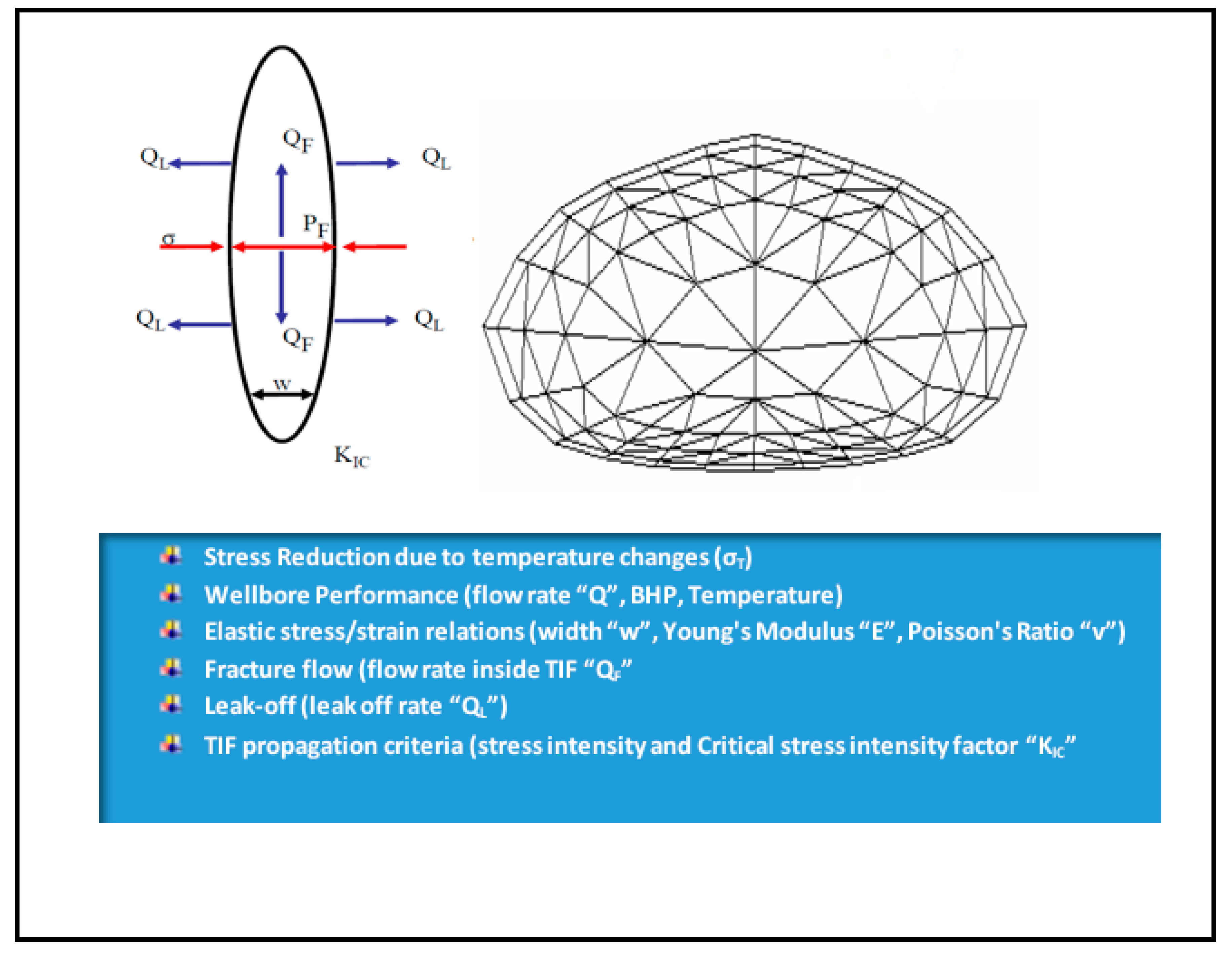
- Elasticity equations that related the pressure on the TIF’s tip to its width;
- Fluid flow equations that related the fluid flow and pressure in the TIF;
- Geomechanical equations that calculated the in-situ stresses, accounting for the effects of temperature and pressure changes on the reservoir stress field; and
- A TIF propagation criterion that related the stress intensity at the TIF tip to the critical stress intensity factor for the rock (KIC).
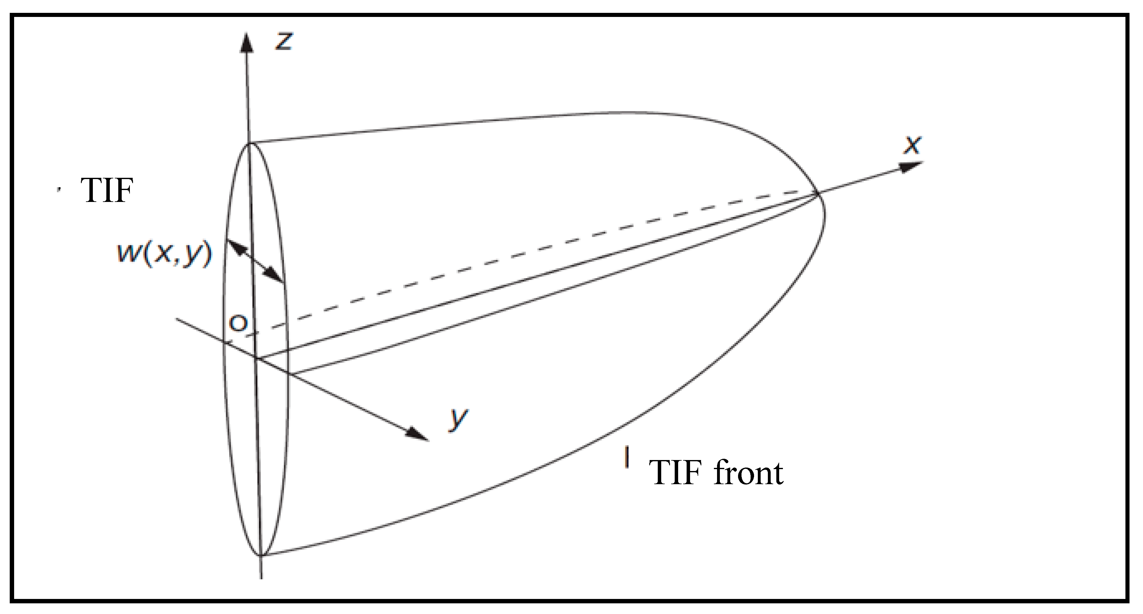
4.2. Elasticity Equation
| Total minimum horizontal stress normal to the TIF plane (y-direction in Figure 10) (psi) | |
| Fluid pressure along the TIF | |
| TIF width (ft) | |
| Shear modulus (psi) defined by the Young’s modulus (E) and Poisson’s ratio (). G is defined as: |
| Poisson’s ratio | |
| Young’s modulus (psi) | |
| Distance between the source point (x’, z’) at which the integrand is evaluated and the field point at which the pressure is evaluated (x, z) (see Figure 10). R is defined as: |
4.3. Fluid Flow Equation
| Pore pressure at far field (psi) | |
| Time increment (sec) | |
| M | Mobility connection factor, defined as: |
| Reservoir permeability in the y-direction (see Figure 10) | |
| Water relative permeability (md) | |
| Water viscosity (cp) |
4.4. Geomechanical Equations
4.5. Stress Calculation in the 3D FD Main Reservoir Grid
| Initial minimum horizontal stress (psi) | |
| Thermo-elastic stress due to temperature change (psi) | |
| Poro-elastic stress due to pressure change (psi) | |
| Total stress reduction due to temperature and pressure change (i.e., sum of the thermo-elastic and poro-elastic stresses) (psi) |
| Pressure difference between the flooded zone and reservoir pore pressure | |
| Temperature difference between the injected fluid and reservoir (°F) | |
| Poro-elastic constant (psi/psi), defined by: |
| Grain Compressibility (psi−1) | |
| Bulk Compressibility (psi−1) | |
| Thermo- elastic constant (psi/°F) defined by: |
| Thermal expansion coefficient (1/°F) | |
| Goodier displacement potential |
4.6. Stress Calculation for the 2D TIF Surface
| Reservoir temperature (°F) | |
| TIF surface temperature (°F) |
4.7. TIF Propagation Criterion
| Critical width at a fixed distance () from the tip of the TIF (ft) | |
| Defined at a small distance from the tip of the TIF (ft1/2) (see Figure 4) | |
| Critical stress intensity factor ((rock fracture toughness)) (psi ft1/2) |
4.8. Solution Method
- The combined FE equations solver was supplied by a total rate (Qf).
- The geometry of the TIF was iterated until a constant TIF geometry was found (i.e., = ). The pressure at the center of the TIF (PF) was returned and another level of iteration performed.
- The iteration continued until (PF) and (Qf) were consistent with the total well injection rate and BHP.
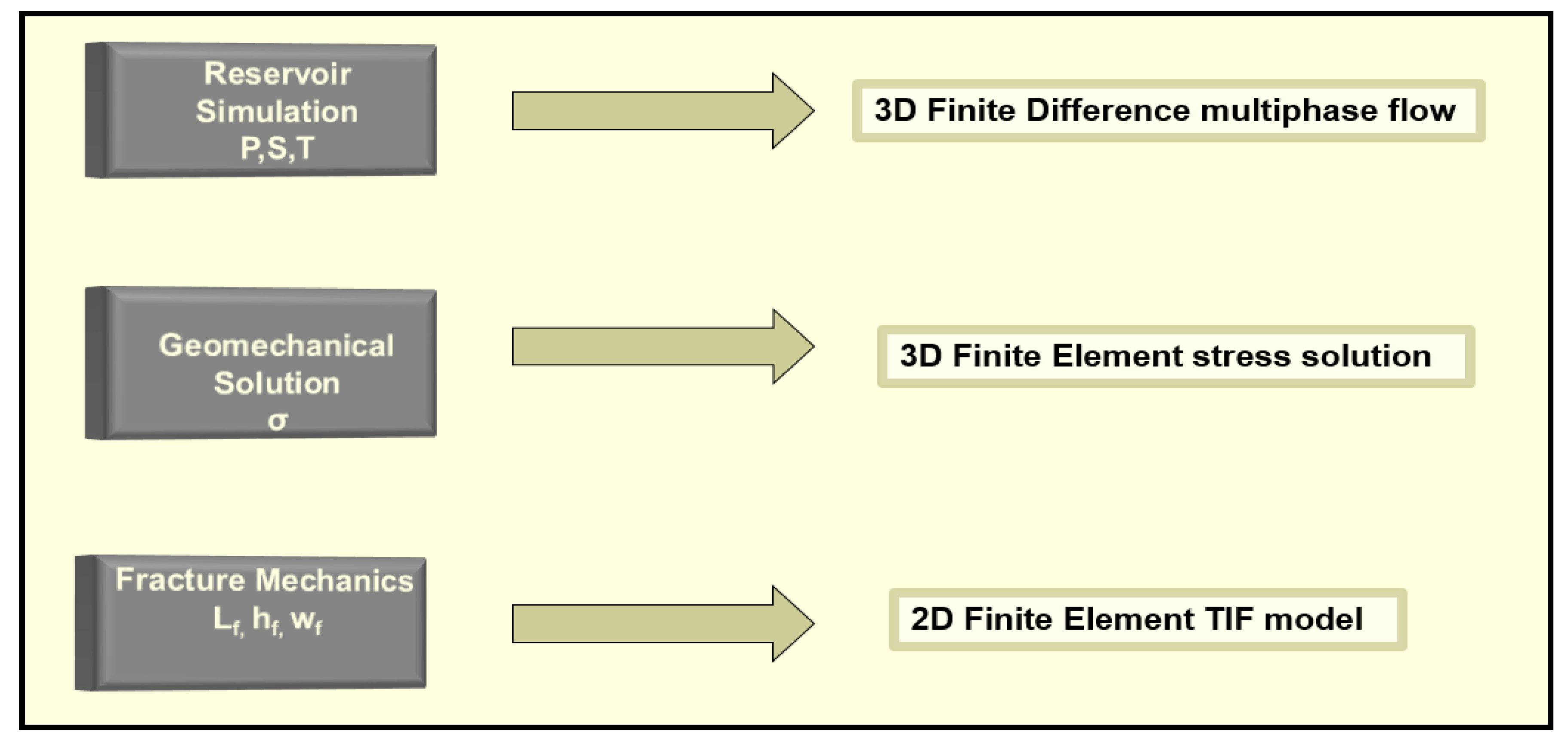
4.9. Implementation Workflow
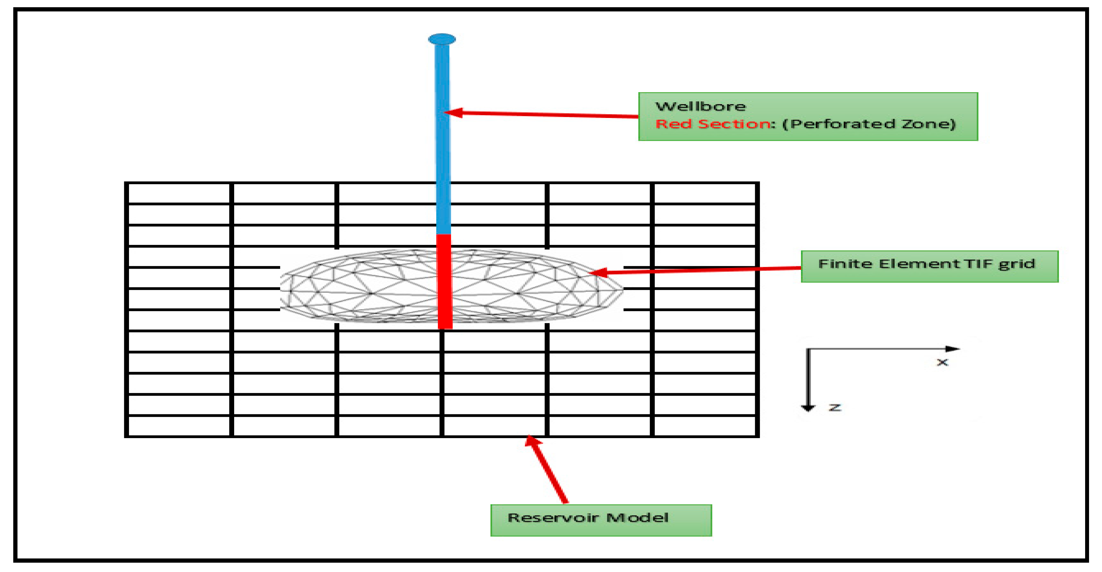
- Reservoir model: A multiphase 3D fluid flow (pressure and saturation) model created via an FD method and using black-oil pressure, volume, and temperature variables.
- Geomechanical solution: An FD method was employed to solve 3D stresses in the rock within the reservoir. The solution used the Goodier displacement potential method, which assumes zero displacement around the reservoir model (i.e., at the reservoir boundary). Once the stress was calculated for the 3D reservoir model, it was then interpolated into the 2D TIF model.
- TIF model: this was an FE grid with triangular internal and quadrilateral boundary elements (see Figure 11). The FE fluid flow and elasticity equations within the TIF were solved iteratively to obtain the TIF widths. The TIF propagation criterion was then applied to define the TIF shape and dimensions.
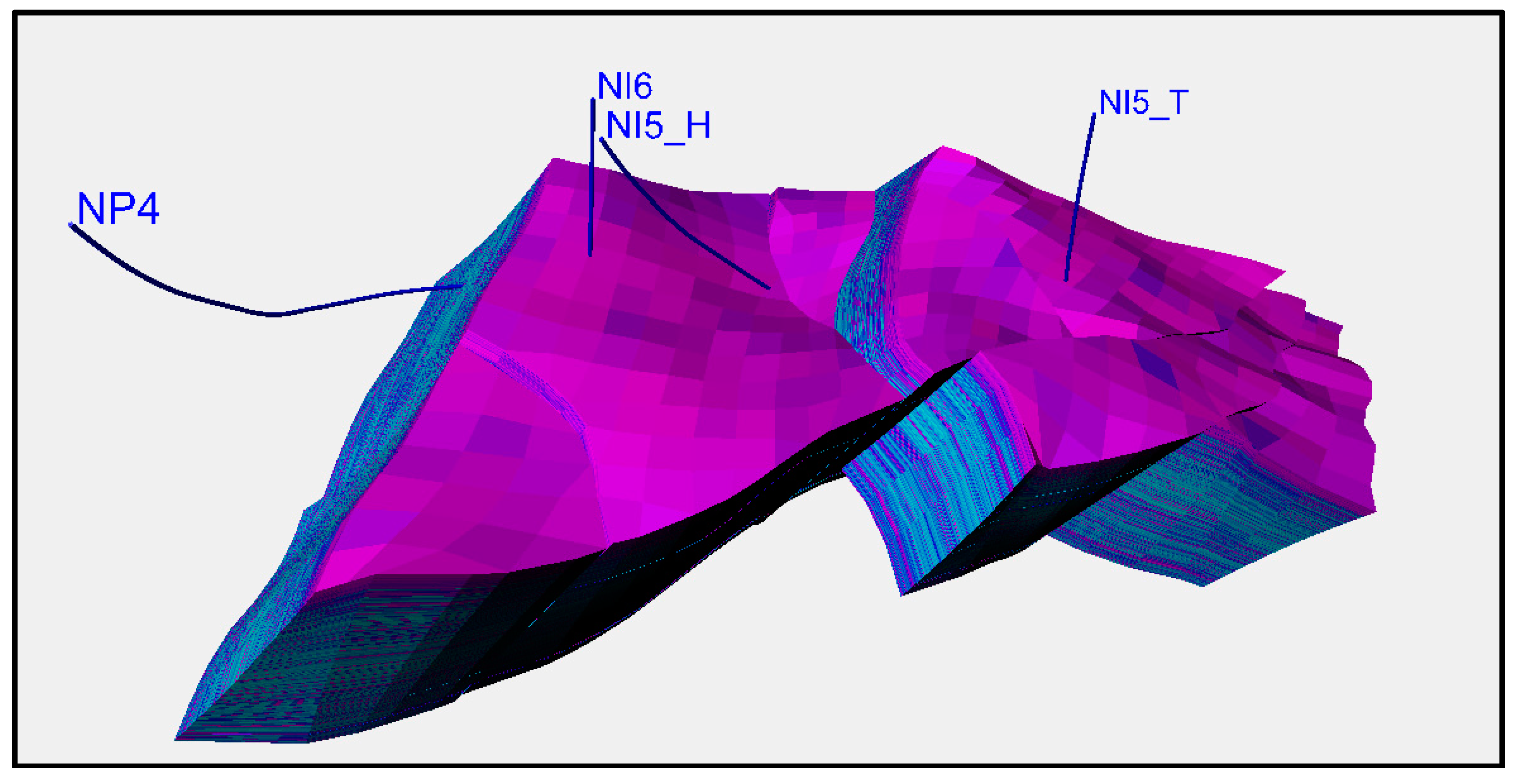
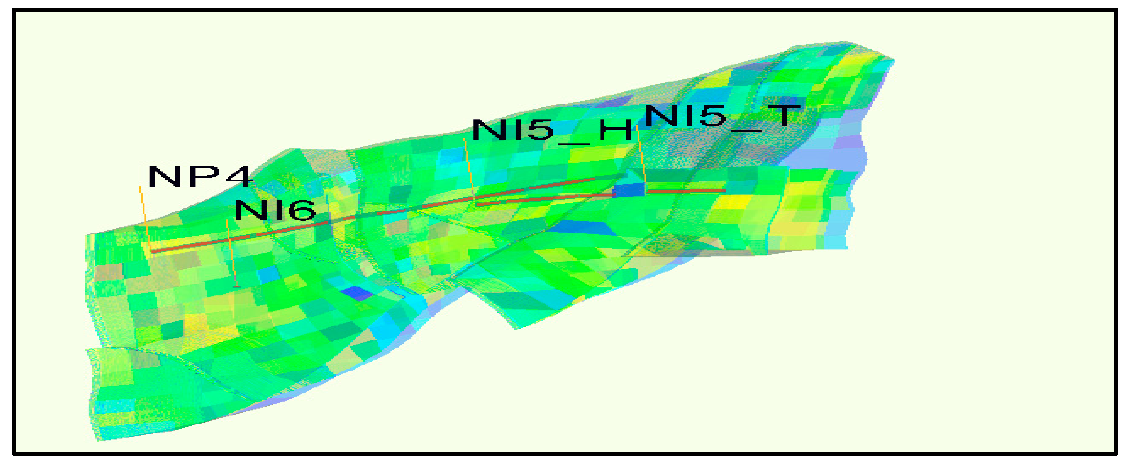
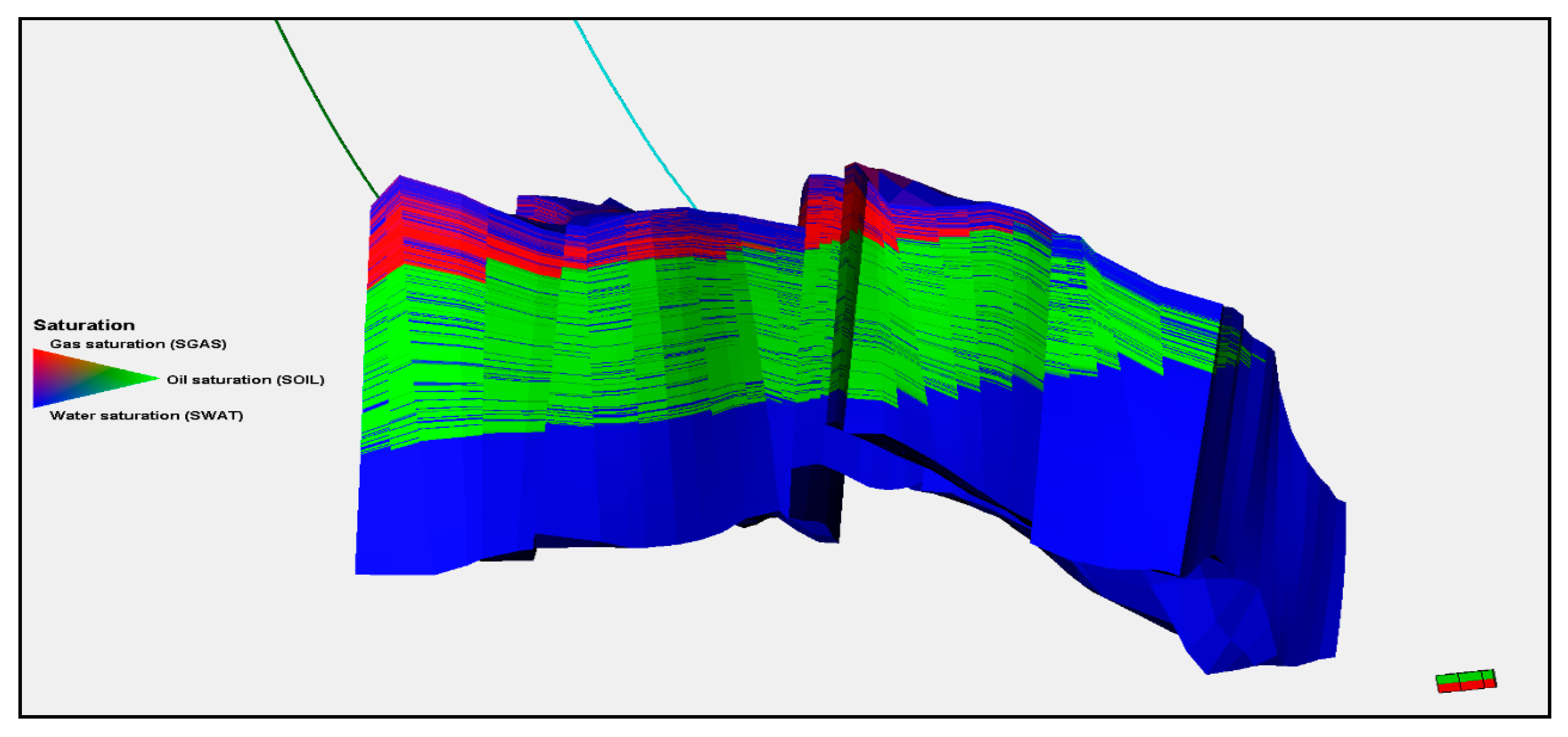
5. Sector Model Description
N Field Sector Model Description
6. Converting the Isothermal Reservoir Model to a Thermal Model
7. History Matching the N Field Sector Model Without a TIF
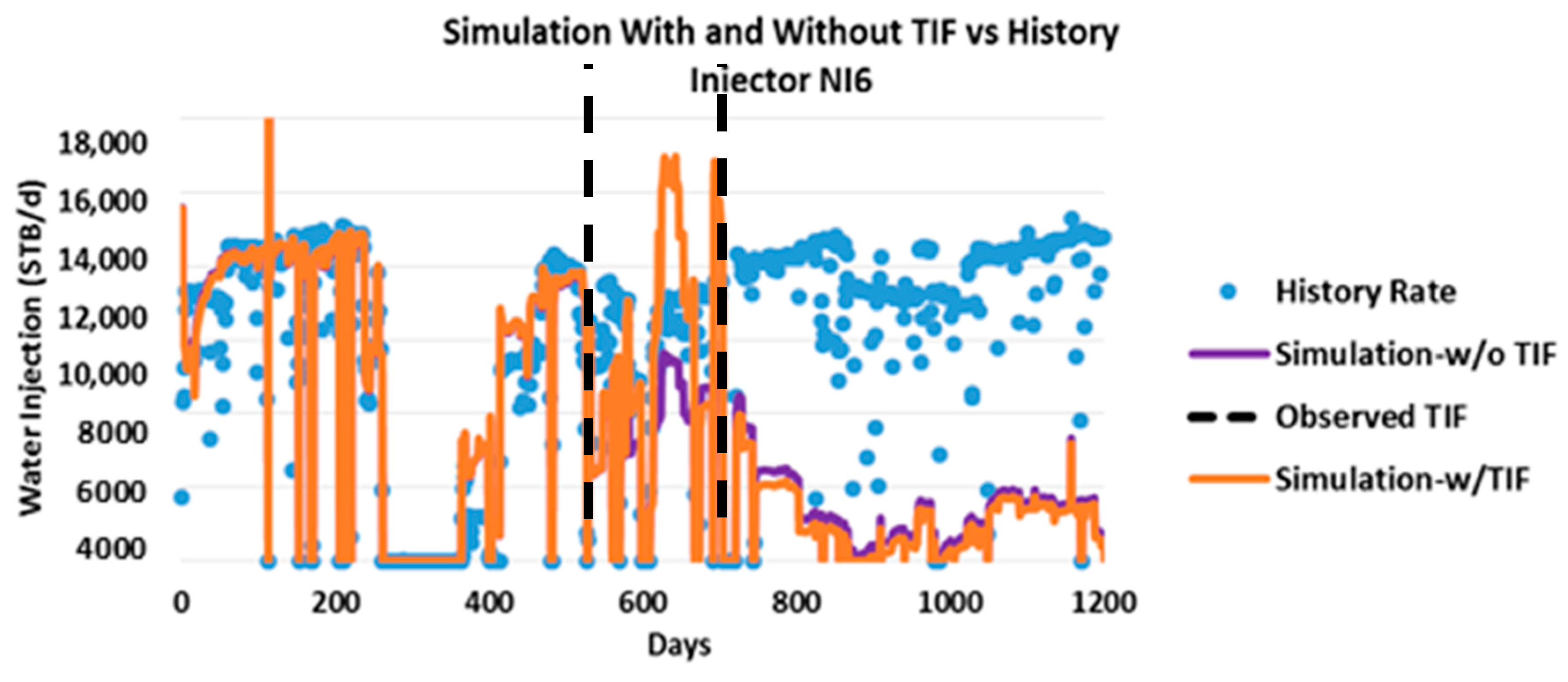
- How did Injector NI6 perform during the entire period?
- When did the deviation from the historical data occur?
- Did the deviation correspond to the TIF occurrence period observed?
8. In-Situ Stress
- The direction of the principle in-situ stress in the “N” field is vertical
- The stress regime was normal faulting: σv > σHmax > σhmin.
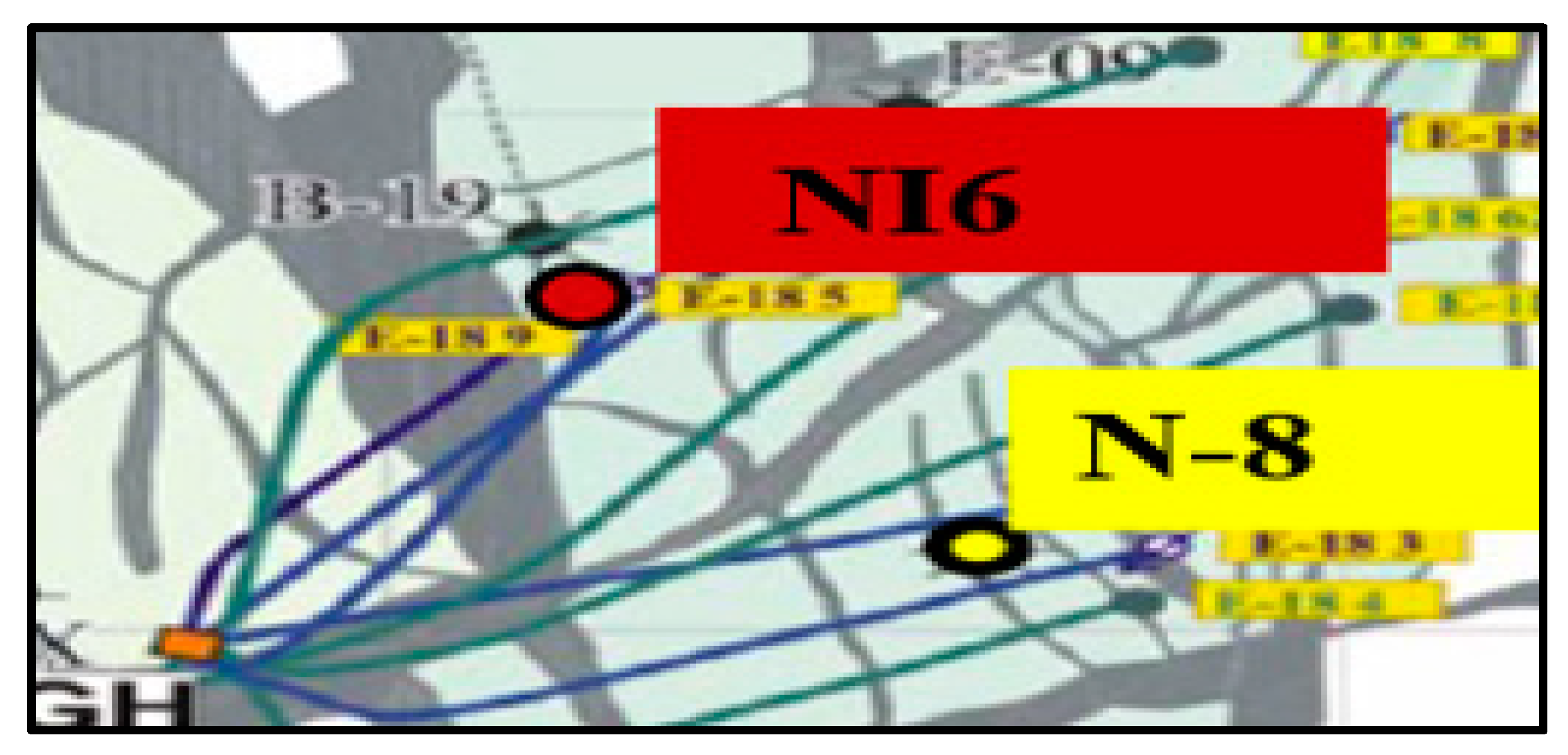
- All measurements and estimations of in-situ stress and rock mechanical properties for Well N-8 were assumed to also apply to Injector NI6.
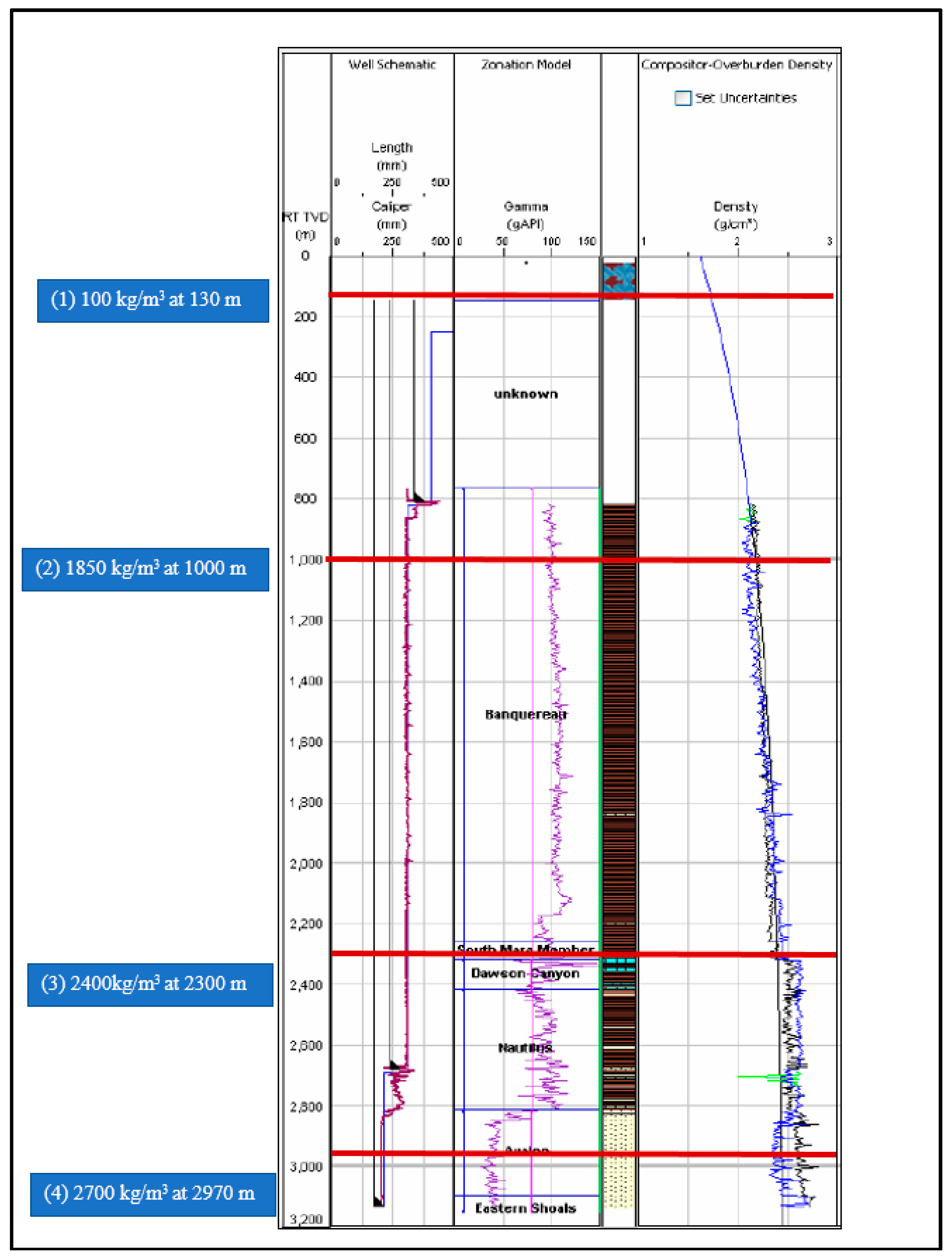
8.1. Estimation of Vertical Stress
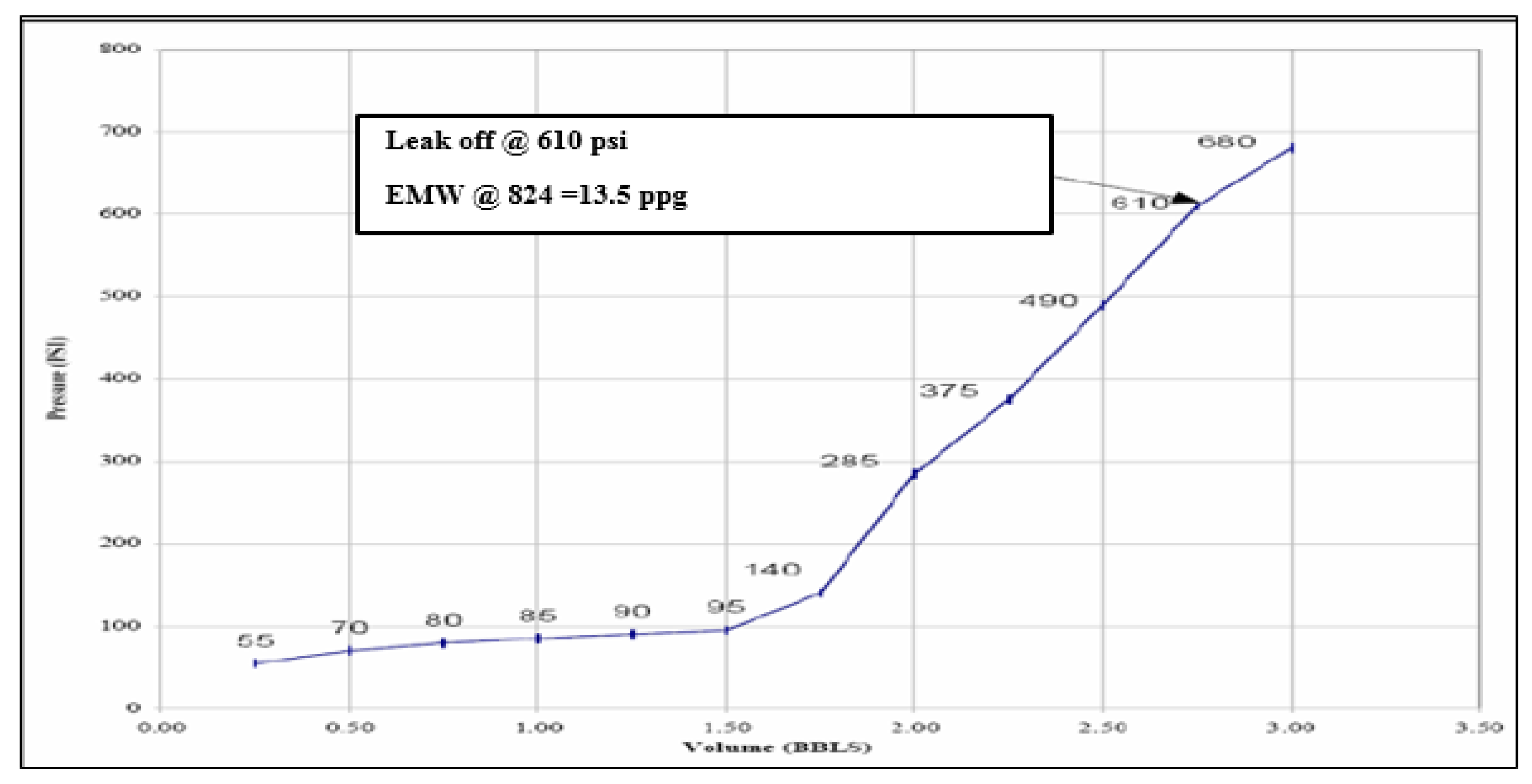
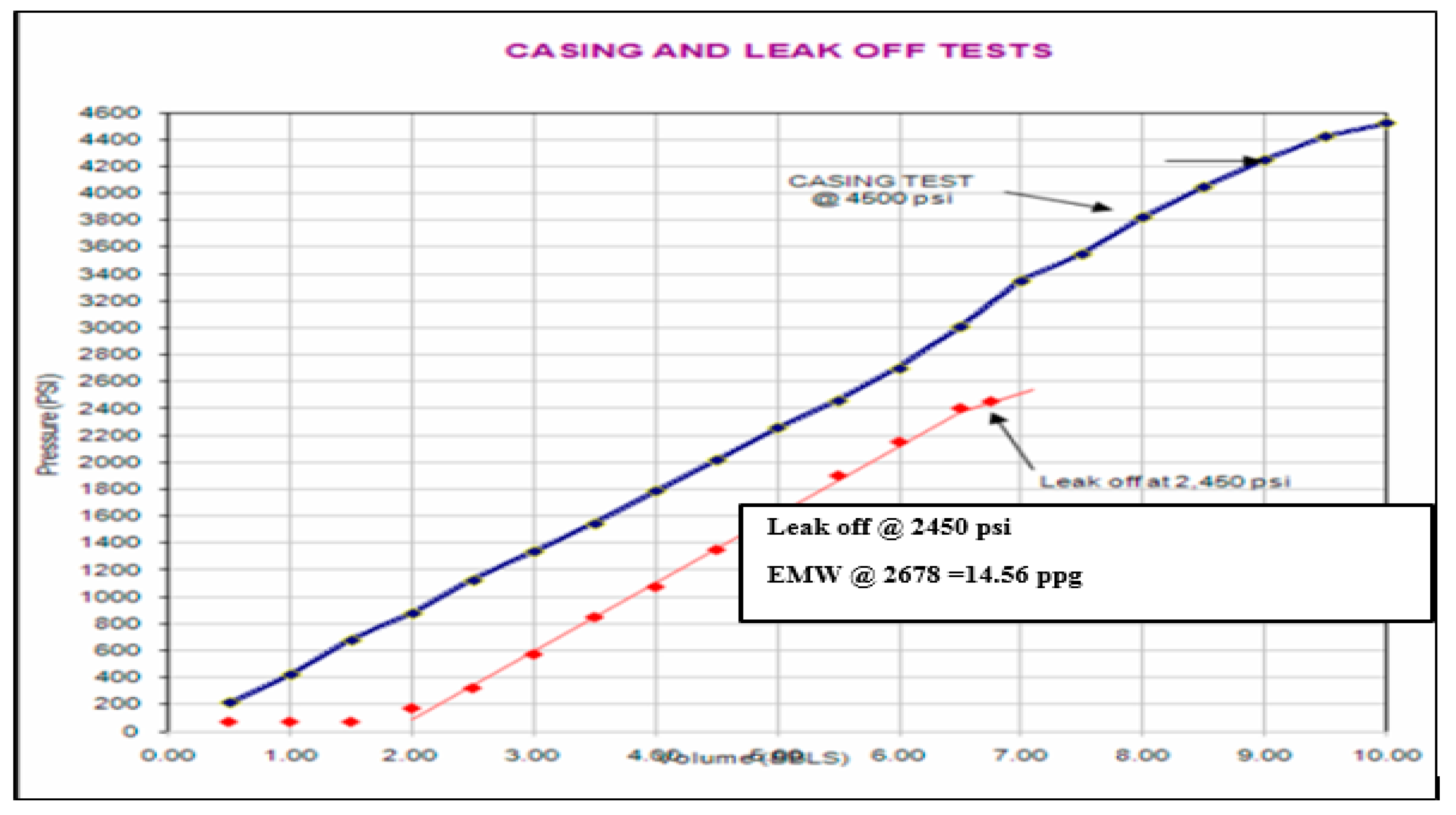
8.2. Magnitude of the Minimum Horizontal Stress
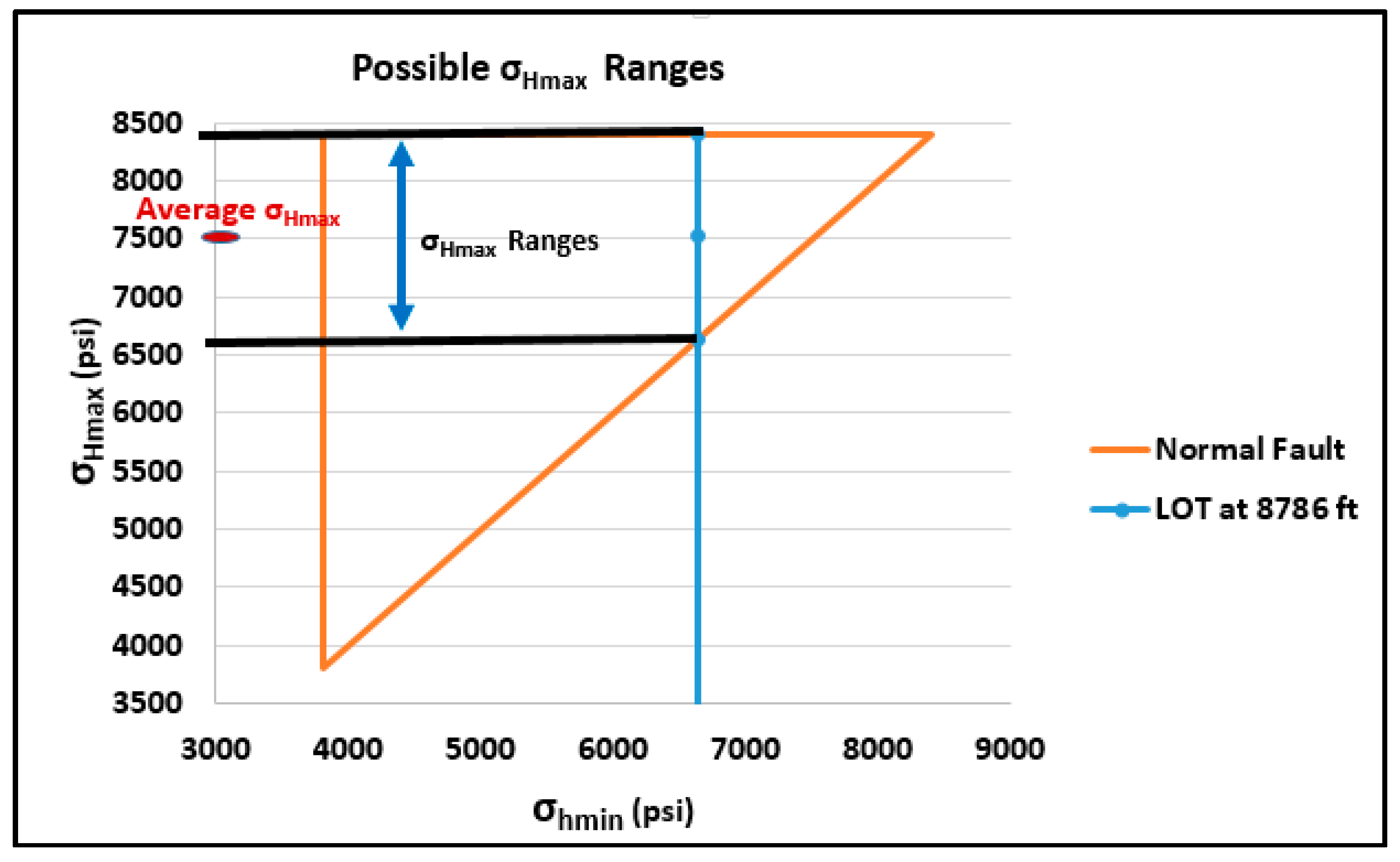
8.3. Magnitude of the Maximum Horizontal Stress
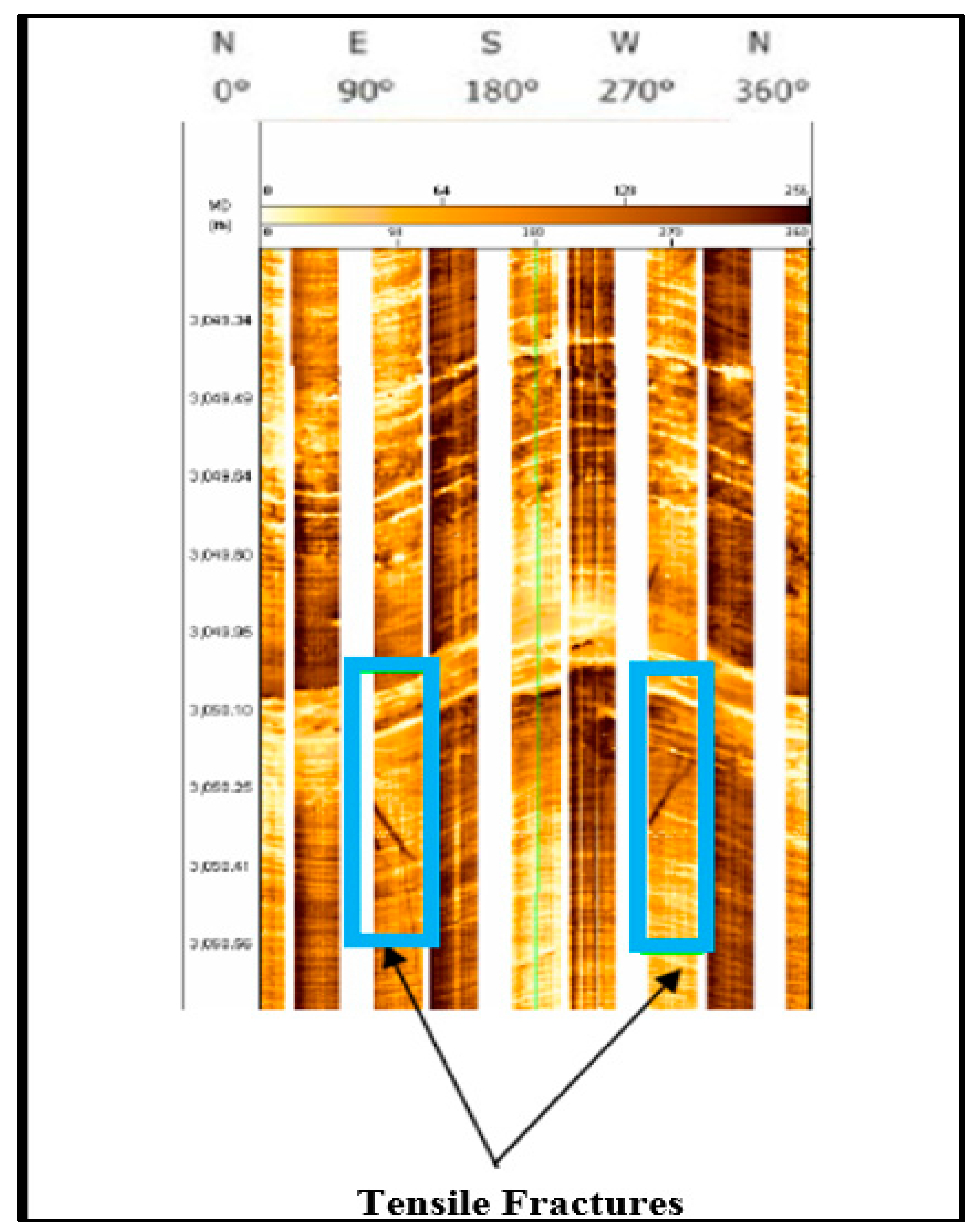
8.4. Orientation of the Minimum Horizontal Stress
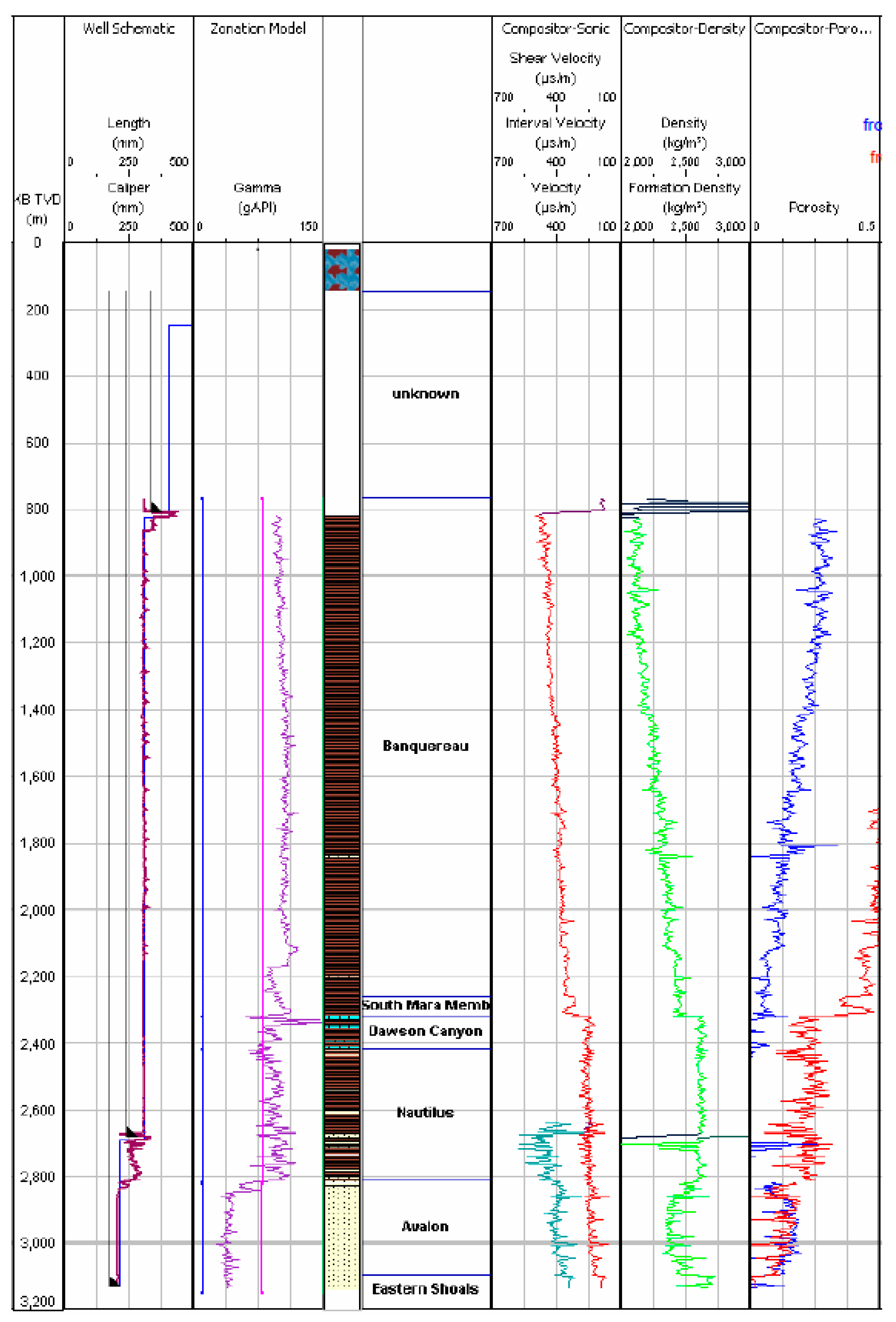
9. Rock Mechanical Properties
9.1. Young’s Modulus and Poisson’s Ratio
9.2. Fracture Toughness
9.3. Biot’s Coefficient
- Biot’s coefficient
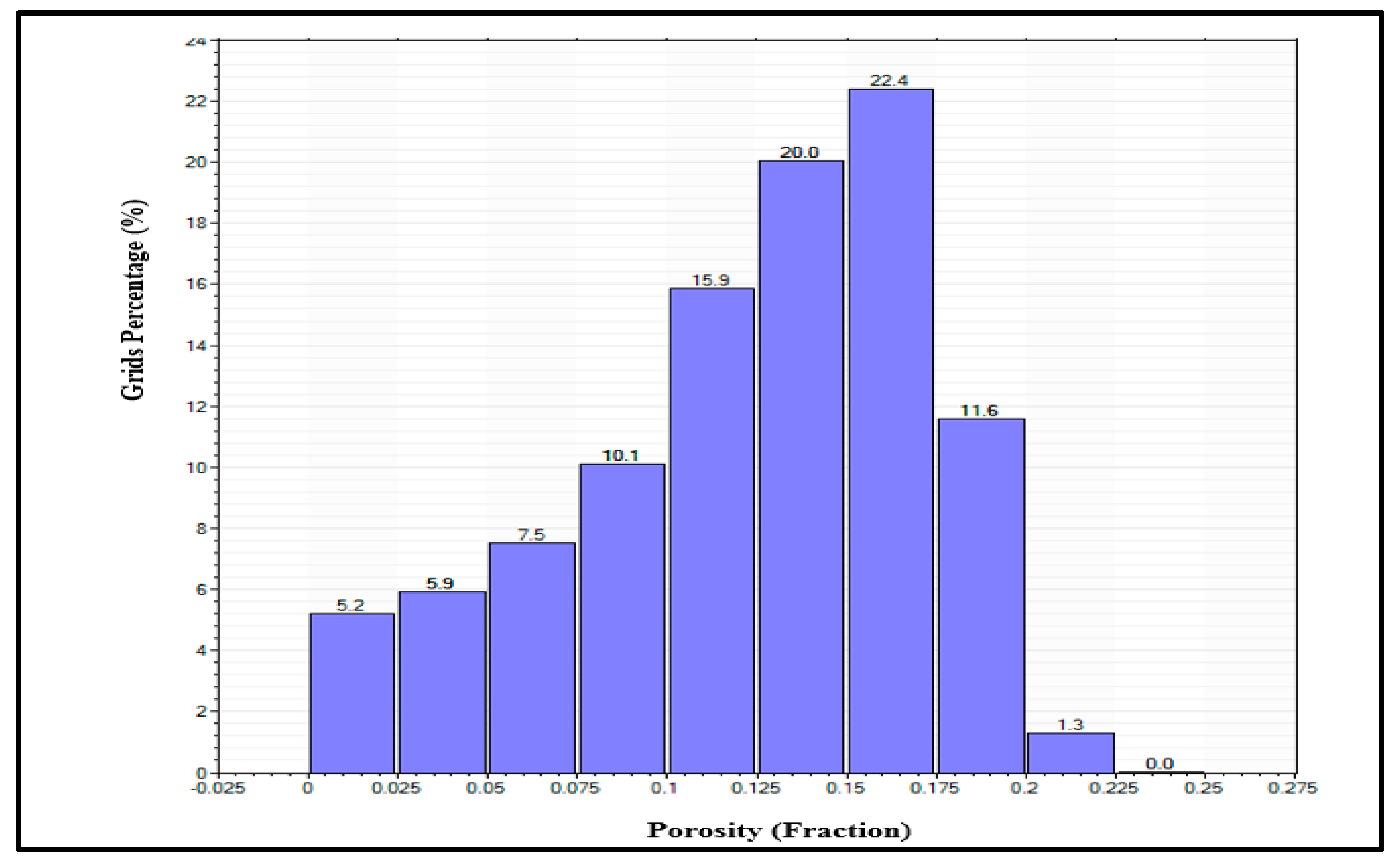
- Porosity
10. Uncertainty Analysis
10.1. Reservoir Pressure
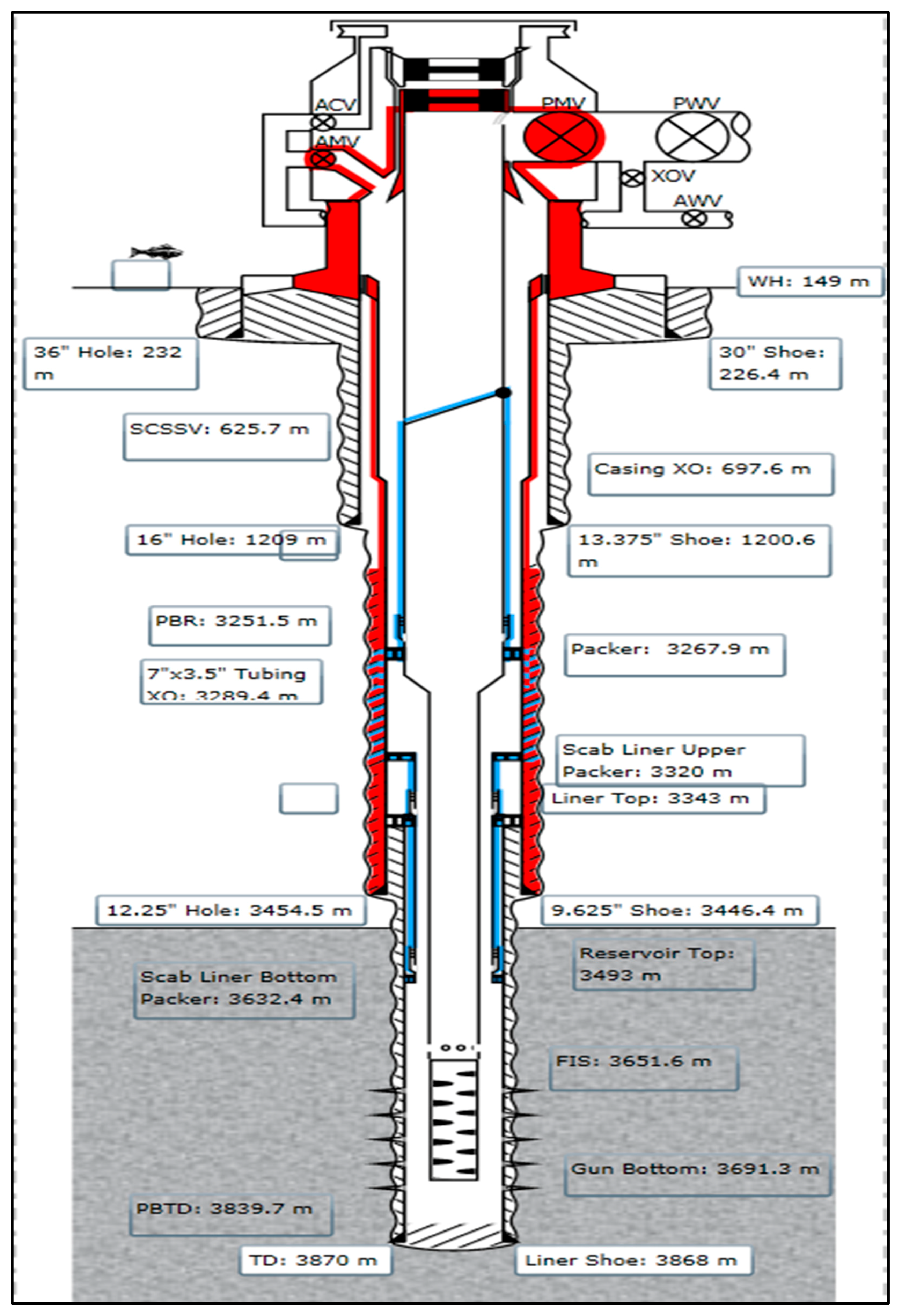
10.2. Wellbore Modelling
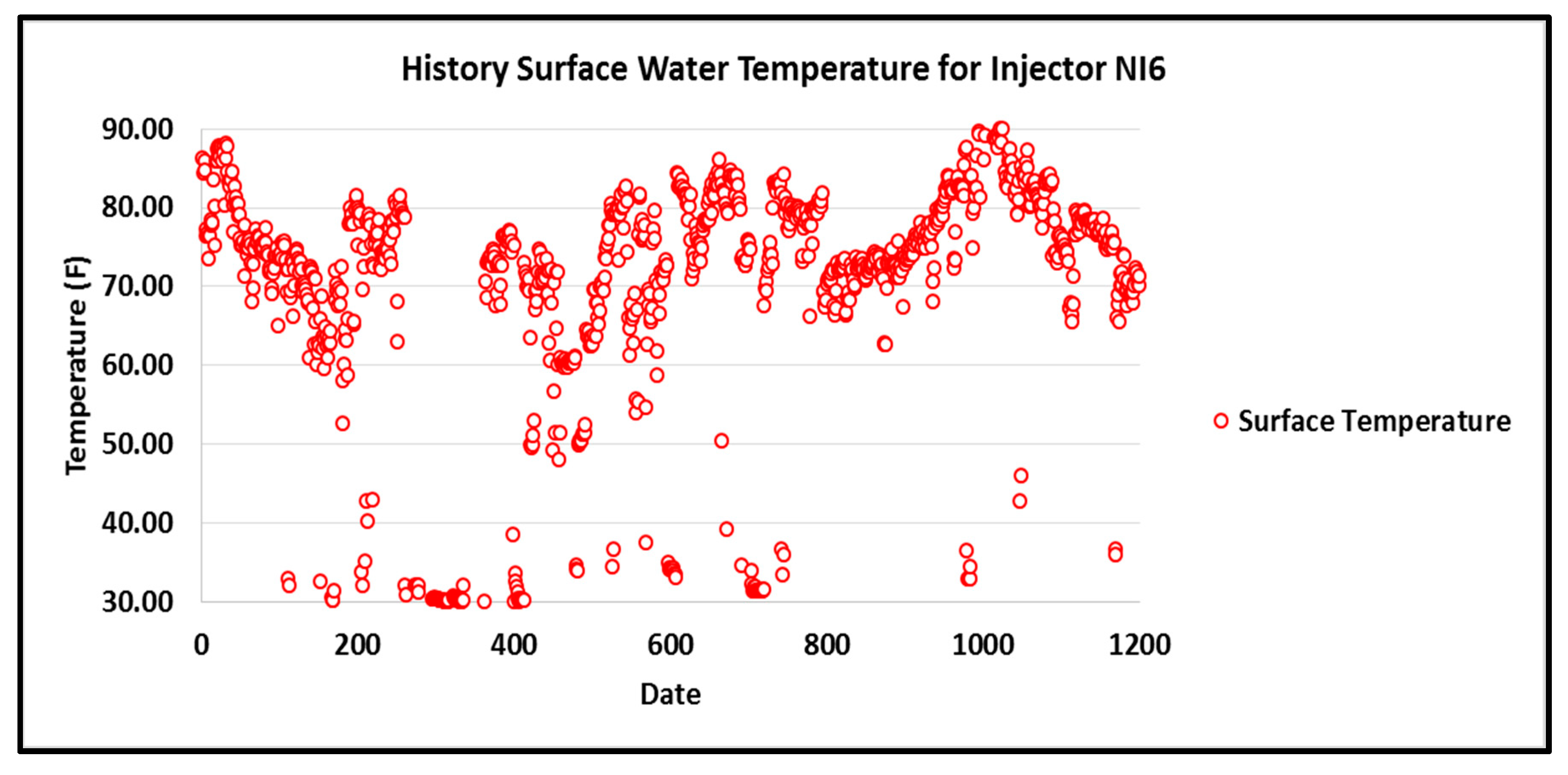
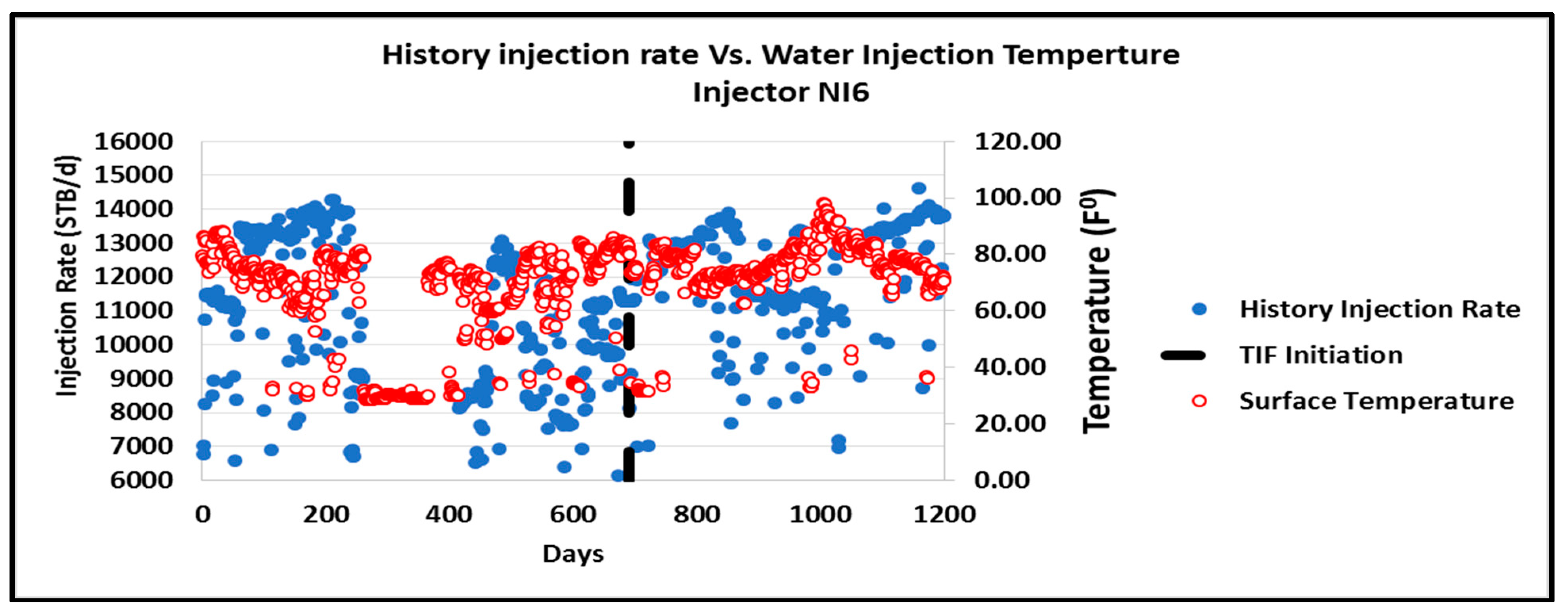
10.3. Type and Surface Temperature of the Injected Water
11. History Matching with the TIF Modelling Workflow
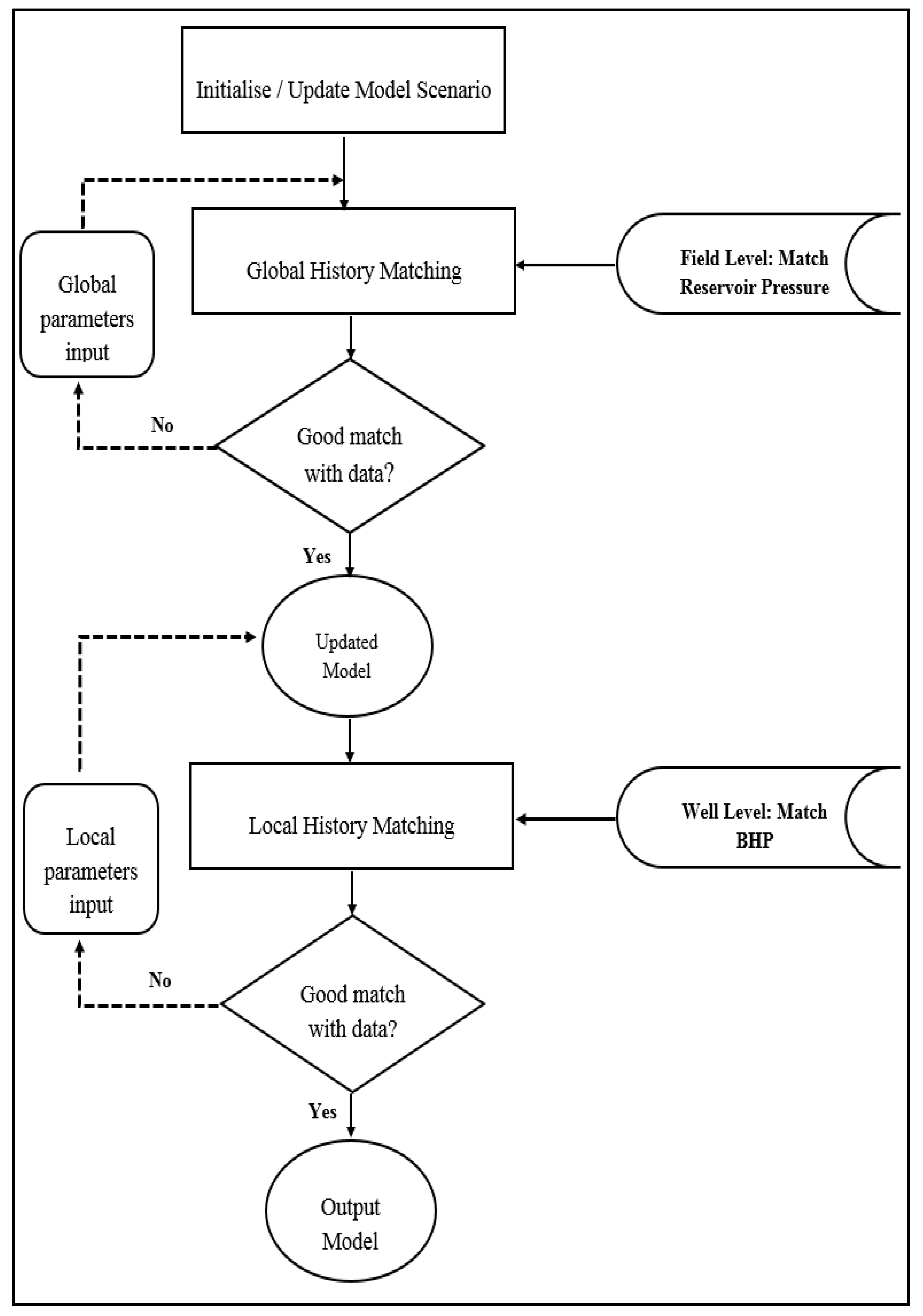
- Figure 32 indicating the workflow used to achieve a good match of the no-TIF simulation and historical data. The injection rate of Well NI6 was not matched at this stage. This workflow is discussed further in Section 11.1 and Section 11.2.
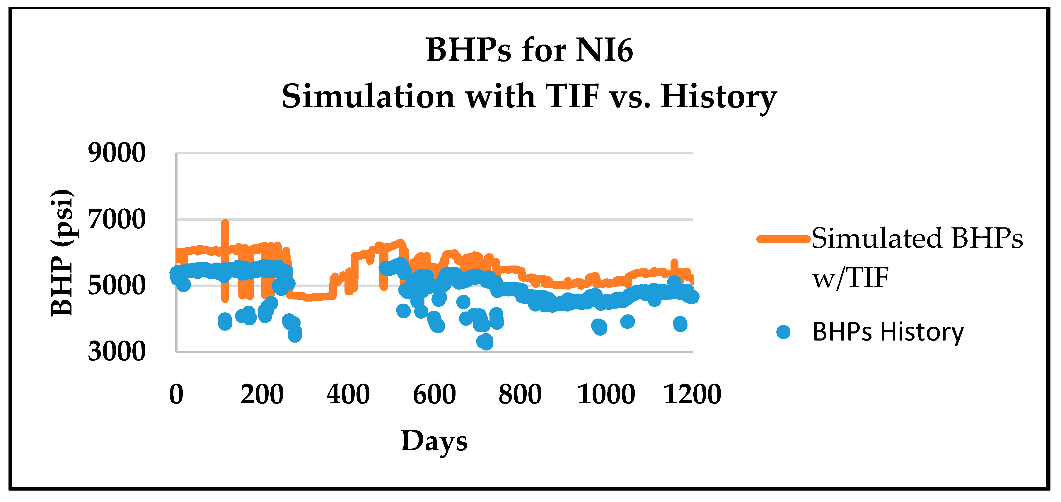
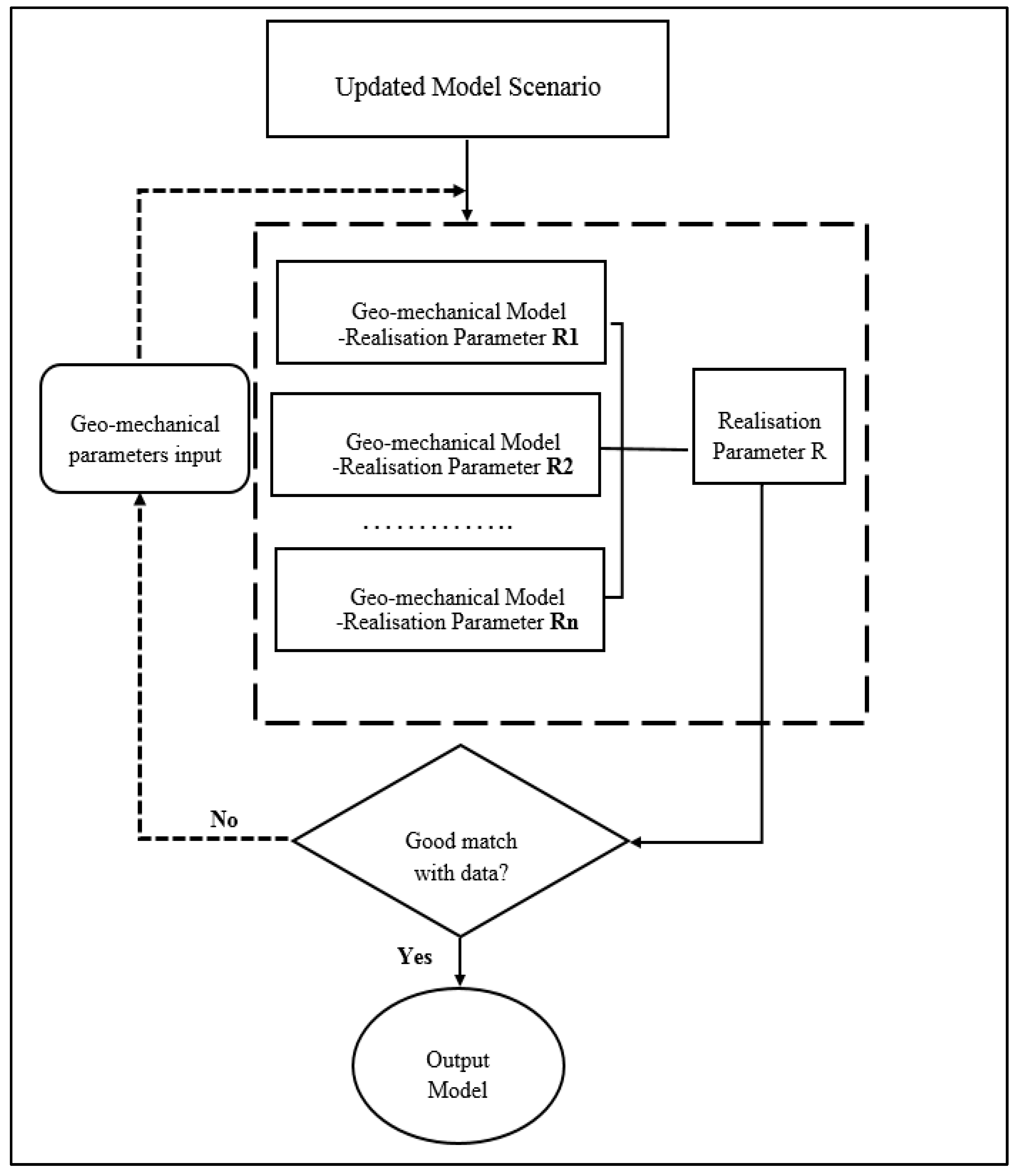
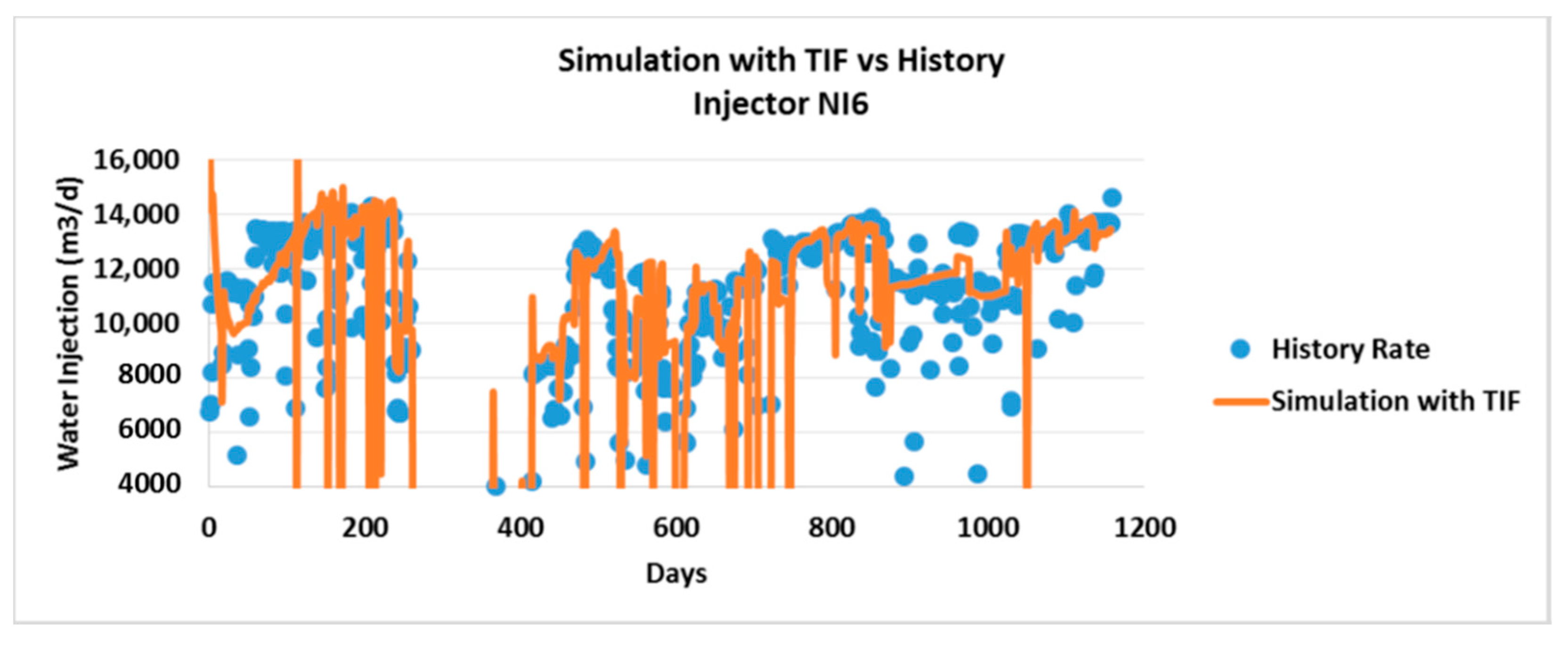
- Figure 33 shows the workflow used to obtain a good history match after a TIF has occurred. The in-situ stresses and rock mechanical properties were matched here. A good match to the injection rate of NI6 was the ultimate goal at this stage. This workflow is discussed further in Section 12.
11.1. Global History Matching
Regional Reservoir Pressure
11.2. Local History Matching
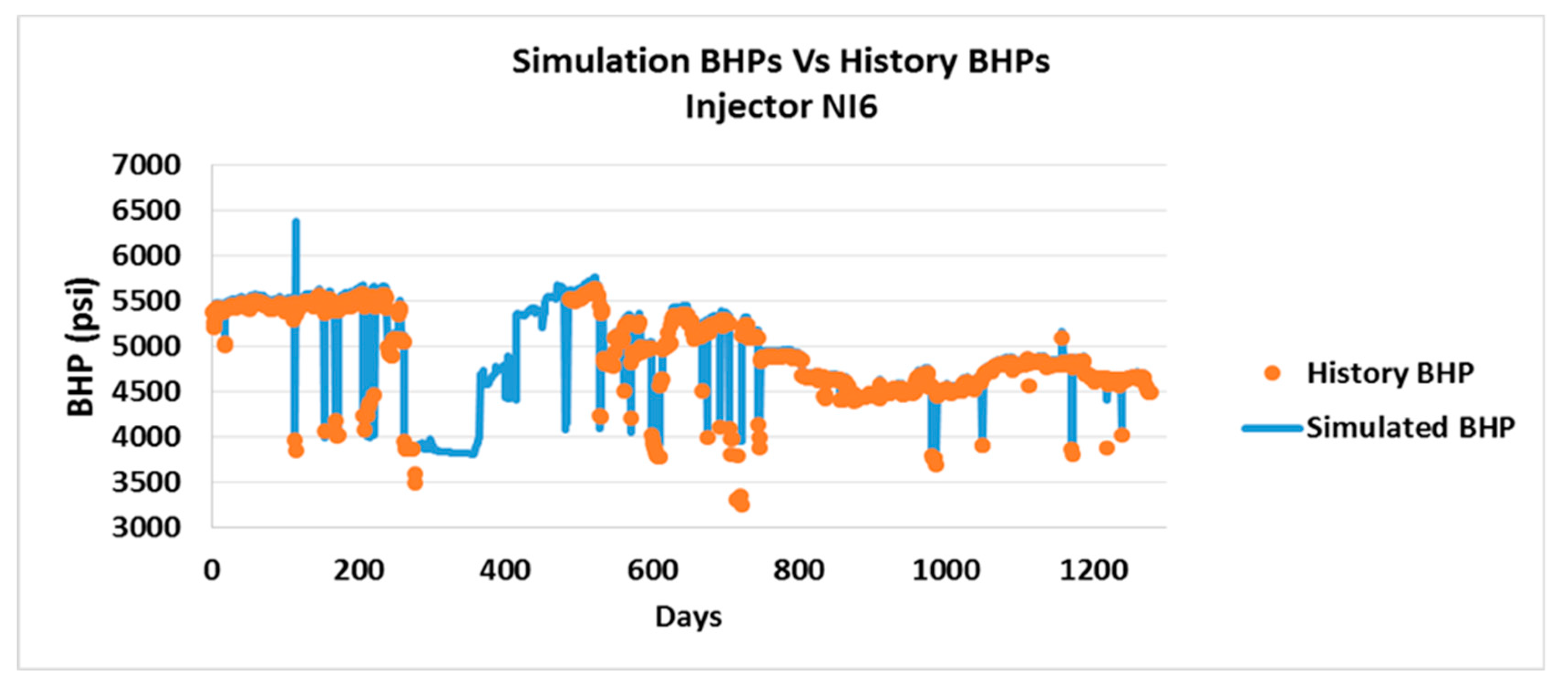
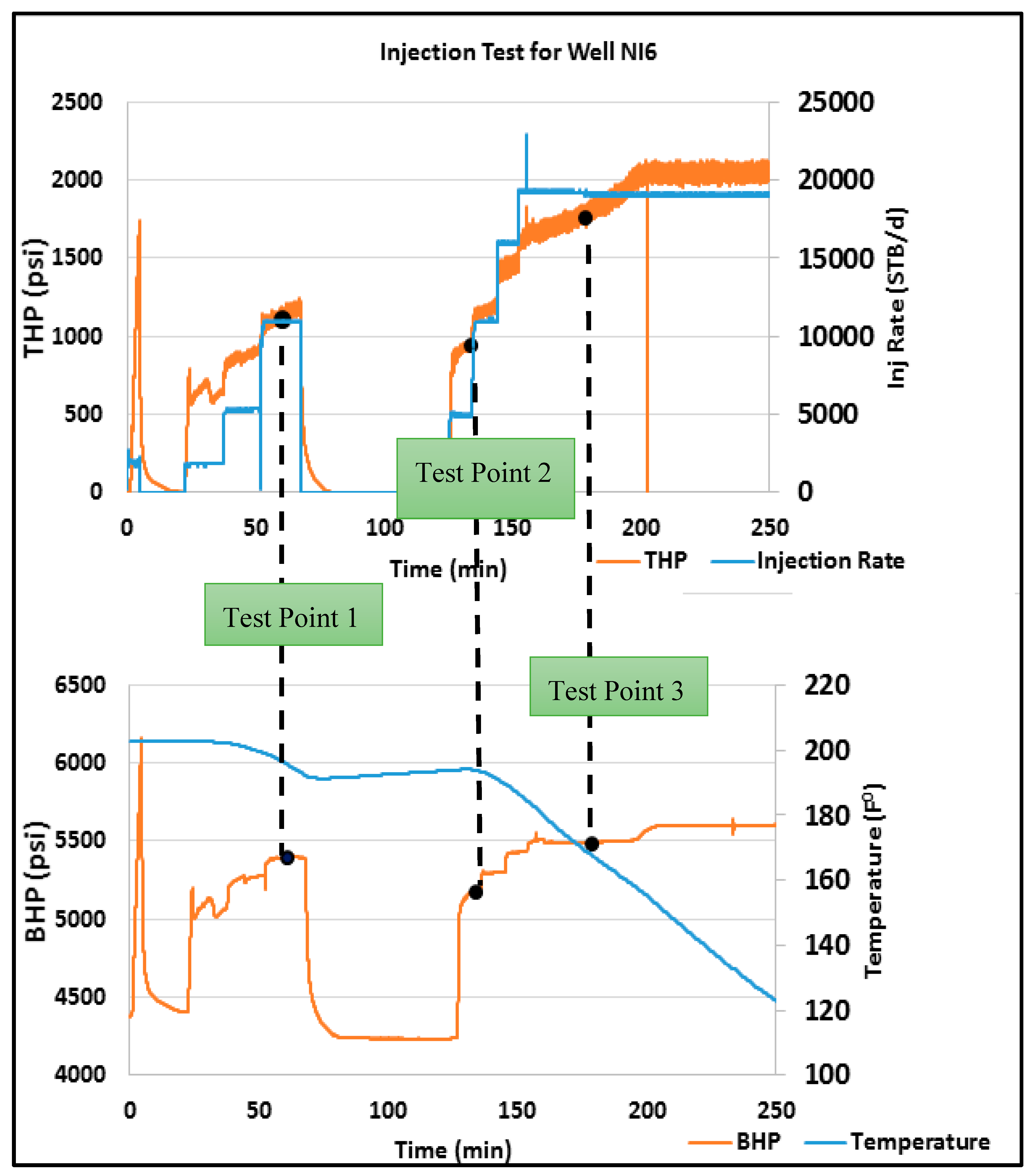
Well NI6 BHP
- A critical review of the raw well test data (see Figure 36) addressed how reliable the measurements were and how the test data compared to the historical trends.
- Three test points from the injection test (see Figure 36) were selected for further analysis
- All vertical lift performance (VLP) correlations in PROPSER were compared and the Petroleum Experts 2 correlation was selected since it reproduced each well test with reasonable accuracy (see Table 2).
- Finally, the simulated BHP successfully reproduced the historical BHP (see Figure 37).
12. Final Matching with TIF Modelling
12.1. Injected Water Temperature
12.2. Geomechanical and Thermal Properties
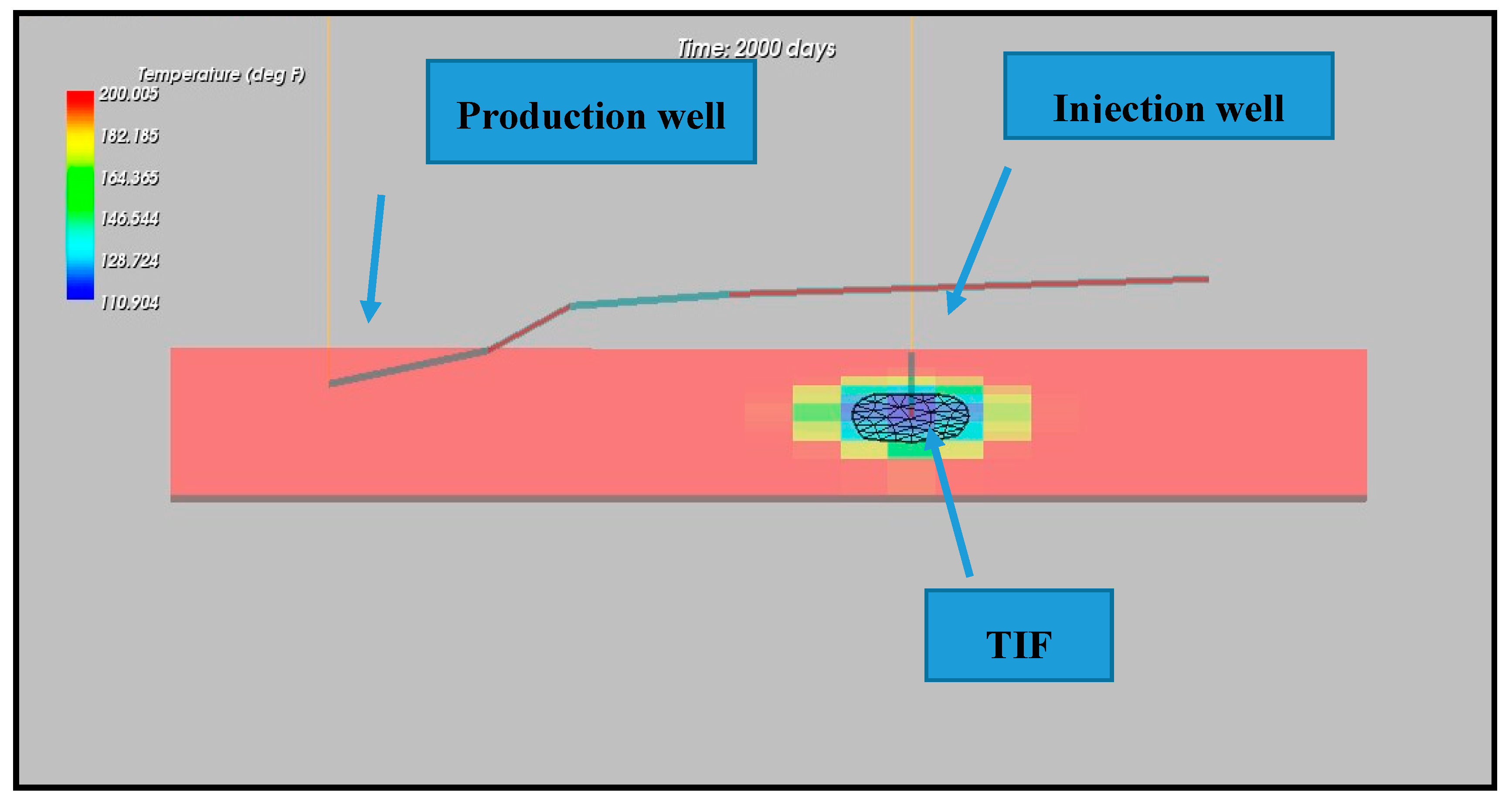
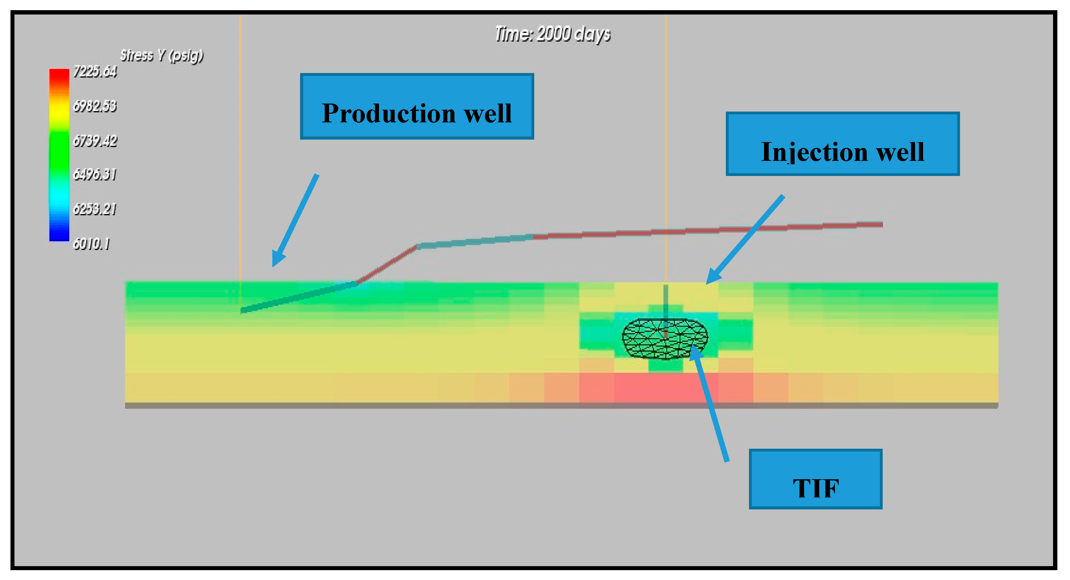
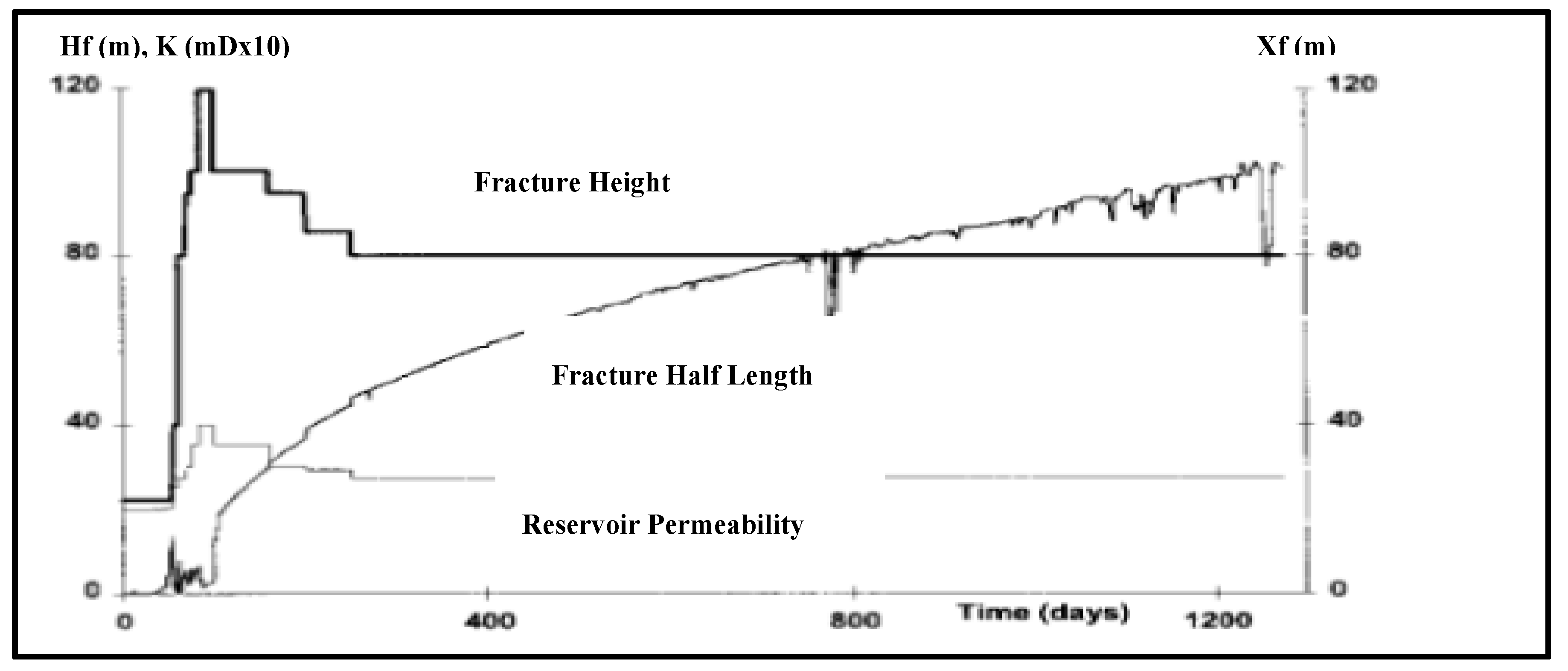
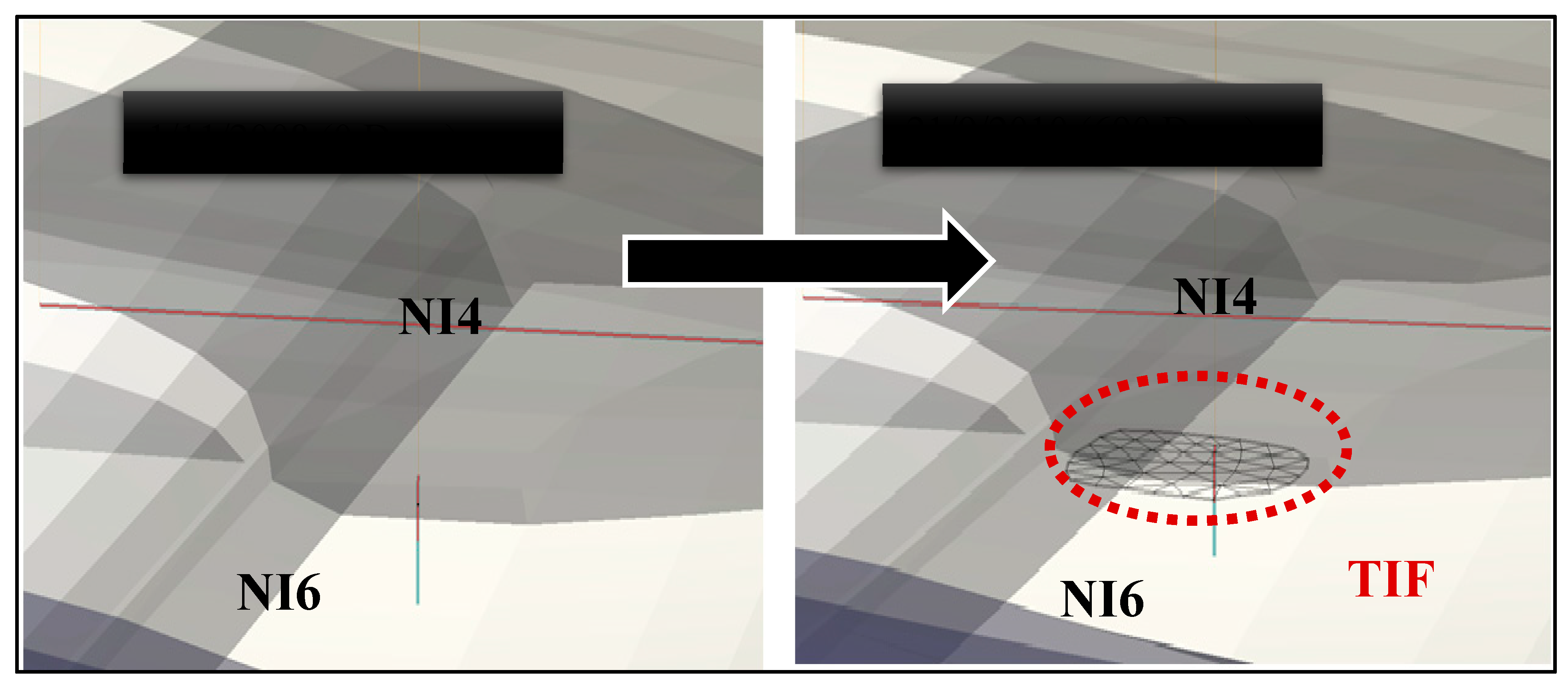
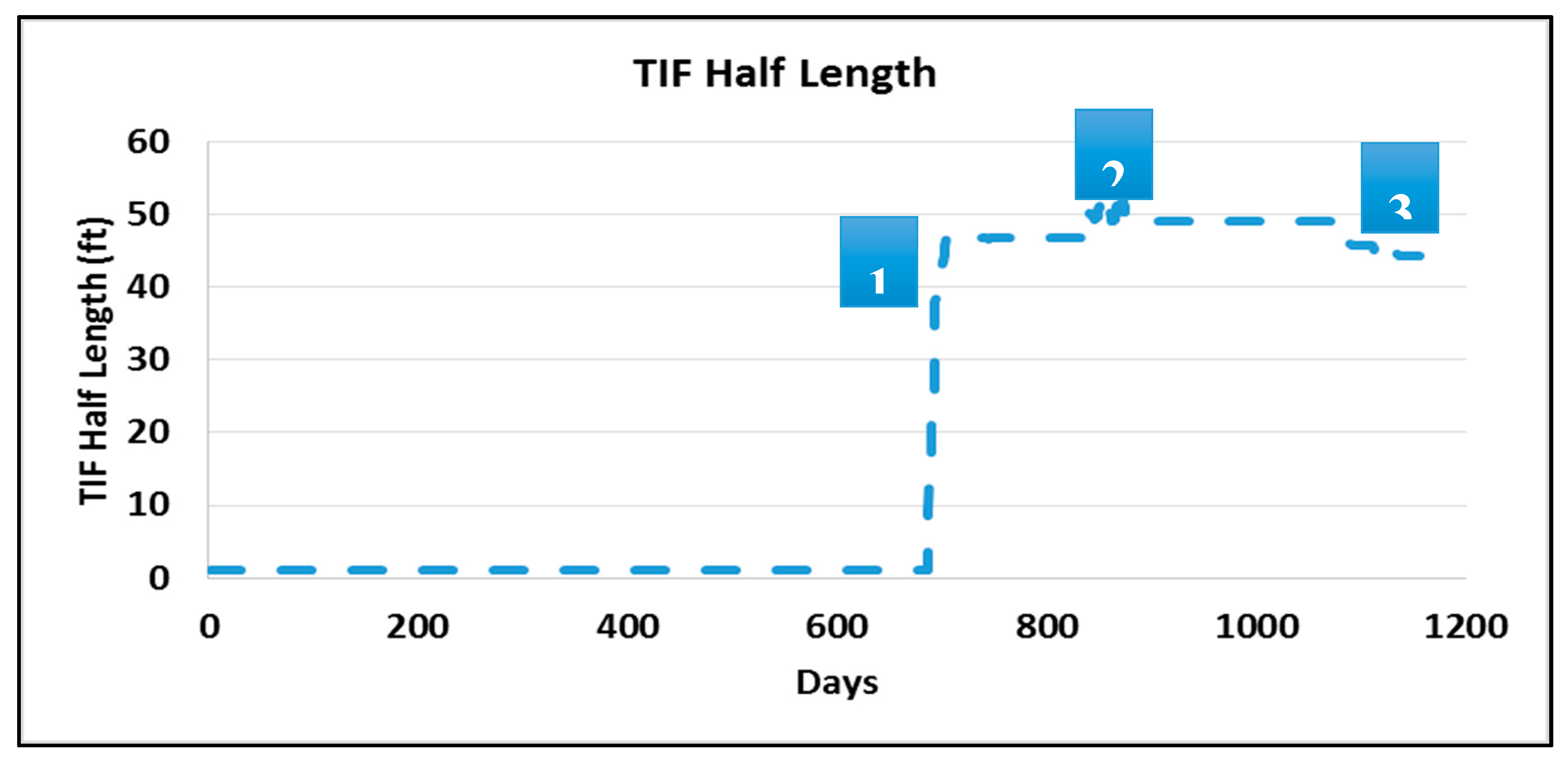
12.3. TIF Growth Dynamics
13. Conclusions
- The direction of maximum horizontal stress, and TIF propagation was most likely E–W, with a normal faulting regime.
- The surface water temperature and both the volume of the injected water and TIF propagation, were well-correlated, especially after the onset of the TIF at 690 days.
- History matching with TIF modelling proved to be time-consuming, due to the dynamic nature of TIFs and the presence of geomechanical uncertainties.
- Two workflows were developed for history matching for Well NI6 data. The reservoir and well parameters were first matched to the field data prior to TIF initiation at 690 days. The geomechanical properties were adjusted by history matching the subsequent field data to the TIF model.
- The model results without TIF were matched to the NI6 injection rate data before day 690. Inclusion of the TIF and suitable modifications to the initially estimated values of the geomechanical properties were required to obtain a comparable match after this date.
- The reservoir and geomechanical models were improved and validated once the modelled and observed TIF onset and propagation periods were confirmed
- The resulting history-matched N Field sector model can be used with confidence in future studies.
Funding
Acknowledgments
Conflicts of Interest
Appendix A
Appendix A.1. PVT Tables for the Thermal Model

| Temperature = 224.6 °F | ||||||||
|---|---|---|---|---|---|---|---|---|
| Pressure (psi) | Bubble Point (psi) | Gas Oil Ratio (scf/STB) | Oil FVF RB/STB | Oil Viscosity cp | Gas FVF (RB/Mscf) | Gas Viscosity (cp) | Water FVF RB/STB | Water Viscosity (cp) |
| 7251.89 | 738.415 | 1380.21 | 1.75093 | 0.283276 | 0.561812 | 0.033579 | 1.02306 | 0.32758 |
| 6890.03 | 738.415 | 1298.85 | 1.71203 | 0.292091 | 0.575612 | 0.032602 | 1.02428 | 0.32758 |
| 6528.16 | 738.415 | 1218.28 | 1.67351 | 0.303124 | 0.591175 | 0.031596 | 1.02551 | 0.32758 |
| 6166.31 | 738.415 | 1138.54 | 1.6354 | 0.316543 | 0.608871 | 0.030559 | 1.02673 | 0.32758 |
| 5804.45 | 738.415 | 1059.68 | 1.59769 | 0.332554 | 0.629183 | 0.029492 | 1.02795 | 0.32758 |
| 5442.58 | 738.415 | 981.727 | 1.56043 | 0.351413 | 0.652742 | 0.028393 | 1.02918 | 0.32758 |
| 5080.73 | 738.415 | 904.74 | 1.52362 | 0.37342 | 0.680391 | 0.027263 | 1.0304 | 0.32758 |
| 4718.88 | 738.415 | 828.775 | 1.4873 | 0.39893 | 0.71327 | 0.026103 | 1.03162 | 0.32758 |
| 4357.01 | 738.415 | 753.888 | 1.4515 | 0.428355 | 0.752957 | 0.024915 | 1.03284 | 0.32758 |
| 3995.15 | 738.415 | 680.158 | 1.41625 | 0.462165 | 0.801682 | 0.023706 | 1.03407 | 0.32758 |
| 3633.29 | 738.415 | 607.668 | 1.3816 | 0.500895 | 0.862681 | 0.022481 | 1.03529 | 0.32758 |
| 3271.43 | 738.415 | 536.518 | 1.34758 | 0.545137 | 0.940758 | 0.021254 | 1.03651 | 0.32758 |
| 2909.57 | 738.415 | 466.826 | 1.31427 | 0.59555 | 1.0433 | 0.020038 | 1.03774 | 0.32758 |
| 2547.71 | 738.415 | 398.739 | 1.28172 | 0.652833 | 1.18201 | 0.018856 | 1.03896 | 0.32758 |
| 2185.85 | 738.415 | 332.446 | 1.25002 | 0.717708 | 1.37632 | 0.017734 | 1.04018 | 0.32758 |
| 1823.99 | 738.415 | 268.179 | 1.2193 | 0.790879 | 1.66066 | 0.016701 | 1.0414 | 0.32758 |
| 1462.13 | 738.415 | 206.266 | 1.1897 | 0.872922 | 2.10233 | 0.015784 | 1.04263 | 0.32758 |
| 1100.27 | 738.415 | 147.181 | 1.16145 | 0.964077 | 2.85516 | 0.015003 | 1.04385 | 0.32758 |
| 738.415 | 738.415 | 91.6773 | 1.13492 | 1.06374 | 4.37215 | 0.014371 | 1.04507 | 0.32758 |
| 376.556 | 738.415 | 41.2191 | 1.1108 | 1.16895 | 8.84523 | 0.013896 | 1.04629 | 0.32758 |
| Temperature = 200 °F | ||||||||
|---|---|---|---|---|---|---|---|---|
| Pressure (psi) | Bubble Point (psi) | Gas Oil Ratio (scf/STB) | Oil FVF RB/STB | Oil Viscosity cp | Gas FVF (RB/Mscf) | Gas Viscosity (cp) | Water FVF RB/STB | Water Viscosity (cp) |
| 7251.89 | 738.415 | 1440.14 | 1.76358 | 0.323065 | 0.541712 | 0.0347134 | 1.01363 | 0.385872 |
| 6890.03 | 738.415 | 1355.25 | 1.72314 | 0.332854 | 0.554152 | 0.0337032 | 1.01479 | 0.385872 |
| 6528.16 | 738.415 | 1271.18 | 1.68309 | 0.345409 | 0.56817 | 0.0326593 | 1.01594 | 0.385872 |
| 6166.31 | 738.415 | 1187.99 | 1.64345 | 0.360948 | 0.584105 | 0.0315799 | 1.0171 | 0.385872 |
| 5804.45 | 738.415 | 1105.69 | 1.60425 | 0.379753 | 0.602395 | 0.0304631 | 1.01826 | 0.385872 |
| 5442.58 | 738.415 | 1024.36 | 1.5655 | 0.402172 | 0.623621 | 0.0293072 | 1.01942 | 0.385872 |
| 5080.73 | 738.415 | 944.029 | 1.52723 | 0.428631 | 0.64856 | 0.0281115 | 1.02058 | 0.385872 |
| 4718.88 | 738.415 | 864.763 | 1.48946 | 0.459644 | 0.678268 | 0.026876 | 1.02174 | 0.385872 |
| 4357.01 | 738.415 | 786.625 | 1.45224 | 0.495816 | 0.714225 | 0.0256024 | 1.0229 | 0.385872 |
| 3995.15 | 738.415 | 709.69 | 1.41559 | 0.537869 | 0.758529 | 0.0242948 | 1.02406 | 0.385872 |
| 3633.29 | 738.415 | 634.051 | 1.37955 | 0.586643 | 0.814251 | 0.0229603 | 1.02521 | 0.385872 |
| 3271.43 | 738.415 | 559.815 | 1.34418 | 0.643115 | 0.885996 | 0.021611 | 1.02637 | 0.385872 |
| 2909.57 | 738.415 | 487.097 | 1.30954 | 0.70842 | 0.980903 | 0.0202646 | 1.02753 | 0.385872 |
| 2547.71 | 738.415 | 416.054 | 1.27569 | 0.783847 | 1.11039 | 0.0189464 | 1.02869 | 0.385872 |
| 2185.85 | 738.415 | 346.882 | 1.24274 | 0.870853 | 1.29349 | 0.0176894 | 1.02985 | 0.385872 |
| 1823.99 | 738.415 | 279.824 | 1.21079 | 0.971055 | 1.56384 | 0.0165314 | 1.03101 | 0.385872 |
| 1462.13 | 738.415 | 215.222 | 1.18001 | 1.08614 | 1.98678 | 0.0155082 | 1.03217 | 0.385872 |
| 1100.27 | 738.415 | 153.572 | 1.15064 | 1.21767 | 2.71092 | 0.0146453 | 1.03333 | 0.385872 |
| 738.415 | 738.415 | 95.6586 | 1.12305 | 1.36632 | 4.17292 | 0.0139545 | 1.03449 | 0.385872 |
| 376.556 | 738.415 | 43.009 | 1.09797 | 1.52938 | 8.48563 | 0.0134408 | 1.03564 | 0.385872 |
| Temperature = 160 °F | ||||||||
|---|---|---|---|---|---|---|---|---|
| Pressure (psi) | Bubble Point (psi) | Gas Oil Ratio (scf/STB) | Oil FVF RB/STB | Oil Viscosity cp | Gas FVF (RB/Mscf) | Gas Viscosity (cp) | Water FVF RB/STB | Water Viscosity (cp) |
| 7251.89 | 738.415 | 1554.35 | 1.79168 | 0.383065 | 0.510262 | 0.0370349 | 1.00017 | 0.445872 |
| 6890.03 | 738.415 | 1462.73 | 1.74827 | 0.392854 | 0.520536 | 0.0359781 | 1.00126 | 0.445872 |
| 6528.16 | 738.415 | 1371.99 | 1.70529 | 0.405409 | 0.53208 | 0.0348808 | 1.00234 | 0.445872 |
| 6166.31 | 738.415 | 1282.2 | 1.66275 | 0.420948 | 0.545171 | 0.0337392 | 1.00343 | 0.445872 |
| 5804.45 | 738.415 | 1193.38 | 1.62068 | 0.439753 | 0.560171 | 0.0325496 | 1.00451 | 0.445872 |
| 5442.58 | 738.415 | 1105.59 | 1.57909 | 0.462172 | 0.577559 | 0.0313077 | 1.0056 | 0.445872 |
| 5080.73 | 738.415 | 1018.89 | 1.53802 | 0.488631 | 0.59799 | 0.0300097 | 1.00668 | 0.445872 |
| 4718.88 | 738.415 | 933.341 | 1.49749 | 0.519644 | 0.622365 | 0.0286523 | 1.00777 | 0.445872 |
| 4357.01 | 738.415 | 849.007 | 1.45754 | 0.555816 | 0.65196 | 0.0272331 | 1.00886 | 0.445872 |
| 3995.15 | 738.415 | 765.976 | 1.4182 | 0.597869 | 0.688622 | 0.0257524 | 1.00994 | 0.445872 |
| 3633.29 | 738.415 | 684.339 | 1.37953 | 0.646643 | 0.735094 | 0.0242142 | 1.01103 | 0.445872 |
| 3271.43 | 738.415 | 604.211 | 1.34157 | 0.703115 | 0.795582 | 0.0226291 | 1.01211 | 0.445872 |
| 2909.57 | 738.415 | 525.726 | 1.30439 | 0.76842 | 0.876744 | 0.0210164 | 1.0132 | 0.445872 |
| 2547.71 | 738.415 | 449.049 | 1.26807 | 0.843847 | 0.989484 | 0.0194088 | 1.01428 | 0.445872 |
| 2185.85 | 738.415 | 374.391 | 1.2327 | 0.930853 | 1.15229 | 0.017854 | 1.01537 | 0.445872 |
| 1823.99 | 738.415 | 302.015 | 1.19841 | 1.03106 | 1.39796 | 0.0164135 | 1.01645 | 0.445872 |
| 1462.13 | 738.415 | 232.291 | 1.16538 | 1.14614 | 1.78928 | 0.0151494 | 1.01754 | 0.445872 |
| 1100.27 | 738.415 | 165.751 | 1.13386 | 1.27767 | 2.46659 | 0.0141042 | 1.01863 | 0.445872 |
| 738.415 | 738.415 | 103.244 | 1.10425 | 1.42632 | 3.83983 | 0.0132894 | 1.01971 | 0.445872 |
| 376.556 | 738.415 | 46.4198 | 1.07733 | 1.58938 | 7.89285 | 0.0126981 | 1.0208 | 0.445872 |
| Temperature = 100 °F | ||||||||
|---|---|---|---|---|---|---|---|---|
| Pressure (psi) | Bubble Point (psi) | Gas Oil Ratio (scf/STB) | Oil FVF RB/STB | Oil Viscosity cp | Gas FVF (RB/Mscf) | Gas Viscosity (cp) | Water FVF RB/STB | Water Viscosity (cp) |
| 7251.89 | 738.415 | 1778.87 | 1.85765 | 0.443065 | 0.466801 | 0.0419478 | 0.98456 | 0.505872 |
| 6890.03 | 738.415 | 1674.01 | 1.8084 | 0.452854 | 0.474114 | 0.0408453 | 0.985617 | 0.505872 |
| 6528.16 | 738.415 | 1570.17 | 1.75963 | 0.465409 | 0.482251 | 0.039696 | 0.986674 | 0.505872 |
| 6166.31 | 738.415 | 1467.4 | 1.71136 | 0.480948 | 0.491384 | 0.0384941 | 0.987732 | 0.505872 |
| 5804.45 | 738.415 | 1365.76 | 1.66362 | 0.499753 | 0.501744 | 0.0372327 | 0.988789 | 0.505872 |
| 5442.58 | 738.415 | 1265.29 | 1.61643 | 0.522172 | 0.513639 | 0.0359036 | 0.989846 | 0.505872 |
| 5080.73 | 738.415 | 1166.07 | 1.56983 | 0.548631 | 0.527494 | 0.0344971 | 0.990903 | 0.505872 |
| 4718.88 | 738.415 | 1068.15 | 1.52384 | 0.579644 | 0.543904 | 0.0330019 | 0.991961 | 0.505872 |
| 4357.01 | 738.415 | 971.642 | 1.47851 | 0.615816 | 0.563736 | 0.0314047 | 0.993018 | 0.505872 |
| 3995.15 | 738.415 | 876.614 | 1.43387 | 0.657869 | 0.588294 | 0.0296912 | 0.994075 | 0.505872 |
| 3633.29 | 738.415 | 783.187 | 1.38999 | 0.706643 | 0.619589 | 0.0278469 | 0.995132 | 0.505872 |
| 3271.43 | 738.415 | 691.485 | 1.34692 | 0.763115 | 0.660867 | 0.0258612 | 0.996189 | 0.505872 |
| 2909.57 | 738.415 | 601.665 | 1.30473 | 0.82842 | 0.71758 | 0.0237346 | 0.997247 | 0.505872 |
| 2547.71 | 738.415 | 513.912 | 1.26352 | 0.903847 | 0.799251 | 0.0214918 | 0.998304 | 0.505872 |
| 2185.85 | 738.415 | 428.47 | 1.22338 | 0.990853 | 0.923274 | 0.0191999 | 0.999361 | 0.505872 |
| 1823.99 | 738.415 | 345.64 | 1.18448 | 1.09106 | 1.12244 | 0.0169865 | 1.00042 | 0.505872 |
| 1462.13 | 738.415 | 265.844 | 1.147 | 1.20614 | 1.45951 | 0.01503 | 1.00148 | 0.505872 |
| 1100.27 | 738.415 | 189.693 | 1.11123 | 1.33767 | 2.06563 | 0.0134766 | 1.00253 | 0.505872 |
| 738.415 | 738.415 | 118.158 | 1.07763 | 1.48632 | 3.30934 | 0.0123491 | 1.00359 | 0.505872 |
| 376.556 | 738.415 | 53.1249 | 1.04709 | 1.64938 | 6.97785 | 0.0115842 | 1.00465 | 0.505872 |
| Temperature = 60 °F | ||||||||
|---|---|---|---|---|---|---|---|---|
| Pressure (psi) | Bubble Point (psi) | Gas Oil Ratio (scf/STB) | Oil FVF RB/STB | Oil Viscosity cp | Gas FVF (RB/Mscf) | Gas Viscosity (cp) | Water FVF RB/STB | Water Viscosity (cp) |
| 7251.89 | 738.415 | 1976.74 | 1.9232 | 0.533065 | 0.44059 | 0.0464462 | 0.977331 | 0.595872 |
| 6890.03 | 738.415 | 1860.21 | 1.86879 | 0.542854 | 0.446223 | 0.0453275 | 0.978429 | 0.595872 |
| 6528.16 | 738.415 | 1744.82 | 1.8149 | 0.555409 | 0.452422 | 0.0441619 | 0.979526 | 0.595872 |
| 6166.31 | 738.415 | 1630.63 | 1.76156 | 0.570948 | 0.459302 | 0.0429434 | 0.980625 | 0.595872 |
| 5804.45 | 738.415 | 1517.67 | 1.70881 | 0.589753 | 0.467007 | 0.0416641 | 0.981721 | 0.595872 |
| 5442.58 | 738.415 | 1406.03 | 1.65666 | 0.612172 | 0.475734 | 0.0403147 | 0.982818 | 0.595872 |
| 5080.73 | 738.415 | 1295.77 | 1.60517 | 0.638631 | 0.485747 | 0.0388834 | 0.983917 | 0.595872 |
| 4718.88 | 738.415 | 1186.97 | 1.55436 | 0.669644 | 0.497419 | 0.0373553 | 0.985013 | 0.595872 |
| 4357.01 | 738.415 | 1079.71 | 1.50427 | 0.705816 | 0.511304 | 0.0357113 | 0.986112 | 0.595872 |
| 3995.15 | 738.415 | 974.12 | 1.45496 | 0.747869 | 0.528228 | 0.0339266 | 0.987209 | 0.595872 |
| 3633.29 | 738.415 | 870.298 | 1.40645 | 0.796643 | 0.549515 | 0.0319688 | 0.988307 | 0.595872 |
| 3271.43 | 738.415 | 768.398 | 1.35888 | 0.853115 | 0.577382 | 0.029798 | 0.989404 | 0.595872 |
| 2909.57 | 738.415 | 668.583 | 1.31225 | 0.91842 | 0.615803 | 0.0273679 | 0.990503 | 0.595872 |
| 2547.71 | 738.415 | 571.075 | 1.26671 | 0.993847 | 0.67232 | 0.0246424 | 0.991599 | 0.595872 |
| 2185.85 | 738.415 | 476.13 | 1.22237 | 1.08085 | 0.762122 | 0.0216381 | 0.992698 | 0.595872 |
| 1823.99 | 738.415 | 384.086 | 1.17937 | 1.18106 | 0.917317 | 0.0185031 | 0.993795 | 0.595872 |
| 1462.13 | 738.415 | 295.415 | 1.13797 | 1.29614 | 1.20562 | 0.0155876 | 0.994893 | 0.595872 |
| 1100.27 | 738.415 | 210.792 | 1.09844 | 1.42767 | 1.76154 | 0.0133162 | 0.99599 | 0.595872 |
| 738.415 | 738.415 | 131.301 | 1.06132 | 1.57632 | 2.92463 | 0.0117981 | 0.997087 | 0.595872 |
| 376.556 | 738.415 | 59.0339 | 1.02757 | 1.73938 | 6.34382 | 0.0108503 | 0.998182 | 0.595872 |
Appendix A.2. Correlations Used to Convert the Isothermal Reservoir Model to the Thermal One
| Coefficient | γo ≤ 30° API | γo ≤ 30° API |
|---|---|---|
| A1 | 0.0362 | 0.0178 |
| A2 | 1.0937 | 1.187 |
| A3 | 25.724 | 23.931 |
| C1 | 4.68 × 10⁻⁴ | 4.67 × 10⁻⁴ |
| C2 | 1.75 × 10⁻⁵ | 1.10 × 10⁻⁵ |
| C3 | −1.81 × 10⁻⁸ | 1.38 × 10⁻⁹ |
- = Oil formation volume factor (FVF)
- = Bubble point oil FVF
- = The solution Gas Oil Ratio (GOR)
- = The oil gravity, API
- = The gas gravity, (air = 1)
- = The bubble point pressure.
References
- Charlez, P.; Lemonnier, P.; Ruffet, C.; Bouteca, M.J.; Tan, C. Thermally Induced Fracturing: Analysis of a Field Case in North Sea. In Proceedings of the European Petroleum Conference, Milan, Italy, 22–24 October 1996. [Google Scholar]
- Suri, A.; Sharma, M.M. Fracture Growth in Horizontal Injectors. In Proceedings of the SPE Hydraulic Fracturing Technology Conference, The Woodlands, TX, USA, 19–21 January 2009. [Google Scholar]
- Svendson, A.P.; Wright, M.S.; Clifford, P.J.; Berry, P.J. Thermally Induced Fracturing of Ula Water Injectors. SPE Prod. J. 1991, 6, 384–390. [Google Scholar] [CrossRef]
- Petroleum Experts IPM 9.0. REVEAL Software Manual. Available online: https://www.scribd.com/document/328259134/Reveal-Complete (accessed on 5 January 2020).
- Detienne, J.L.; Creusot, M.; Kessler, N.; Sahuquet, B.; Bergerot, J.L. Thermally Induced Fractures: A Field-Proven Analytical Model. SPE Prod. Oper. J. 1998, 1, 30–35. [Google Scholar] [CrossRef]
- Settari, A.; Warren, G.M. Simulation and field analysis of waterflood induced fracturing. In Proceedings of the Rock Mechanics in Petroleum Engineering, Delft, The Netherlands, 29–31 August 1994. [Google Scholar]
- Williams, D.B.; Sherrard, D.W.; Lin, C.Y. The Impacts on Waterflood Management of Inducing Fractures in Injection Wells in the Prudhoe Bay Oil Field. In Proceedings of the SPE California Regional Meeting, Ventura, CA, USA, 8–10 April 1987. [Google Scholar]
- Felippa, C. Stress-Strain Material Laws; University of Colorado at Boulder: Boulder, CO, USA, 2017. [Google Scholar]
- Wu, Y.; Taylor, J.M.; Frei-Pearson, A.; Bryant, S.L. Injection Induced Fracturing as a Necessary Evil in Geologic CO2 Sequestration. In Proceedings of the 49th U.S. Rock Mechanics/Geomechanics Symposium, San Francisco, CA, USA, 28 June–1 July 2015. [Google Scholar]
- Papamichos, E.; Malmanger, E.M. A Sand-Erosion Model for Volumetric Sand Predictions in a North Sea Reservoir. In Proceedings of the Latin American and Caribbean Petroleum Engineering Conference, Caracas, Venezuela, 21–23 April 1999. [Google Scholar]
- Risnes, R.; Bratli, R.K.; Horsrud, P. Sand stresses Around a Wellbore. SPE Soc. Pet. Eng. J. 1982, 22, 883–898. [Google Scholar] [CrossRef]
- Vaziri, H.; Allam, R.; Kidd, G.; Bennett, C.; Grose, T.; Robinson, P.; Malyn, J. Sanding: A Rigorous Examination of the Interplay Between Drawdown, Depletion, Start-up Frequency and Water Cut. In Proceedings of the SPE Annual Technical Conference and Exhibition, Houston, TX, USA, 26–29 September 2004. [Google Scholar]
- Tovar, J.J.; Navarro, W. The Impact of sandstone strength’s behaviour as a result of temperature changes in Water Injectors. In Proceedings of the Europec/EAGE Conference and Exhibition, Rome, Italy, 9–12 June 2008. [Google Scholar]
- Salamy, S.P.; Al-Mubarak, H.K.; Al-Ghamdi, M.S.; Hembling, D.E. Maximum-Reservoir-Contact-Wells Performance Update: Shaybah Field, Saudi Arabia. SPE Prod. Oper. J. 2008, 23, 439–443. [Google Scholar] [CrossRef]
- Navarro, W. Produced Water Reinjection in Mature Field with High Water Cut. In Proceedings of the Latin American & Caribbean Petroleum Engineering Conference, Buenos Aires, Argentina, 15–18 April 2007. [Google Scholar]
- Ertekin, T.; Abou-Kassem, J.H.; King, G.R. Basic Applied Reservoir Simulation; SPE: Richardson, TX, USA, 2001; pp. 350–356. [Google Scholar]
- History Matching/Prediction. Presentations at New Mexico Institute of Mining and Technology. Available online: http://infohost.nmt.edu/~petro/faculty/Engler571/HistoryMatching.pdf (accessed on 9 April 2017).
- Perkins, T.K.; Gonzalez, J.A. Changes in Earth Stresses around a Wellbore Caused by Radially Symmetrical Pressure and Temperature Gradients. Soc. Pet. Eng. J. 1984, 24, 129–140. [Google Scholar] [CrossRef]
- Almarri, M.; Prakasa, B.; Muradov, K.; Davies, D. Identification and Characterization of Thermally Induced Fractures Using Modern Analytical Techniques. In Proceedings of the SPE Kingdom of Saudi Arabia Annual Technical Symposium and Exhibition, Dammam, Saudi Arabia, 24–27 April 2017. [Google Scholar]
- Clifford, P.J.; Berry, P.J.; Gu, H. Modeling the Vertical Confinement of Injection-well Thermal Fractures. SPE Prod. Eng. J. 1991, 6, 377–383. [Google Scholar] [CrossRef]
- Yew, C.H. Mechanics of Hydraulic Fracturing; Elsevier Science & Technology: Amsterdam, The Netherlands, 1997; pp. 30–34. [Google Scholar]
- Clifton, R.J.; Wang, J.J. Multiple Fluids, Proppant Transport, and Thermal Effects in Three-Dimensional Simulation of Hydraulic Fracturing. In Proceedings of the SPE Annual Technical Conference and Exhibition, Houston, TX, USA, 2–5 October 1988. [Google Scholar]
- Clifton, R.J.; Abou-Sayed, A.S. On the Computation of the Three-Dimensional Geometry of Hydraulic Fractures. In Proceedings of the Symposium on Low Permeability Gas Reservoirs, Denver, CO, USA, 20–22 May 1979. [Google Scholar]
- Clifton, R.J.; Abou-Sayed, A.S. A Variational Approach to the Prediction of the Three-Dimensional Geometry of Hydraulic Fractures. In Proceedings of the SPE/DOE Low Permeability Gas Reservoirs Symposium, Denver, CO, USA, 27–29 May 1981. [Google Scholar]
- Koning, E.J.L. Fractured Water Injection Wells—Analytical Modelling of Fracture Propagation. SPE Tech. J. 1985. Available online: https://www.onepetro.org/general/SPE-14684-MS (accessed on 20 April 2020).
- Perkins, T.K.; Gonzalez, J.A. The Effect of Thermoelastic Stresses on Injection Well Fracturing. Soc. Pet. Eng. J. 1985, 25, 78–88. [Google Scholar] [CrossRef]
- Hsiao, C.; Rabaa, A.W. Fracture Toughness Testing of Rock Cores. In Proceedings of the 28th U.S. Symposium on Rock Mechanics (USRMS), Tucson, AZ, USA, 29 June–1 July 1987. [Google Scholar]
- Roegiers, J.-C.; Zhao, X.L. The Measurement of Fracture Toughness of Rocks Under Simulated Downhole Conditions. In Proceedings of the 7th ISRM Congress, Aachen, Germany, 16–20 September 1991. [Google Scholar]
- Vazquez, M.; Beggs, H.D. Correlations for Fluid Physical Property Prediction. SPE J. Pet. Technol. 1980, 32, 968–970. [Google Scholar] [CrossRef]
- Oyeneyin, B. Integrated Sand Management for Effective Hydrocarbon Flow Assurance; Elsevier Science & Technology: Amsterdam, The Netherlands, 2015; pp. 133–160. [Google Scholar]
- Zoback, M.D.; Barton, C.A.; Brudy, M.; Castillo, D.A.; Finkbeiner, T.; Grollimund, B.R.; Moos, D.B.; Peska, P.; Ward, C.D.; Wiprut, D.J. Determination of stress orientation and magnitude in deep wells. Int. J. Rock Mech. Min. Sci. 2003, 40, 1049–1076. [Google Scholar] [CrossRef]
- Luo, X.; Were, P.; Liu, J.; Hou, Z. Estimation of Biot’s effective stress coefficient from well logs. Environ. Earth Sci. J. 2015, 73, 7019–7028. [Google Scholar] [CrossRef]
- Zhixi, C.; Mian, C.; Yan, J.; Rongzun, H. Determination of rock fracture toughness and its relationship with acoustic velocity. Int. J. Rock Mech. Min. Sci. 1997, 34, 41–49. [Google Scholar] [CrossRef]
- Martins, J.P.; Murray, L.R.; Clifford, P.J.; McLelland, W.G.; Hanna, M.F.; Sharp, J.W. Produced-Water Reinjection and Fracturing in Prudhoe Bay. SPE Reserv. Eng. J. 1995, 10, 176–182. [Google Scholar] [CrossRef]


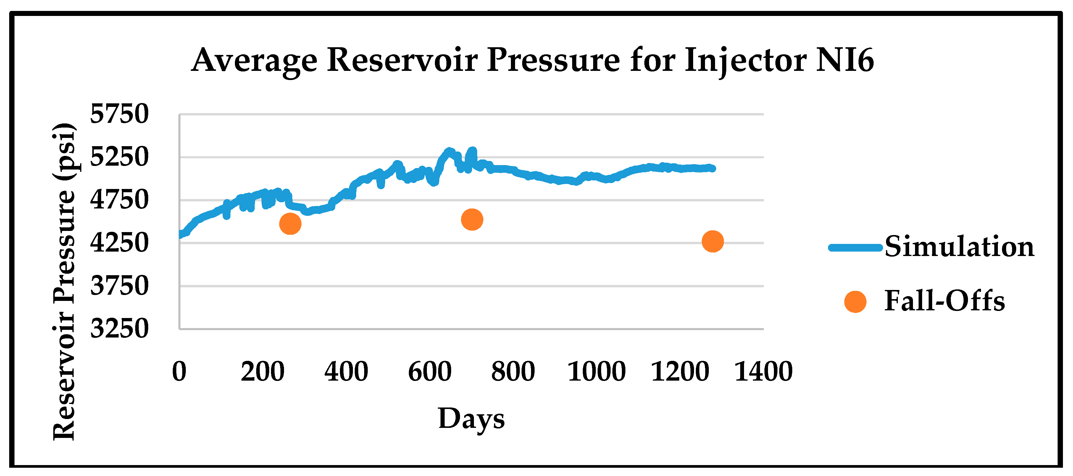


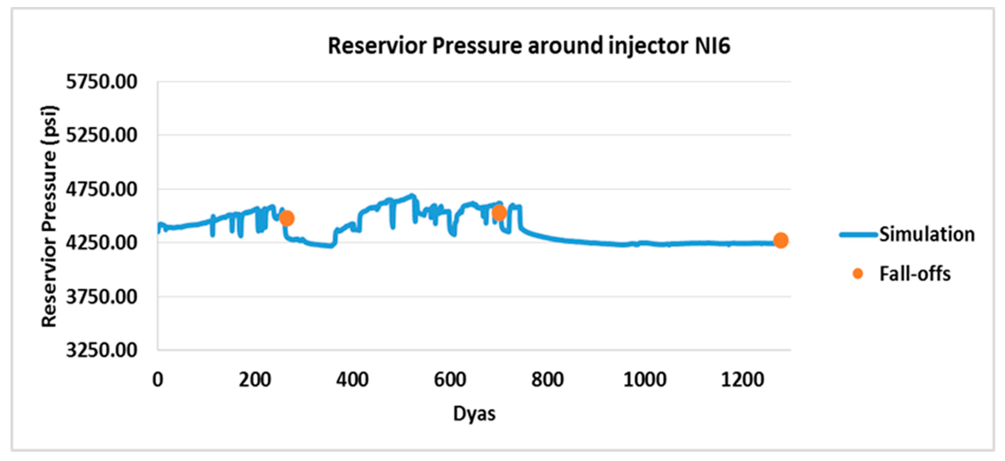

| Well NI6 Shutdowns | Average Regional Pressure (psi) | |
|---|---|---|
| After 266 days | July -09 | 4480.5 |
| After 702 days | Oct -10 | 4524 |
| After 1277 days | May -12 | 4263 |
| Test Points | Time (min) | Liquid Rate (STB/d) | ||
|---|---|---|---|---|
| Measured Values | Calculated Values | % Difference | ||
| Point 1 | 60.3 | 10,860 | 10,409 | −4.33 |
| Point 2 | 133.6 | 5013 | 5045 | 0.63 |
| Point 3 | 178.2 | 19,215 | 17,968 | −6.94 |
| Property Type | Property Name | Initial | Matched |
|---|---|---|---|
| Rock Mechanical Properties | Young’s modulus (MMpsi) | 6.8 | 2 |
| Poisson’s ratio | 0.23 | 0.35 | |
| Fracture toughness (psi/ft1/2) | 330.48 | 150 | |
| Biot’s coefficient | 0.53 | 0.67 | |
| In Situ Stresses | σv (psi/ft) | 0.97 | 0.97 |
| σHmax (psi/ft) | 0.86 | 0.86 | |
| σhmin (psi/ft) | 0.73 | 0.65 | |
| Thermal Property | Rock thermal expansion coefficient (1/F0) | 3.20 × 10⁻⁴ | 1.20 × 10⁻⁵ |
© 2020 by the author. Licensee MDPI, Basel, Switzerland. This article is an open access article distributed under the terms and conditions of the Creative Commons Attribution (CC BY) license (http://creativecommons.org/licenses/by/4.0/).
Share and Cite
Almarri, M. Efficient History Matching of Thermally Induced Fractures Using Coupled Geomechanics and Reservoir Simulation. Energies 2020, 13, 3001. https://doi.org/10.3390/en13113001
Almarri M. Efficient History Matching of Thermally Induced Fractures Using Coupled Geomechanics and Reservoir Simulation. Energies. 2020; 13(11):3001. https://doi.org/10.3390/en13113001
Chicago/Turabian StyleAlmarri, Misfer. 2020. "Efficient History Matching of Thermally Induced Fractures Using Coupled Geomechanics and Reservoir Simulation" Energies 13, no. 11: 3001. https://doi.org/10.3390/en13113001
APA StyleAlmarri, M. (2020). Efficient History Matching of Thermally Induced Fractures Using Coupled Geomechanics and Reservoir Simulation. Energies, 13(11), 3001. https://doi.org/10.3390/en13113001