Abstract
Under the influence of the COVID-19 pandemic and the concurrent oil conflict between Russia and Saudi Arabia, oil prices have exhibited unusual and sudden changes. For this reason, the volatilities of the West Texas Intermediate (WTI), Brent and Dubai crude daily oil price data between 29 May 2006 and 31 March 2020 are analysed. Firstly, the presence of chaotic and nonlinear behaviour in the oil prices during the pandemic and the concurrent conflict is investigated by using the Shanon Entropy and Lyapunov exponent tests. The tests show that the oil prices exhibit chaotic behavior. Additionally, the current paper proposes a new hybrid modelling technique derived from the LSTARGARCH (Logistic Smooth Transition Autoregressive Generalised Autoregressive Conditional Heteroskedasticity) model and LSTM (long-short term memory) method to analyse the volatility of oil prices. In the proposed LSTARGARCHLSTM method, GARCH modelling is applied to the crude oil prices in two regimes, where regime transitions are governed with an LSTAR-type smooth transition in both the conditional mean and the conditional variance. Separating the data into two regimes allows the efficient LSTM forecaster to adapt to and exploit the different statistical characteristics and ARCH and GARCH effects in each of the two regimes and yield better prediction performance over the case of its application to all the data. A comparison of our proposed method with the GARCH and LSTARGARCH methods for crude oil price data reveals that our proposed method achieves improved forecasting performance over the others in terms of RMSE (Root Mean Square Error) and MAE (Mean Absolute Error) in the face of the chaotic structure of oil prices.
1. Introduction
The petroleum market is currently going through one of the most volatile times in its history. The volatilities of crude oil prices are affected not only by macroeconomic and microeconomic variables but also by the speculative activities and non-economic variables such as geopolitical tensions, the Gulf war, and, nowadays, the coronavirus disease 2019 (COVID-19) and the conflict between Russia and Saudi Arabia. In the recent months, uncertainty and volatility in oil prices due to COVID-19 and the conflict between Russia and Saudi Arabia have impacted the investors’ decisions for portfolio allocation and manufacturers’ decisions for industrial production and economy. While the COVID-19 pandemic has led to worldwide recession, it has also resulted in a drop in demand for oil. The countries in the Middle East and North Africa (MENA) have been faced with both the COVID-19 pandemic as well as the steep decline in oil prices. That is, the petroleum market has endured the pressure of an increase in supply alongside a decrease in demand. In this respect, the differences in opinion between Russia and Saudi Arabia (on 9 April, Russia and Saudi Arabia resolved their opinion differences) and the disagreements among OPEC and countries on petroleum production reduction had an effect on the increase in supply.
Under the influence of COVID-19 and the conflict between Russia and Saudi Arabia, the petroleum market faced both a negative demand shock and a negative supply shock [1]. A negative supply shock arises from a drop in the workforce, which in the case of COVID-19 may be directly due to the workers acquiring the disease or may be indirect due to travel restrictions, lockdown conditions or tending to children staying at home. The supply is influenced by a drop in materials, capital and intermediate inputs due to the disturbances in the transportation network and admistration in MENA countries [2]. Negative demand shock exhibits global and local features [3]. Since the COVID-19 pandemic has caused recessions in all economies, the recessions, lockdown conditions, and disruptions to global value chains have resulted in a reduction in petroleum demand. It has shuttered factories; stopped people from travelling; increased the number of people staying at home; caused a drop in materials, capital and intermediate inputs due to the disturbances in the transportation network and admistration; and decreased production in many industrialised countries. That is, due to the restrictions in 187 countries and regions, petroleum demand has nearly stopped. The International Energy Agency (IEA) [4] has predicted that the petroleum demand will be 29 million barrels (mb/day) less in the month of April compared to in the same month a year ago. Moreover, this level is the lowest since 1995. For the second quarter of 2020, it is predicted that the demand will be 23.1 mb/day below the previous year’s demand.
Moreover, as mentioned above, together with the decline in petroleum demand, the petroleum supply, which maintained its pre-pandemic level, is responsible for the drop in petroleum prices. The petroleum storage capacities of countries have been filled for the first time in history [5]. On the other hand, to maintain market share, some oil producers stored their excess oil at sea by leasing tankers at high costs. As a consequence, the petroleum supply had to come down to the record low level of 12 mb/day in May. In future prices, West Texas Intermediate (WTI) entered the negative region and finished the day at the USD 37 per-barrel level.
Due to these unforeseen circumstances, the Middle East region is going through an unexpected turning point. Especially, the MENA countries are going through an economic recession triggered by the shock from COVID-19 [6], the breakdown in negotiations between the OPEC countries [5], the oil war between Russian and Saudi Arabia, and the uncertainties about China’s economic recovery. The economies of Saudi Arabia and Russia depend heavily on their oil revenues. Although the Russian economy is more diversified than Saudi Arabia’s economy, both economies face similar disruptions because oil revenues represent a very high share of their gross domestic products (GDPs). According to Kubursi [5], while Saudi Arabia needs a USD 80 per-barrel price to balance its budget, Russia needs a price of USD 60 to balance its government budget.
As the volatility of oil prices continues to increase, many countries and sectors will be affected. In this context, the volatility of oil prices points to both the regime models and the presence of a nonlinear and chaotic structure.
This paper aims to analyse the volatilities of WTI, Brent and Dubai crude oil prices between 29 May 2006 and 31 March 2020. Firstly, it explores the presence of chaotic and nonlinear behaviour in the oil prices by Shanon Entropy (SE) and Lyapunov exponent (Le) tests, and secondly, it suggests the Logistic Smooth Transition Autoregressive Generalised Autoregressive Conditional Heteroskedasticity long-short term memory (LSTARGARCHLSTM) method. If the SE and (Le) tests determine chaotic or nonlinear behavior, we propose a hybrid modelling technique developed by combining the LSTARGARCH [7] with LSTM. The LSTARGARCH model has STAR type nonlinearity in both the conditional mean and variance and allows the smooth transitions between the regimes to be governed by a logistic function. To evaluate the success or accuracy of our proposed method, we compare with GARCHLSTM and traditional methods; GARCH and LSTARGARCH. Finally, in this paper, since forecasting performance is accepted as a measure of the success of applied methods, we compare the forcasting performance of all the models.
This paper contributes to the related literature on theory, methodology and econometric applications by determining the differentiating characteristics of the volatility of the oil price in different regimes and by helping to specify the corresponding policies for these characteristics.
2. Related Work
Since the shocks stemming from COVID-19 have dramatically affected countries and many sectors, the impacts of the COVID-19 pandemic on the economy have been discussed by several papers. Baldwin [8] explored the connection between the inequality of wealth and health and the pandemic and argued that since for millions without higher education, financial and health difficulties abound, the number of hospitalisations and thereby the mortality rate due to COVID-19 is likely to be substantially higher for this group relative to that for the rest of the society. Gourinchas [9] pointed out that flattening the pandemic curve inevitably makes the macroeconomic recession curve steeper, which can be flattened by taking appropriate economic measures at a fiscal cost. Gopinath [10] discussed limiting the economic fallout from the coronavirus with targeted policies. Blanchard [11] and Alesina and Giavazzi [12] focused on ways to avoid another Euro crisis due to COVID-19. Gali [13] showed the importance of “helicopter money”, suggested by Gali [14] to avoid recession. Wyplosz [15] presented a solution to avoid a potential debt crisis during COVID-19. Cecchetti and Schoenholtz [16] accented the importance of Bank Runs and Panics. Cochrane [17] explored the impact of COVID-19 on monetary policy. Bénassy-Quéré [18] accented that the decline in oil prices will impact headline inflation and, as occurred in the past, could impact household and corporate inflation expectations. Arezki et al. [2,3] stressed that to limit the risk of financial instability, interest rates should be reduced and liquidity should be injected into the banking system and accented that, in places where inflation is low, liquidity injection and targeted cash transfers can be financed by “helicopter money” [14] that is banknotes printed by the central banks [13].
However, these studies do not consider the impacts of COVID-19 on the volatilities of oil prices, which has caused many issues. In our opinion, the volatility of oil prices points to both the regime structure and the presence of nonlinear and chaotic structure. Some previous work examined the volatility of the oil price and modelled it as a process with chaotic and nonlinear behavior. Barone-Adesi et al. [19] suggested a semiparametric method to examine the structure of oil prices. Adrangi et al. [20] determined the presence of low-dimensional chaotic structure in the oil prices. Lahmiri [21], Komijani et al. [22] and He [23] are the other studies that determine the presence of chaos in oil prices.
On the other hand, some previous studies emphasised the presence of outliers in the oil price. The outliers may impact the estimation and identification power of the generalised autoregressive conditional heteroskedasticity (GARCH) methods and can cause heteroscedasticity or conditional heteroscedasticity [24,25]. Moreover, they can affect the out-of-sample forecasting performance [24,26]. To address the issue of outliers, different methods have been proposed. Ané et al. [27] tested the performance of a method after noticing the outliers in a GARCH model by employing their proposed method. Charles and Darné [28] detected and corrected the outliers in the GARCH models. However, these methods do not have high forecasting performance.
Some papers combined STAR (Smooth Transition Autoregressive) and GARCH methods to reduce the problems mentioned above. The STAR technique by Teräsvirta [29], Luukkonen et al. [30] and Granger and Teräsvirta [31] suggest the nonlinear approach of the conditional mean based on smooth transition between stages of autoregressive processes by using the exponential and logistic squashing functions. Following these studies, González-Rivera [32], Hagerud [33], Dufrénot et al. [34] and Anderson et al. [35] suggested the STARGARCH (STGARCH) model, and Ané and Ureche-Rangau [36] suggested the Regime Switching Asymmetric Power GARCH (RS-APGARCH) model. Franses et al. [37] emphasised the importance of the STARGARCH methods. Lundbergh et al. [38] employed a STARGARCH method that permits non-linearity in both the conditional variance and the conditional mean. Lee and Degennaro [39], Chan and McAleer [40] showed the statistical properties of STARGARCH models. Bildirici and Ersin [41] suggested the STARSTGARCH model.
Some papers used various methods based on econometric models or intelligent algorithms such as Neural Network [42,43,44,45,46,47], genetic algorithms (GA) [48], support vector machines (SVM) [49] and support vector regression improved with a meta-heuristic algorithm [50,51]. The other studies in the literature adopted a decomposition-integration (EMD) method. Zhang et al. [52] and Yu et al. [53] used the EMD method to determine the main driving power behind the volatility of oil prices and showed that irregular events increase volatility.
Donaldson and Kamstra [42] suggested a class of Neural Network GARCH models. Gonzalez Miranda and Burgess [43], Hamid and Iqbal [44], and Bildirici and Ersin [45] combined the neural network method with the GARCH model to predict oil prices. Roh [47] combined the EWMA, GARCH and EGARCH models with a feedforward neural network model and determined that the EGARCH model with the feedforward neural network gives the best results. Kristjanpoller and Hernández [54] compared the predictability with a GARCH model against that with a hybrid neural network (HNN) and argued that, for forecasting volatility, HNN models are more suitable than the GARCH models.
A few papers analysed oil price volatility by combining regime models and neural network methods. Bildirici and Ersin [7] used the LSTARLSTGARCH family and LSTARLSTGARCHNN family to analyse oil prices. According to results of this work, the volatility, nonlinearity and asymmetric characteristics of oil prices were best captured by the LSTARLSTGARCHMLP family models. Bildirici and Ersin [55] suggested the LSTARLSTGARCHRBF models for forecasting the returns of oil prices. Their results indicated that the LSTARLSTGARCHRBF and LSTARLSTGARCHMLP models provide significant improvements over GARCH models.
On the other hand, some papers combined LSTM and GARCH models. Wex et al. [56] and Yu et al. [57] integrated financial news into the process of forecasting crude oil prices. Zhao et al. [58] used LSTM for oil price forecasting. Chen et al. [59] suggested the deep learning model to forecast oil prices. Gupta and Pandey [60] tested the volatility of oil prices by employing LSTM-based recurrent neural networks. For forecasting oil prices, Li et al. [61] suggested the EEMD-SBL-ADD method, which combines EEMD (ensemble empirical mode decomposition) and SBL (sparse Bayesian learning). Huang and Wu [62] used deep multiple kernel learning (DMKL) and showed that this method decreased the forecasting errors. Li et al. [63] suggested models based on deep learning to forecast oil prices where text and financial features were presented as complementary features for the deep learning models to obtain forecasts of oil prices with higher accuracy. Kim and Won [64] also proposed a hybrid model that combines the GARCH model with LSTM (long short-term memory) to forecast financial volatility. However, this work does not integrate deep learning with a regime switching GARCH method.
3. Methodology
In this paper, in accordance with Franses et al. [65], Terasvirta [66], and Chan and McAleer [67], STARGARCH type models are applied. The LSTARGARCH model supports STAR-type nonlinearity both in the conditional mean and in the conditional variance. In this model, the conditional volatility is based on the size and sign of the shocks on . Since the relative impacts of positive and negative shocks with equal magnitude depend on their conditional volatility, negative and positive shocks with similar sizes produce different effects [41,55].
Consider the following STAR model with two regimes:
where
It was defined with the logistic function. is the logistic transition function restricted to allow the transition to be a function of a single variable s and its respective distance to the threshold c.
takes positive values. When , it shows the TAR (threshold autoregressive) model. On the other hand when , the transition becomes smoother. If and , then . However, if , then . The function moves very quickly from 0 to 1. When the transition function is too steep, the LSTAR model converts to a SETAR (self exciting threshold autoregressive) model with two regimes. When , converges to a constant, and if , is equal to 0.5 and the LSTAR model turns into a linear AR(p) model.
The LSTARGARCH model is a model that allows STAR-type nonlinearity in both the conditional mean and the conditional variance. When the error terms follow a smooth transition in the GARCH process, by allowing GARCH errors, is obtained following equation:
The model is called STARGARCH. Since the information matrix of the STARGARCH Log-likelihood (LL) function is block diagonal, the parameters in the conditional mean equations can be estimated separately from the parameters in the conditional variance equations, as in the case of ARMA-GARCH.
To achieve a smooth transition in the GARCH procedure for the error terms and to obtain the LSTARGARCH model, the following equation is used:
The transition function is:
where n is the threshold coefficient and is the parameter defining the speed of the transition.
The Proposed Hybrid LSTARGARCHLSTM Model
LSTM is combined with GARCH methods (Figure 1) and LSTARGARCH (Figure 2) to gain assistance from the forecasting abilities of deep learning.
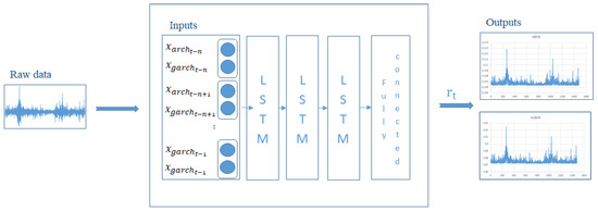
Figure 1.
Block diagram of the proposed GARCHLSTM method.
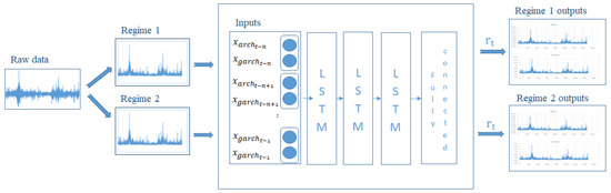
Figure 2.
Block diagram of the proposed LSTARGARCHLSTM method.
LSTM models have been proposed to exploit short- and long-term dependencies between the predicted time series data and the feature vectors extracted from it for performing the prediction. LSTM models were initially proposed in the seminal work of [68], which employed multiplicative gate units for maintaining a constant error flow through the constant error carousel unit to prevent the vanishing or blowing up of the error signals flowing backwards in time. A later variant of this fundamental architecture employed adaptive forget gates [69] to prevent the internal state from growing indefinitely by enabling the LSTM cell to learn to reset itself when its contents are outdated.
The equations governing the LSTM operation may be given as
where a is a bias vector, Q and V are weight matrices, the sigmoid function is denoted as σ(·), and denotes element-wise multiplication.
In the above, LSTM has a memory cell that has three gates. is the cell state vector. The activation vectors of the three gates are found according to Equations (8)–(10). In these equations, the weighted sum of input vector , the past output vector and the bias vector are passed through the sigmoid function to generate activation values in the range of 0 to 1. An activation value of one at each of these gates causes the information at the input to that gate to completely pass through, whereas a value of zero forces all the information at the input to be entirely filtered out. Hence, in Equation (6), the forget gate decides on the information in the most recent cell state () that passes to the current cell state. Similarly, in Equation (6), the input gate decides on the part of the new information to be stored in the current cell state (). Equation (7) computes the new information at time t as a weighted sum of , , and the bias where the output of the tanh activation function ranges between −1 and 1. Finally, the normalised output value in Equation (11) is determined by filtering the tanh normalised (range −1 to 1) cell state by using the output gate activation determined in Equation (10). This process separates the necessary information from unnecessary information to yield the output vector .
4. Data and Results
4.1. Data
We used Brent, Dubai and WTI crude oil price data in the current work. The volatilities of the Brent, Dubai and WTI crude oil prices are calculated by employing the daily closing prices between 29 May 2006 and 31 March 2020. lbopt, ldopt and lwopt show the volatilities of the Brent, Dubai and WTI crude oil prices, respectively. They were calculated as lbopt = ), ldopt = ) and lwopt = ).
In the process of the estimation of the GARCHLSTM and LSTARGARCHLSTM models, the sample is split between training, validation and out-of-sample elements in chronological order with respective proportions of 80%, 10% and 10%.
4.2. Results
The results were collected by the following five steps listed below:
- Firstly, some descriptive statistics were obtained. The Augmented Dickey-Fuller (ADF) unit root test [70,71] and Kapetanios, Shin, and Snell (KSS) unit root test [72] were applied. The ADF test is dependent upon a linear assumption that can cause the false results. Bigman et al. [73] showed that traditional unit root tests tends to produce “spurious regressions”. In this condition, for confirmation, we used the KSS test.
- Secondly, Tsay and Hsieh’s tests and the Brock–Dechert–Scheinkman (BDS) test were applied. These tests determined the presence of nonlinear structure, but they are not sufficient to determine the existence of chaotic behavior.
- Thirdly, SE and Le tests were applied. Le is a convenient means to decide on the presence of chaotic behavior.
- The LSTARGARCHLSTM method determines ARCH and GARCH effects. To evaluate the performance of our proposed method, we compared our proposed method with GARCHLSTM and traditional methods: GARCH and LSTARGARCH. For this purpose, GARCH and LSTARGARCH, and GARCHLSTM models were estimated and the most succesful model was determined.
- In the final step, the forecast accuracies of all of the models were determined.
4.2.1. Some Descriptive Statistics and Tsay and Hsieh’s Tests
In Table 1, several statistics of the data are shown. Since the data exhibit excess kurtosis, they cannot be modelled by a normal distribution. The normality assumption is rejected by the Jarque–Bera [74] (JB) normality test. The results show that nonnormality is observed and that normality is rejected.

Table 1.
Descriptive statistics and unit root tests. lbopt, ldopt and lwopt are the volatilities of the Brent, Dubai and WTI crude oil prices, respectively. ARCH shows the Engle’s [75] ARCH test statistic. White [76] shows White’s heteroscedasticity test statistic, RESET show the RESET statistic, and this test adds the second power of the fitted value as an additional regressor.
On the other hand, in Table 1, the main problem appears to be excess kurtosis but not excess skewness.
The ADF and KSS unit root tests suggest the stationarity of the data at the level. The KSS test implies that the data are nonlinear and stationary.
4.2.2. BDS Test, Tsay Tests and Hsieh’s Coefficients Results
The BDS test (for detailed knowledge, see Brock et.al. [77]) was developed to test whether the data generating process of a series is deterministic (chaotic) or not [78]. The BDS test does not have a simple interpretation because the result of this test determines whether the stochastic process has chaos or nonlinearity [79].
The BDS test can be used to determine the presence of nonlinearity in the time series. Hsieh [80] calculate the following BDS test statistic: Let be the fraction of the maximum norm of deviations of points in a time window of size m from points in a shifted time window of size m less than e. Under the null hypothesis of the time series , and for fixed m and e, , the BDS test statistic is the difference between and normalised by its standard deviation and asymptotically has the standard normal distribution. When the null hypothesis is rejected, nonlinear dynamics can be said to exist in the time series.The power of the test depends critically on the choice of e.
In Table 2, the BDS test determined that the lbopt, ldopt and lwopt variables indicate evidence of chaotic structure or nonlinear stochastic processes.
Table 2.
Brock–Dechert–Scheinkman (BDS) test results.
The Hsieh’s [81] coefficients are obtained in Table 3. Some coefficients are high. Although the Hsieh’s coefficients are not aimed at testing models that are nonlinear in variance, the high coefficient values indicate some autoregressive conditional heteroscedastic (ARCH) effects and other kinds of nonlinearities (such as GARCH-in-Mean effects).
Table 3.
Tsay test and Hsieh’s coefficients. rij’s are Hsieh’s [81] third-order moment coefficients. Hsieh’s [81] third-order moment coefficients were obtained as . Only coefficients for r(1, 1) and r(1, 2) were given.
Similarly, as shown in Table 3, the Tsay nonlinearity test determined that the linear form is misspecified for the op (oil price) variables. The RESET and Tsay nonlinearity test statistics do suggest that the (linear) functional form is misspecified for the variables.
4.2.3. Lyapunov Exponent and Kolmogorov Entropy Tests
The chaotic level of the time series can be measured with Le. Le is used to measure the average divergence from or convergence to the initial point of a dynamical system. If the Le has a large value, it indicates high sensivity to initial conditions. While a positive Lyapunov coefficient typically signifies chaotic structure, a negative coefficient typically shows convergence to initial conditions [21,82]. The positive value of Le indicates the presence of chaotic structure in the oil prices. Table 4 shows the results. Additionally, Adrangi and Chatrath [20], Bildirici and Sonustun [82], and Lahmiri [21] also determined the existence of chaotic structure for oil prices.
Table 4.
Lyapunov exponent and Shannon entropy results 1.
SE is applied to measure the randomness degree in the data. The SE is 0.9121 for lwopt. Entropy may be understood as the degree of the distortion of the market information reflected in the price system. Positive values of the entropy accent that the oil price information can still be used to understand the oil market dynamics. For example, since the reciprocal of the entropy for Brent is , the corresponding time scale of an effective and rational forecast for that entropy value must be within ~11 days. He [23] found 36 days by using the Kolmogorov entropy, and Bildirici [84] found 68 days.
4.2.4. Results with the GARCH, LSTARGARCH, LSTARGARCHLSTM and GARCHLSTM Models
Firstly, the results with the basic GARCH model and LSTARGARCH model are presented in Table 5. Statistical inference for assessing the empirical validity of the two regime switching process was carried out by using nonstandard Likelihood Ratio (LR) test [85]. However, these tests have some problems in the context of the LSTARGARCH method, since LSTARGARCH models support LSTAR-type nonlinearity in the conditional mean with GARCH-type heteroscedasticity in the conditional variance. We continue with LL test. There are two results: (1) the forms of the LL functions are obtained by the choice of the transition functions and (2) in the models, it can be possible to change the forms of the LL functions by transforming the parameters.
Table 5.
Baseline models. LogL: Log-likelihood, ARCH(p): pth order ARCH–LM test, AIC: Akaike information criterion, SIC: Schwarz information criterion, HQ: Hannan–Quinn information criterion.
Table 5 gives the results determined by traditional methods. LSTARGARCH models were employed to analyse the non–linearity in the conditional variance and in the conditional mean. When the two groups of results with the GARCH and LSTARGARCH models in Table 5 are compared, several conclusions can be derived. In the GARCH model, the sum of the ARCH and GARCH coefficients is in the range 0.8–0.9. The the sum of the coefficients of ARCH and GARCH is <1 but close to 1 for the LSTARGARCH method.
The results of LSTARGARCH model show significant improvements over the GARCH model. The Log-likelihood values are considerably smaller for LSTARGARCH method, and the Schwarz information criterion (SIC) and Akaike information criterion (AIC) are significantly lower. As shown by the results in Table 5, when the variance is not constant, the LSTARGARCH model can provide improvements in modelling.
4.2.5. The Architecture of the GARCH–LSTM and LSTARGARCH–LSTM Models
We will give the architecture of models with LSTM in Table 6. LSTM has been implemented in the Keras framework. The LSTM model is estimated with optimisation conducted simultaneously in the training and test samples. The optimisation is stopped at the epoch in which the test sample Mean Absolute Error (MAE) starts to increase while the training sample MAE continues to decrease (early stopping). The weight decay is also applied in the output and hidden layers to reduce overfitting. The LSTM network has been trained for 50 epochs by using approximately 80% of the data. Several models employing different numbers of layers of LSTM in a stack architecture have been evaluated by using the MAE measure on the validation error. The best model with the lowest MAE consisted of three LSTM layers (excluding the fully connected output layer). The selected methods are utilised for out-of-sample forecasting.
Table 6.
Generalised Autoregressive Conditional Heteroskedasticity long-short term memory (GARCHLSTM) and Logistic Smooth Transition Autoregressive (LSTAR) GARCHLSTM.
The determined models are used to forecast out-of-sample.
In our model, we use a stack of three LSTM layers followed by a fully connected layer at the output. A choice for the window size of 32 limits the support for the learning to the most recent 32 samples. The network is trained using an optimisation algorithm that adapts the parameter learning rate to both the first and second moments of the gradients to minimise the loss function. It can be shown as in Figure 1 and Figure 2.
4.2.6. The Results of the GARCHLSTM and LSTARGARCHLSTM Method
For comparative purposes, the results obtained by GARCHLSTM and our proposed methods are reported in Table 7. Our proposed method shows improvements over the LSTARGARCH model. The Log-likelihood value is decreased, and the SIC and AIC of our proposed method are lower than those of the LSTARGARCH model. Similarly, the results show improvements of the GARCHLSTM model in the GARCH models. The Log-likelihood values are decreased, and the SIC and AIC values are lower.
Table 7.
GARCHLSTM and LSTARGARCHLSTM. LogL: Log-likelihood, ARCH(p): pth order ARCH–LM test.
For the GARCHLSTM method and our proposed method, the stability conditions were realised. The Hannan–Quinn information criterion (HQ), SIC and AIC are are lower than for the GARCHLSTM. Moreover, after permitting the GARCH methods to follow LSTAR non–linearity, the dynamics are outstandingly different in terms of the estimated parameters.
5. Forecast Results
The forecast results are given under two subtitles: In–sample Forecast Results and Out of Sample Forecast Results.
5.1. In–Sample Forecast Results
In the in-sample forecast, the predictive capabilities of the models developed using observed data are formally evaluated to find out the effectiveness of the algorithms in reproducing data. The results show that our proposed method offers important advances in in-sample forecast accuracy (Table 8).
Table 8.
In-step forecast results.
In Table 7, forecasting performance results are presented. When the models are appraised in terms of the RMSE criterion, our proposed method has the highest forecasting power followed by the LSTARGARCH method. In terms of the RMSE criterion, the our proposed method has the best generalisation capability followed by the LSTARGARCH method.
5.2. Out-of-Sample Forecast Results
The models are obtained to explore their 1, 10 and 20 day-ahead forecast accuracies, shown in Table 9 (denoted as T + 1, T + 10 and T + 20). Accordingly, the out-of-sample 1, 10 and 20 days ahead forecasts with our proposed methods exhibited the lowest RMSE and MAE followed by those from the LSTARGARCH, GARCHLSTM and GARCH models.
Table 9.
Out of sample forecast results 1, 10 and 20 days ahead.
For example, for the WTI data, there is an order of magnitude improvement in the 10 and 20 days ahead forecast RMSE’s with the LSTARGARCH models when the models are augmented with the LSTM architecture. The RMSEs of our proposed methods for the WTI data in 1, 10 and 20 days are calculated as 0.0021, 0.0022 and 0.0025.
5.3. To Test for Forecast Accuracy
The Wilcoxon signed-rank (WS) and Diebold–Mariano (DM) tests were applied to confirm the equivalence of forecast accuracy [86]. The DM test is as follows:
where and is a consistent estimate of .
The results of these tests are presented in Table 10. The p-values for the DM test are given below the diagonal, and the p-values of the WS test are given above the diagonal. The H0 hypothesis of these tests assumes that the models have the same level of accuracy. For most cases, since the p-value is <0.05, the H0 hypothesis is rejected. For both tests, the p-value is >0.05 only for the RMSE comparison of the GARCH and GARCHLSTM models. Hence, these two models are comparable in terms of RMSE performance.
Table 10.
Wilcoxon signed-rank and Diebold–Mariano results.
6. Conclusions
This paper suggested a hybrid model for analysing oil price volatility between 29 May 2006 and 31 March 2020 on WTI, Brent and Dubai crude oil price datasets. Since under the influence of the COVID-19 pandemic and oil conflict between Russia and Saudi Arabia, the oil price has exhibited unusual changes, under the presence of chaotic structure of the oil price, analysis cannot be performed by traditional methods. The GARCH and LSTARGARCH methods and their extensions GARCHLSTM and LSTARGARCHLSTM based on deep learning were comparatively evaluated. The GARCH model may not achieve high forecasting performance under the presence of nonlinear or chaotic movement, since it considers the data period as a whole. Among these models, the LSTARGARCHLSTM model exhibited significantly better results in terms of out-of-sample accuracy than the others in the face of the chaotic structure of the oil price.
The LSTARGARCHLSTM model presents important improvements for time series estimation by dividing the data into regimes, and analysing each regime within itself with the effects of ARCH and GARCH. Specifically, the different GARCH and ARCH coefficients obtained in each of the negative and positive shocks show different ARCH and GARCH effects in each of the regimes and an obligation to set different policies in each of the regimes. According to our results, the impacts and the volatility of the oil shocks associated with COVID-19 must be evaluated by our proposed method.
According to the ARCH and GARCH coefficients of the LSTARGARCHLSTM methods, the oil price has ARCH and GARCH effects. That is, the oil supply and demand shocks associated with COVID-19 are likely to be short–lived, but their effects on many sectors and countries are persistent.
Oil demand and supply will get back to their pre-pandemic levels at a speed based on the length and depth of the disruption over time. Governments must develop policies to eliminate the adverse consequences of the supply and demand shocks caused by COVID-19. On the other hand, the COVID-19 pandemic will cause different results in oil-importing and -exporting countries. For oil-importing countries, the persistence of oil prices is important for determing policies for targeting inflation. Under the pressure on the prices of precious metals like gold and palladium, they can encounter problems related to policies of targeting inflation. The expectations have adverse effect and can produce unexpected results.
For oil-exporting countries, it is essential for Russia and OPEC countries to conduct policies to make the oil prices return to the levels before COVID-19, since oil revenues constitute a significant portion of the gross domestic products of these countries.
As accented by [2,3], in some oil-exporting and -importing countries, government coffers make the fight in containing the spread of COVID-19 and its economic and social impacts more difficult. Financial gaps in MENA countries as well as the high sovereign-risk premiums of many countries in the world present difficulties for additional foreign borrowing on private markets. For oil-importing and -exporting countries, helicopter money can be used as a recommended policy. However, fixed exchange rates in some countries may make it difficult for them to use helicopter money, since money printing is at odds with maintenance of the peg. As a result, in our opinion, if the oil prices do not return to the levels before the pandemic, oil-exporting countries will endure heavy losses.
Author Contributions
Conceptualization, formal analysis, methodology, investigation, software, writing—review and editing, M.B.; formal analysis, methodology, investigation, resources, software, writing—review and editing, N.G.B.; formal analysis, investigation, methodology, resources, writing—original draft, Y.U. All authors have read and agreed to the published version of the manuscript.
Funding
This research received no external funding.
Conflicts of Interest
In accordance with MDPI policy and our ethical obligation as a researcher, We have not any conflict of interest.
References
- Baldwin, R.; di Mauro, B.W. Mitigating the COVID Economic Crisis: Act Fast and Do Whatever; Baldwin, R., di Mauro, B.W., Eds.; CEPR Press: London, UK, 2020; pp. 1–24. [Google Scholar]
- Arezki, R.; Fan, R.Y.; Nguyen, H. Covid-19 and Oil Price Collapse: Coping with a Dual Shock in the Gulf Cooperation Council. ERF Policy Brief No. 52. April 2020. Available online: https://erf.org.eg/wp-content/uploads/2020/04/PB-52_Rabah_version3.pdf (accessed on 4 May 2020).
- Arezki, R.; Nguyen, H. Coping with a Dual Shock: COVID–19 and Oil Prices; World Bank: Washington, DC, USA, April 2020; Available online: https://www.worldbank.org/en/region/mena/brief/coping-with-a-dual-shock-coronavirus-covid-19-and-oil-prices (accessed on 4 May 2020).
- IEA. Oil Market Report—April (2020). Available online: https://www.iea.org/reports/oil–market–report–april–2020 (accessed on 4 May 2020).
- Kubursi, A. Oil Crash Explained: How Are Negative Oil Prices Even Possible? Available online: https://www.weforum.org/agenda/2020/04/negative–oil–prices–covid19/ (accessed on 4 May 2020).
- Soliman, M. COVID–19, the Oil Price War, and the Remaking of the Middle East. Available online: https://www.mei.edu/publications/covid–19–oil–price–war–and–remaking–middle–east (accessed on 4 May 2020).
- Bildirici, M.; Ersin, Ö.Ö. Forecasting oil prices: Smooth transition and neural network augmented GARCH family models. J. Pet. Sci. Eng. 2013, 109, 230–240. [Google Scholar] [CrossRef]
- Baldwin, R. The COVID–19 upheaval scenario: Inequality and pandemic make an explosive mix. VOX CEPR Policy Portal 2020. Available online: https://voxeu.org/article/inequality-and-pandemic-make-explosive-mix (accessed on 4 May 2020).
- Gourinchas, P.-O. Flattening the pandemic and recession curves. In Mitigating the COVID Economic Crisis: Act Fast and Do Whatever It Takes; Baldwin, R., di Mauro, B.W., Eds.; CEPR: London, UK, 2020; pp. 31–40. [Google Scholar]
- Gopinath, G. Limiting the economic fallout of the coronavirus with large targeted policies. In Mitigating the COVID Economic Crisis: Act Fast and Do Whatever; Baldwin, R., di Mauro, B.W., Eds.; CEPR: London, UK, 2020; pp. 41–48. [Google Scholar]
- Blanchard, O. Italy, the ECB, and the need to avoid another euro crisis. In Peterson Institute for International Economics; Baldwin, R., di Mauro, B.W., Eds.; CEPR: London, UK, 2020; pp. 49–50. [Google Scholar]
- Alesina, A.; Giavazzi, F. The EU must support the member at the centre of the COVID–19 crisis. In Mitigating the COVID Economic Crisis: Act Fast and Do Whatever It Takes; Baldwin, R., di Mauro, B.W., Eds.; CEPR: London, UK, 2020; pp. 51–55. [Google Scholar]
- Galí, J. Helicopter money: The time is now. In Mitigating the COVID Economic Crisis: Act Fast and Do Whatever; Baldwin, R., di Mauro, B.W., Eds.; CEPR: London, UK, 2020; pp. 57–61. [Google Scholar]
- Galí, J. The effects of a money–financed fiscal stimulus. Working Paper 26249. 2019. Available online: https://www.nber.org/papers/w26249.pdf (accessed on 4 May 2020).
- Wyplosz, C. So far, so good: And now don’t be afraid of moral hazard. In Mitigating the COVID Economic Crisis: Act Fast and Do Whatever; Baldwin, R., di Mauro, B.W., Eds.; CEPR: London, UK, 2020; pp. 25–30. [Google Scholar]
- Cecchetti, S.G.; Schoenholtz, K.L. Contagion: Bank runs and COVID-19. In Economics in the Time of COVID-19; Baldwin, R., di Mauro, B.W., Eds.; CEPR: London, UK, 2020; pp. 77–81. [Google Scholar]
- Cochrane, J. Coronavirus Monetary Policy. Available online: https://seekingalpha.com/article/4329470–coronavirus–monetary–policy (accessed on 23 May 2020).
- Bénassy-Quéré, A.; Marimon, R.; Pisani-Ferry, J.; Reichlin, L.; Schoenmaker, D.; di Mauro, B.W. COVID–19: Europe needs a catastrophe relief plan|VOX, CEPR Policy Portal. In VOX, CEPR Policy Portal; Baldwin, R., di Mauro, B.W., Eds.; CEPR: London, UK, 2020; pp. 121–128. [Google Scholar]
- Barone-Adesi, G.; Bourgoin, F.; Giannopoulos, K. Don’t look back. Risk 1998, 11, 100–103. [Google Scholar]
- Adrangi, B.; Chatrath, A.; Dhanda, K.K.; Raffiee, K. Chaos in oil prices? Evidence from futures markets. Energy Econ. 2001, 23, 405–425. [Google Scholar] [CrossRef]
- Lahmiri, S. A study on chaos in crude oil markets before and after 2008 international financial crisis. Phys. A Stat. Mech. Its Appl. 2017, 466, 389–395. [Google Scholar] [CrossRef]
- Komijani, A.; Naderi, E.; Gandali Alikhani, N. A hybrid approach for forecasting of oil prices volatility. OPEC Energy Rev. 2014, 38, 323–340. [Google Scholar] [CrossRef]
- HE, L.-Y. Chaotic Structures in Brent & WTI Crude Oil Markets: Empirical Evidence. Int. J. Econ. Financ. 2011, 3, 242–249. [Google Scholar]
- Carnero, M.A.; Pena, D.; Ruiz, E. Effects of outliers on the identification and estimation of GARCH models. J. Time Ser. Anal. 2007, 28, 471–497. [Google Scholar] [CrossRef]
- Aggarwal, R.; Inclan, C.; Leal, R. Volatility in emerging stock markets. J. Financ. Quant. Anal. 1999, 34, 33–55. [Google Scholar] [CrossRef]
- Charles, A. Forecasting volatility with outliers in GARCH models. J. Forecast. 2008, 27, 551–565. [Google Scholar] [CrossRef]
- Ané, T.; Ureche-Rangau, L.; Gambet, J.-B.; Bouverot, J. Robust outlier detection for Asia—Pacific stock index returns. J. Int. Financ. Mark. Inst. Money 2008, 18, 326–343. [Google Scholar] [CrossRef]
- Charles, A.; Darné, O. Large shocks in the volatility of the Dow Jones Industrial Average index: 1928–2013. J. Bank. Financ. 2014, 43, 188–199. [Google Scholar] [CrossRef]
- Teräsvirta, T. Specification, estimation, and evaluation of smooth transition autoregressive models. J. Am. Stat. Assoc. 1994, 89, 208–218. [Google Scholar]
- Luukkonen, R.; Saikkonen, P.; Teräsvirta, T. Testing linearity against smooth transition autoregressive models. Biometrika 1988, 75, 491–499. [Google Scholar] [CrossRef]
- Granger, C.W.J.; Teräsvirta, T. A simple nonlinear time series model with misleading linear properties. Econ. Lett. 1999, 62, 161–165. [Google Scholar] [CrossRef]
- González-Rivera, G. Smooth–transition GARCH models. Stud. Nonlinear Dyn. Econom. 1998, 3, 61–78. [Google Scholar] [CrossRef][Green Version]
- Hagerud, G. A Smooth Transition ARCH Model for Asset Returns. Available online: https://ideas.repec.org/p/hhs/hastef/0162.html (accessed on 29 April 2020).
- Dufrénot, G.; Marimoutou, V.; Peguin-Feissolle, A. LSTGARCH Effects in Stock Returns: The Case of US, UK and France. 2003. Available online: https://ideas.repec.org/p/hal/journl/halshs-00403739.html (accessed on 29 April 2020).
- Anderson, H.M.; Nam, K.; Vahid, F. Asymmetric nonlinear smooth transition GARCH models. In Nonlinear Time Series Analysis of Economic and Financial Data; Springer: Boston, MA, USA, 1999; pp. 191–207. [Google Scholar]
- Ané, T.; Ureche-Rangau, L. Stock market dynamics in a regime–switching asymmetric power GARCH model. Int. Rev. Financ. Anal. 2006, 15, 109–129. [Google Scholar] [CrossRef]
- Franses, P.H.; Neele, J.; van Dijk, D. Forecasting Volatility with Switching Persistence GARCH Models. 1998. Available online: https://ideas.repec.org/p/ems/eureir/1553.html (accessed on 4 May 2020).
- Lundbergh, S.; Terasvirta, T. Modelling Economic High–Frequency Time Series with STAR–STGARCH Models. Available online: https://www.econstor.eu/bitstream/10419/85508/1/99009.pdf (accessed on 4 May 2020).
- Lee, J.; Degennaro, R.P. Smooth transition ARCH models: Estimation and testing. Rev. Quant. Financ. Account. 2000, 15, 5–20. [Google Scholar] [CrossRef]
- Chan, F.; McAleer, M. Estimating smooth transition autoregressive models with GARCH errors in the presence of extreme observations and outliers. Appl. Financ. Econ. 2003, 13, 581–592. [Google Scholar] [CrossRef]
- Bildirici, M.; Ersin, Ö.Ö. Nonlinearity, volatility and fractional integration in daily oil prices: Smooth transition autoregressive ST–FI(AP)GARCH models. Rom. J. Econ. Forecast. 2014, 17, 108–135. [Google Scholar]
- Donaldson, R.G.; Kamstra, M. An artificial neural network–GARCH model for international stock return volatility. J. Empir. Financ. 1997, 4, 17–46. [Google Scholar] [CrossRef]
- Gonzalez Miranda, F.; Burgess, N. Modelling market volatilities: The neural network perspective. Eur. J. Financ. 1997, 3, 137–157. [Google Scholar] [CrossRef]
- Hamid, S.A.; Iqbal, Z. Using neural networks for forecasting volatility of S & P 500 Index futures prices. J. Bus. Res. 2004, 57, 1116–1125. [Google Scholar]
- Bildirici, M.; Ersin, Ö.Ö. Improving forecasts of GARCH family models with the artificial neural networks: An application to the daily returns in Istanbul Stock Exchange. Expert Syst. Appl. 2009, 36, 7355–7362. [Google Scholar] [CrossRef]
- Moshiri, S.; Foroutan, F. Forecasting nonlinear crude oil futures prices. Energy J. 2006, 27, 81–96. [Google Scholar] [CrossRef]
- Roh, T.H. Forecasting the volatility of stock price index. Expert Syst. Appl. 2007, 33, 916–922. [Google Scholar]
- Kaboudan, M.A. Compumetric forecasting of crude oil prices. In Proceedings of the 2001 Congress on Evolutionary Computation, Seoul, Korea, 27–30 May 2001; Volume 1, pp. 283–287. [Google Scholar]
- Xie, W.; Yu, L.; Xu, S.; Wang, S. A new method for crude oil price forecasting based on support vector machines. In Proceedings of the International Conference on Computational Science, Reading, UK, 28–31 May 2006; pp. 444–451. [Google Scholar]
- Zhang, Z.; Hong, W.-C.; Li, J. Electric load forecasting by hybrid self–recurrent support vector regression model with variational mode decomposition and improved cuckoo search algorithm. IEEE Access 2020, 8, 14642–14658. [Google Scholar] [CrossRef]
- Kundra, H.; Sadawarti, H. Hybrid algorithm of cuckoo search and particle swarm optimization for natural terrain feature extraction. Res. J. Inf. Technol. 2015, 7, 58–69. [Google Scholar] [CrossRef]
- Zhang, X.; Yu, L.; Wang, S.; Lai, K.K. Estimating the impact of extreme events on crude oil price: An EMD–based event analysis method. Energy Econ. 2009, 31, 768–778. [Google Scholar] [CrossRef]
- Yu, L.; Wang, S.; Lai, K.K. Forecasting crude oil price with an EMD–based neural network ensemble learning paradigm. Energy Econ. 2008, 30, 2623–2635. [Google Scholar] [CrossRef]
- Kristjanpoller, W.; Hernández, E. Volatility of main metals forecasted by a hybrid ANN–GARCH model with regressors. Expert Syst. Appl. 2017, 84, 290–300. [Google Scholar] [CrossRef]
- Bildirici, M.; Ersin, Ö. Forecasting volatility in oil prices with a class of nonlinear volatility models: Smooth transition RBF and MLP neural networks augmented GARCH approach. Pet. Sci. 2015, 12, 534–552. [Google Scholar] [CrossRef]
- Wex, F.; Widder, N.; Liebmann, M.; Neumann, D. Early warning of impending oil crises using the predictive power of online news stories. In Proceedings of the 2013 46th Hawaii International Conference on System Sciences, Wailea, Maui, HI, USA, 7–10 January 2013; pp. 1512–1521. [Google Scholar]
- Yu, L.; Wang, S.; Lai, K.K. A rough–set–refined text mining approach for crude oil market tendency forecasting. Int. J. Knowl. Syst. Sci. 2005, 2, 33–46. [Google Scholar]
- Zhao, Y.; Li, J.; Yu, L. A deep learning ensemble approach for crude oil price forecasting. Energy Econ. 2017, 66, 9–16. [Google Scholar] [CrossRef]
- Chen, Y.; He, K.; Tso, G.K.F. Forecasting crude oil prices: A deep learning based model. Procedia Comput. Sci. 2017, 122, 300–307. [Google Scholar] [CrossRef]
- Gupta, V.; Pandey, A. Crude Oil Price Prediction Using LSTM Networks. Int. J. Comput. Inf. Eng. 2018, 12, 226–230. [Google Scholar]
- Li, T.; Hu, Z.; Jia, Y.; Wu, J.; Zhou, Y. Forecasting crude oil prices using ensemble empirical mode decomposition and sparse Bayesian learning. Energies 2018, 11, 1882. [Google Scholar] [CrossRef]
- Huang, S.-C.; Wu, C.-F. Energy commodity price forecasting with deep multiple kernel learning. Energies 2018, 11, 3029. [Google Scholar] [CrossRef]
- Li, X.; Shang, W.; Wang, S. Text–based crude oil price forecasting: A deep learning approach. Int. J. Forecast. 2019, 35, 1548–1560. [Google Scholar] [CrossRef]
- Kim, H.Y.; Won, C.H. Forecasting the volatility of stock price index: A hybrid model integrating LSTM with multiple GARCH–type models. Expert Syst. Appl. 2018, 103, 25–37. [Google Scholar] [CrossRef]
- Franses, P.H.; Neele, J.; van Dijk, D. Modeling asymmetric volatility in weekly Dutch temperature data. Environ. Model. Softw. 2001, 16, 131–137. [Google Scholar] [CrossRef][Green Version]
- Terasvirta, T.; Anderson, H.M. Characterizing nonlinearities in business cycles using smooth transition autoregressive models. J. Appl. Econom. 1992, 7, S119–S136. [Google Scholar] [CrossRef]
- Chan, F.; McAleer, M. Maximum likelihood estimation of STAR and STAR-GARCH models: Theory and Monte Carlo evidence. J. Appl. Econom. 2002, 17, 509–534. [Google Scholar] [CrossRef]
- Hochreiter, S.; Schmidhuber, J. Long short–term memory. Neural Comput. 1997, 9, 1735–1780. [Google Scholar] [CrossRef] [PubMed]
- Gers, F.A.; Schmidhuber, J.; Cummins, F. Learning to forget: Continual prediction with LSTM. Neural Comput. 2000, 12, 2451–2471. [Google Scholar] [CrossRef] [PubMed]
- Dickey, D.A.; Fuller, W.A. Distribution of the estimators for autoregressive time series with a unit root. J. Am. Stat. Assoc. 1979, 74, 427–431. [Google Scholar]
- Dickey, D.A.; Fuller, W.A. Likelihood ratio statistics for autoregressive time series with a unit root. Econom. J. Econom. Soc. 1981, 1057–1072. [Google Scholar] [CrossRef]
- Kapetanios, G.; Shin, Y.; Snell, A. Testing for a unit root in the nonlinear STAR framework. J. Econom. 2003, 112, 359–379. [Google Scholar] [CrossRef]
- Bigman, D.; Goldfarb, D.; Schechtman, E. Futures market efficiency and the time content of the information sets. J. Futures Mark. 1983, 3, 321–334. [Google Scholar] [CrossRef]
- Jarque, C.M.; Bera, A.K. Efficient tests for normality, homoscedasticity and serial independence of regression residuals. Econ. Lett. 1980, 6, 255–259. [Google Scholar] [CrossRef]
- Engle, R.F. Autoregressive conditional heteroscedasticity with estimates of the variance of United Kingdom inflation. Econom. J. Econom. Soc. 1982, 50, 987–1007. [Google Scholar] [CrossRef]
- White, H. A heteroskedasticity–consistent covariance matrix estimator and a direct test for heteroskedasticity. Econom. J. Econom. Soc. 1980, 48, 817–838. [Google Scholar] [CrossRef]
- Brock, W.; Dechert, W.D.; Scheinkman, J. A test for independence based on the correlation dimension, University of Wisconsin. Econ. Work. Pap. 1996, 15, 197–235. [Google Scholar]
- Granger, C.W.J.; Teräsvirta, T. Modelling Nonlinear Economic Relationships; Oxford University Press: New York, NY, USA, 1993. [Google Scholar]
- Takala, K.; Virén, M. Testing Nonlinear Dynamics, Long Memory and Chaotic Behaviour with Macroeconomic Data. 1995. Available online: https://ideas.repec.org/p/bof/bofrdp/1995_009.html (accessed on 4 May 2020).
- Hsieh, D.A. Implications of Nonlinear Dynamics for Financial Risk Management. J. Financ. Quant. Anal. 1993, 28, 41–64. [Google Scholar] [CrossRef]
- Hsieh, D.A. Chaos and nonlinear dynamics: Application to financial markets. J. Financ. 1991, 46, 1839–1877. [Google Scholar] [CrossRef]
- Bildirici, M.; Sonustun, F.O. Chaotic structure of oil prices. Nonlinear Dyn. Psychol. Life Sci. 2019, 23, 377–394. [Google Scholar] [PubMed]
- Chao, A.; Shen, T.-J. Nonparametric estimation of Shannon’s index of diversity when there are unseen species in sample. Environ. Ecol. Stat. 2003, 10, 429–443. [Google Scholar] [CrossRef]
- Bildirici, M. The chaotic behavior among the oil prices, expectation of investors and stock returns: TAR–TR–GARCH copula and TAR–TR–TGARCH copula. Pet. Sci. 2019, 16, 217–228. [Google Scholar] [CrossRef]
- Davies, R.B. Hypothesis testing when a nuisance parameter is only present under the alternative. Biometrika 1987, 74, 33–43. [Google Scholar]
- Diebold, F.X.; Mariano, R.S. Comparing Predictive Accuracy. J. Bus. Econ. Stat. 1995, 13, 253–263. [Google Scholar]


© 2020 by the authors. Licensee MDPI, Basel, Switzerland. This article is an open access article distributed under the terms and conditions of the Creative Commons Attribution (CC BY) license (http://creativecommons.org/licenses/by/4.0/).