Abstract
With the development of smart devices and information technology, it is possible for users to optimize their usage of electrical equipment through the home energy management system (HEMS). To solve the problems of daily optimal scheduling and emergency demand response (DR) in an uncertain environment, this paper provides an opportunity constraint programming model for the random variables contained in the constraint conditions. Considering the probability distribution of the random variables, a home energy management method for DR based on chance-constrained programming is proposed. Different confidence levels are set to reflect the influence mechanism of random variables on constraint conditions. An improved particle swarm optimization algorithm is used to solve the problem. Finally, the demand response characteristics in daily and emergency situations are analyzed by simulation examples, and the effectiveness of the method is verified.
1. Introduction
With the advancement and application of distributed power generation technology, energy storage technology, and intelligent power related technology, the demand side of the power system has gradually developed from the traditional single power consumption to the integration of power generation, power storage, and power consumption. The development and application of smart-grid-related technologies such as sensor measurement, information communication, and automatic control have greatly improved the observability and controllability of user load. Traditional household appliances are gradually transformed into intelligent appliances that can realize automatic and smart control, and uncontrollable household load are turned into productive and flexible demand response (DR) resources. Great potential for supporting and assisting the operation of power systems [1]. Therefore, together with the traditional power generation, households play an increasingly important role to improve the stability and economic operation of the power system.
A typical smart home with distributed generation (DG) and new communicable devices [2] is shown in Figure 1. By integrating the sensing and measurement and communication modules, a household energy management system (HEMS) is formed to realize the operation and control of the energy with friendly human–machine interaction terminal equipment, such as mobile phones, computers, or internet handheld devices (IHDs) [3]. In addition to traditional household appliances, the smart home may also include household Photovoltaic (PV), wind turbines, electric vehicles, and other new electrical equipment, so that the house from a simple electricity system into a small integrated energy system with electricity generation, storage, and use. A smart home contains large numbers of sensing and measuring devices, such as temperature/humidity/illumination sensors and infrared sensors, which provide data basis for typical applications [4]. Some DGs such as household PV or wind turbines, household energy storage (HES) such as battery walls [5,6], and electric vehicles (EV) may also be included in smart homes. The house is transformed into a small integrated energy system that integrates power generation, storage, and consumption. Among them, household energy storage (such as the battery wall) is power charged when the renewable energy is abundant or the electricity price is low, and discharged when the electricity price is high, which profits from different prices during peak and trough periods. Although vehicle-to-grid (V2G) is achievable, considering the cost and depreciation of the battery, EVs are usually regarded as the load of the movable charging time in HEMS [7]. Power consumption monitoring, electricity rate optimization, comfort improvement, and security defense are used in HEMS. With the support of information communication technologies such as wireless communication, fiber-optic Ethernet communication, and power line carrier communication, the household electrical equipment in the smart home is connected to the sensing and measuring device to form a home local area network (LAN) [8]. The LAN is internally connected with the HEMS to transmit the measurement information and control signals needed for home energy management. It also connected to the external internet to support remote control, energy efficiency management, and other functions [9,10].
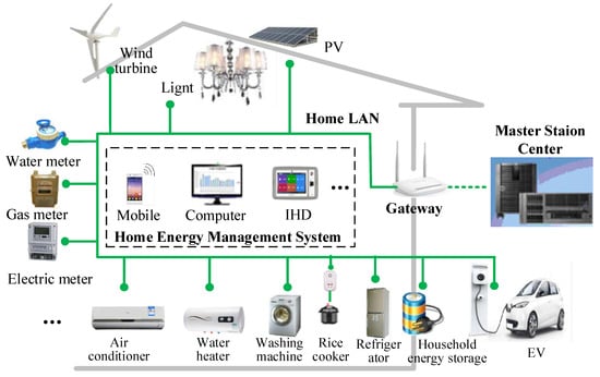
Figure 1.
A typical smart home with distributed power supply and new communicable devices.
Many studies have been carried out on home energy management, mainly involving two aspects. One is to reduce the total household energy consumption, and the other is to divert energy consumption. The former uses new energy and energy storage equipment to enhance the autonomy of power equipment. The latter reduces the power load pressure during the peak period of power consumption by shifting the working time of power-consuming equipment with high energy consumption to the reduction peak of power consumption. In terms of household energy conservation and consumption reduction, Roiné et al. [11] manage and regulate summer energy through intelligent control. The method adopts fuzzy logic rules to optimize the load consumption and ensure the reliability of the power grid by taking electricity price, renewable energy production, and load demand as variables. Mohsenian et al. [12] considered distributed energy and studied the design of an electronic device that can monitor household appliances and monitor the output of distributed power generation systems. The household load is divided into two categories, one for dishwashers which do not require human intervention, and the other for programmable household appliances such as dryers and interruptible devices such as lighting which require human intervention. Althaher et al. [13] constructed a family energy optimization control model considering real-time electricity price. The article classifies household load into two types: interruptible and non-interruptible. Different appliances adopt corresponding scheduling strategies and save electricity costs. Sabiren et al. [14] considered the influence of distributed PV by using the prediction model established by a neural network. The pre-input of neural network includes the temperature and the radiation intensity. Ciabattoni et al. [15] chose a neural network self-learning method to predict the output of a photovoltaic power generation system. The mathematical method relied on in this method is radial basis function, and the minimum resource network configuration technique and growth criterion considering pruning strategy is considered [16]. Sun et al. [17] established a control mode based on the working state of home appliances. It can be realized by switching the real-time working conditions of home appliances. After the TV is in standby, it can further choose to continue to turn off the speakers, set-top boxes, game consoles, and theater systems. Reducing energy consumption, this mode has a significant effect on saving energy. Hakan Merdanoğlu et al. [18] proposed a stochastic optimization method for the uncertainty of supply and demand and electricity price. The operation cycle of household appliances, the charging cycle of battery storage and plug-in electric vehicles, and the schedule of power purchase and sales cycle in the following days are determined. Samad et al. [19] proposed a home energy management system based on task classification, which considers the effects of economic laws and human perception on tasks in the utility function, the less sensitive the resident is to changing his/her desire task parameters, the more profit he/she will get. Alireza et al. [20] proposed a hybrid robust stochastic optimization model for smart home energy management, which considers the uncertainty of energy price and photovoltaic power generation. The total profit of day ahead and real time market can reach about $2.50 USD/day. Tasi et al. [21] focused on the energy consumed by appliances that were not fully shut down. The monitoring of these instantaneous energy values required a sensing device that could help capture and adjust the power-up state in time. The household load further reduces the unloading of the household load.
Considering the electricity price and incentive to optimize the equipment usage time, the demand response model based on the home LAN is proposed in [22], and the related equipment is used to realize the application of demand response in household energy management. The main point of [23] is to propose a pricing method for the optimal energy consumption mechanism of smart grids in the future. A demand response model based on the supply and demand sides of Steinberg’s game theory was proposed in [24]. Yong et al. [25] will satisfy the user’s maximum comfort and minimum energy cost as the objective function, and propose a new residential load management model, using the Traversal-and-Pruning algorithm to help users to rationalize equipment usage and reduce electricity consumption. Yang et al. [26] proposed a residential demand response model that uses an automatic demand response algorithm to target the minimum electricity costs of multiple homes and companies. Tsui et al. [27] developed an effective family energy management system based on demand-side management.
As the intermittent characteristic of renewable energy such as wind and solar energy, and the emergency demand response in the power system market atmosphere, the energy management of households with uncertainties has attracted huge attention. The existing research studied the optimization of the operation plan of household electrical equipment containing uncertainty from different aspects. Zhang et al. [28] established a demand response model considering user self-determination and a household electricity model with optical storage equipment. Then, a multi-time-scale family energy management model based on model predictive control was established, and the user net expenditure was proposed. The daily household electricity optimization strategy with minimum load fluctuation is the target, and the real-time power consumption adjustment strategy. By changing the battery charging and discharging, the fluctuation of the un-shifted load and the photovoltaic output during the real-time operation can be ensured to ensure that the user meets the demand response requirements. A family distributed energy random planning method based on optimal scene tree is provided in [29], which can generate a robust home electrical equipment operation plan. Kim et al. [30] considered the statistical information of users’ electricity consumption behavior and proposed a method for determining the uninterruptible load and interruptible load decision threshold of residents under real-time electricity price, which can help users save a lot of electricity consumption. In [31], based on historical load demand information, the future load is statistically estimated, and a real-time optimal management algorithm for a residential load is proposed to minimize the user’s electricity consumption. Chen et al. [32] defined an “energy adjustment variable” to model the stochastic energy consumption characteristics of various household appliances and proposed an algorithm to limit the trip rate within a certain range. Zhe He et al. [33] proposed a reliability evaluation model for internal combustion engine with comprehensive consideration of electricity, gas and heat considering the dynamic process of heat load, and conducted a case study on an internal combustion engine with four energy hubs. Kong et al. [34] introduced model predictive control technology in the family energy management system, which combines the predictive decision of the model with real-time adjustment to effectively reduce the impact of electricity price forecasting and environmental parameter uncertainty.
The uncertain parameters brought by dynamic electricity price, predicted environmental variables, and random user behavior make the original household load scheduling decision result in inevitable errors. Although the existing family energy management and optimization methods can deal with the uncertainty in the optimization of home electrical equipment operation plan to a certain extent, the following problems generally exist: (1) The number of random variables in household energy management is large, and between each other. Often not independent, there are complex coupling relationships. (2) There are not enough historical data and statistical information in reality, so it is difficult to accurately model various uncertainties with random variables. (3) The stochastic optimization problem is usually solved by the multi-scene method based on Monte Carlo sampling. The calculation amount and calculation time increase exponentially with the number of scenes and the number of random variables, which is a relatively weak and costly consideration of household energy management. A method of chance constraint programming (CCP) is proposed by Charnes and Cooper [35], mainly for the inclusion of random variables in constraints, considering the uncertain factors, allowing the decisions made to meet the constraints to a certain extent. Some achievements have been made in the optimization decision of the power system. Aiming at the maximum economic benefit of wind-storage combined unit and the minimum cost of the combined thermal-wind-storage system, an economic optimization scheduling model and solution method based on credibility theory opportunity constrained programming is constructed in [36]. The electric water heater is taken as the research object, and the opportunity constrained programming optimization scheduling model with multiple random variables is constructed, and combined with stochastic simulation and particle swarm optimization in [37,38].
For the daily optimal dispatching and emergency demand response in uncertain conditions, this paper proposes a method based on chance-constrained programming for household energy management with distributed energy source. By setting different confidence levels to reflect random variables’ influence and solved by particle swarm optimization algorithm, the scheduling strategy is obtained in different user modes. The main contributions of this paper are as follows:
- With the probability distribution of multiple random variables in power supply and load optimization scheduling, power-reduceable load, time-shifted load, and time node constrained load are constructed in this paper. Based on the dynamic priority demand response control strategy, the household load is controlled while ensuring the user’s power consumption satisfaction, thereby achieving the purpose of reducing the load.
- Considering the minimum cost of purchase and the minimum impact of comfort, the model of distributed energy source household energy management scheduling based on chance-constrained programming is established, including the daily household electricity optimization strategy and emergency demand response. The electrical adjustment strategy, combined with different tolerance schemes, verified that the decision results under the disturbance of random variables can still effectively implement power management and meet user comfort requirements.
- A solution method based on particle swarm optimization is proposed, and a flow chart is given. The solution scheme has good robustness, which proves the feasibility and effectiveness of chance-constrained programming.
The rest of the paper is structured as follows: Section 2 presents the implementation framework and main equipment model of household energy management with distributed power supply. The home energy management method for DR based on chance-constrained programming is proposed in Section 3, which includes the household energy management objective function and constraints with distributed power supply, the control strategy to participate in emergency response, and the solution method and flow chart. In Section 4, a verification example is given to verify the effectiveness of the method for home energy management simulation and home energy management simulation analysis considering emergency response is provided. Conclusions are made in Section 5.
2. Home Energy Management Architecture and Models
2.1. Implementation Architecture Design of Home Energy Management
Building a home energy management method based on opportunistic constraint planning with distributed power requires a particular implementation platform. This paper adopts a layered home energy management implementation architecture. The overall scheme is shown in Figure 2. Firstly, a prediction is based on historical data. And the next day’s load plan is obtained through the optimization algorithm. Finally, real-time controlling and emergency response adjust the plan.
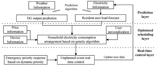
Figure 2.
Home energy management implementation architecture with distributed power.
The implementation architecture is divided into three levels, the prediction layer, the optimized scheduling layer, and the real-time control layer.
- (a)
- Prediction layer. The function of the prediction layer is mainly divided into two parts. One is to predict the distributed power output according to the weather data; the other is to record and learn the user’s usage habits through the historical data of the user’s household electricity and the next day’s users. The baseload in the family is predicted.
- (b)
- Optimized scheduling layer. The optimized scheduling layer is mainly an intelligent decision given by the smart algorithm. Based on the given next day’s electricity price information, home private equipment information, and user-set parameters, the home energy management optimization scheduling algorithm is used for daily optimization calculation, taking into account the user’s electricity comfort and benefits, and forming the next day’s electricity plan. Since the processing of distributed power sources and the behaviour of users who are consumers of electricity are inherently uncertain, uncertainty needs to be considered.
- (c)
- Real-time control layer. The real-time control layer is an implementation of the above control strategy. For the grid company’s emergency demand response, as well as the user’s accidental power usage incident, an immediate re-optimization strategy is used to re-plan the rest of the day. At the same time, to avoid the accidental event from causing excessive load on the optimization program, a user behavior learning mechanism is introduced to improve the accuracy of the primary load prediction by learning the user’s electricity usage behavior.
A schematic diagram of household energy management time, including day-ahead and emergency demand response, is shown in Figure 3. The HEMS with a distributed power supply is carried out in stages at two-time scales of emergency response and emergency demand response while meeting the multiple objectives of minimum comfort impact and minimum purchase cost. Among them, the power consumption optimization includes the power consumption plan for each period. The input quantity includes load forecasting, PV forecasting, user electricity arrangement and electricity price, and the output is the equipment running time or power; the emergency demand response is mainly used in the daytime power optimization value. Based on the incentives of the grid company, the power load adjustment and the energy storage and discharge power adjustment are carried out.
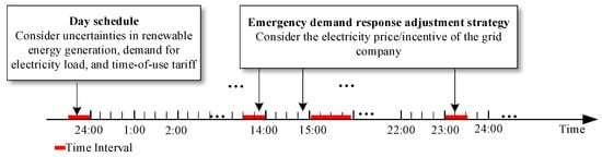
Figure 3.
Schematic diagram of household energy management time with demand response.
2.2. Household Electricity Load Model
As the user’s electricity behavior and electricity habits and the working principle of various devices are different, there are different control methods and constraints in the operation process [31]. In this paper, the load characteristics of smart home appliances are summarized as follows: power-reduceable load, time-shifted load, and time node constrained load.
2.2.1. Power-Reduceable Load
Typical interruptible load characteristics include mode switching characteristic load and indicator continuous characteristic load.
One of the advantages of smart appliances is that there are multiple intelligent modes for users to choose and intelligent switching of power gears brought by different modes. If the washing machine washes different materials and weights, choose different modes; when the water heater is heated, there are various power modes to choose from, the air purifier also has different operating modes for different air quality. If the device includes k operating modes, define its corresponding energy consumption as , in which indicates the energy consumption of the device operating in mode .
Equipment with load continuity refers to other indicators that measure the working effect in addition to working hours, such as the temperature in the air conditioning control room, and room temperature is an indicator to measure the working effect of the air conditioner. The air purifier purifies the indoor air, and the indoor air quality is an indicator to measure the working effect of the air purifier. The characteristic of this type of load is that the various indicators are continuously changed. The working effect of the previous period will have an impact on the work of the next period. The following is an example of air conditioning. The dynamic state of the air conditioning working condition and the influence on the room temperature is shown in Figure 4.
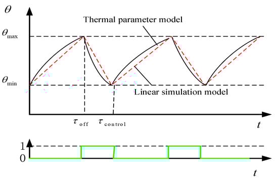
Figure 4.
Schematic diagram of air conditioner working condition and room temperature.
The schedulable capacity of the air conditioner is related to the user’s comfort requirements. The user’s temperature comfort zone can be established as a temperature zone with a temperature band between the upper and lower temperature limits. During a control cycle, when the temperature reaches the upper and lower limits, the air conditioner can be turned on or off, so that the room temperature fluctuates within a certain range. When the user’s requirements for comfort are lower, the longer the air conditioner refrigerator is allowed to turn off in one cycle, the aggregator can provide a higher compensation price to the user. Assume that the user’s requirement for indoor temperature is within the interval and that the outdoor temperature is kept constant during the direct load control period of the air conditioning load. Based on the equivalent thermal model of the air conditioning unit, the control cycle of the air conditioning load can be obtained.
where C is the equivalent heat capacity; and are the allowable indoor minimum and maximum temperature respectively; is the outdoor temperature; Rr is the room equivalent thermal resistance; η is the efficiency between cooling and power consumption; ε is the air conditioning refrigeration conversion coefficient; is the power consumption during the period; expressed as the duration of the air conditioning load regulation period; expressed as the total rated power of the user’s air conditioning load; and and are the opening and closing durations of the air conditioning load of the user respectively during the control period.
2.2.2. Time-Shiftable Load
The home energy management program issues orders that are advanced or delayed based on the original work plan for certain powered devices. For example, if the washing machine was originally planned to work after the user’s dinner, but the electricity price is higher during this period, it can be advanced to the afternoon of the afternoon electricity price to complete the laundry work, and the purpose of reducing the user’s electricity consumption is achieved. For a transferable smart appliance, the user sets the ideal work start time , maximum transfer time , and there is
Relative to time-shiftable devices, some devices, especially those that meet the basic needs of users or involve user entertainment (lights, televisions, computers, etc.), users’ satisfaction will be damaged once they have advanced or delayed. For this un-shiftable equipment, we set , therefor .
2.2.3. Time Node Constraint Load
For some device users who want to complete their work within a certain time, the user will pre-set these time parameters in the DR control terminal. For those devices whose work time is constrained. which is
where is the minimum power consumption required and and are the time when the earliest work can be started and the time when the task is completed at the latest.
Taking the electric water heater as an example, the water temperature and the amount of hot water at the time of the user’s water use affect comfort. The working model of the traditional electric water heater is that when the water temperature in the water tank of the water heater is less than or equal to the lower limit of the set temperature, the electric water heater is in a heating state, and the temperature of the hot water rises. When the water temperature in the water tank of the water heater is greater than or equal to the upper limit of the set temperature, the electric water heater is in a closed state. At this time, the hot water temperature drops due to heat loss caused by heat exchange with the environmental medium. Another important reason for the drop in warm water temperature is the constant cold-water replenishment of the electric water heater during the use of hot water. Figure 5 shows the thermodynamic temperature profile of an electric water heater without user water. The thermodynamic dynamic process of an electric water heater can be described by the following.
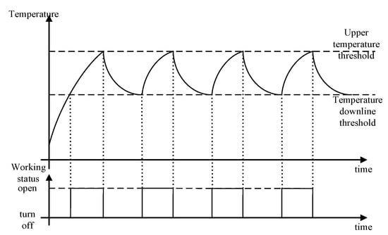
Figure 5.
Thermodynamic temperature characteristic curve of an electric water heater.
If the electric water heater is in a heating state during the period , the hot water temperature is [10]
Conversely, if the electric water heater is off during the period , there are
If there is hot water consumption during the period , the water tank of the electric water heater in the period will be supplemented with the corresponding amount of cold water, and the hot water temperature should be corrected accordingly.
where is the indoor ambient temperature; the calculated time step ; is the user’s hot water usage during the period ; is the total capacity of the electric water heater tank; is the warm water temperature before the water heater is used; is the equivalent thermodynamic parameters of the water heater underrated power heating; and R and C, respectively, indicate the thermal resistance of the electric water heater
A device with time constraints is constrained with two parameters: and . For example, in an electric car, the charging process should be completed before the user goes home from work to work the next day smoothly, so for electric cars = 18 (18:00, = 1 h), = 8 (the next day 8:00, = 1 h); and for the water heater, the user needs to use hot water before going to bed at night, the temperature of the hot water in the water heater can be as long as the user reaches the required temperature before taking a bath, as to when the water heater starts to heat up. Then, the DR program automatically optimizes according to the whole day’s electricity price, distributed power supply and household internal load conditions, and the user does not set it artificially. Therefore, the load time only has the end time parameter.
3. Home Energy Management Method for DR Based on Chance-Constrained Programming
3.1. Objective Function and Constraints with Distributed Power Supply
Relying on the intelligent dispatch management of the family, users can not only reduce the waste of home appliances through optimization control but also save money on electricity purchases. They can also use some methods to save electricity. For example, (1) reasonably transfer the running time of household appliances, minimize the period of use of electricity, that is, the period of high electricity price; (2) combine the power generation of local renewable energy with energy storage equipment and use the power generated by distributed power generation system or energy storage equipment during the peak period of power consumption. The excess energy released in the middle reduces the cost of purchasing electricity from the home user to the power company. In addition, the distributed generation system and the energy storage system can also sell excess electric energy to the power company for profit. The energy storage device can store electric energy during the low peak period of electricity consumption and release the electric energy to the home appliance during the peak period of power consumption.
Figure 6 shows the structure of the scheduling algorithm for minimizing the user’s electricity purchase cost. The scheduling object includes the local renewable energy power generation system, household appliances, and energy storage reserves. The control strategy aims to make full use of renewable energy, comfort, and minimize the cost of electricity purchase. The degree of influence is minimal, and the constraints include the working characteristics of the household electrical appliance, the preference of the user, and the charging and discharging power of the energy storage device.
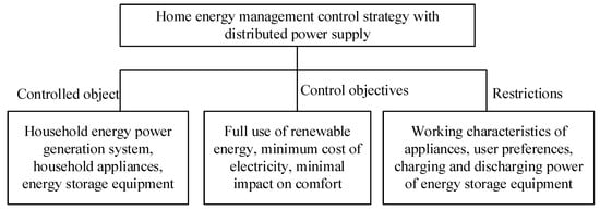
Figure 6.
Distributed power supply family energy management algorithm structure diagram.
3.1.1. Objective Function
The paper considers both price-based demand response and incentive-type demand response. Among them, the day-to-day scheduling is in the form of considering the price-type demand response and adopts the form of time-sharing electricity price. The daily emergency demand response adopts the incentive-type compensation mechanism and uses the power compensation of peak clipping or power failure (¥/kW∙h). The optimization of home energy management is to achieve economic and comfort coordination through the energy planning of the user’s internal equipment. The objective function of the home daily load planning is as follows:
where and are the cost of the user’s economical cost and satisfaction, respectively; and are the constant-coefficient and the weight coefficient between the economic cost and the comfort cost, which + = 1. They represent a variety of modes, from the “saving mode” that saves electricity bills to the “equalization mode” that takes into account economy and comfort and the “comfort mode” that focuses on comfort while increasing. The user can set the mode of the next optimization cycle before the start of each optimization cycle to realize a more flexible and interactive intelligent power consumption mode.
Since the distributed power supply is installed in the user’s home, when calculating the economy, it is necessary to remove this part of the load. The electricity price model considered in this paper is the time-of-use electricity price, and the economic cost is expressed as follows:
where is the purchase of electricity for the family at t period. When the renewable energy generation is greater than the required power (); is the power consumed by device i and is the device state at t period, and when the device is off; is the cost of electricity purchase for household electricity at time t; is the time-of-use electricity price that represents t-time, usually including peak, low-valley, and various types; is the average compensation price for incentives for grid companies to implement emergency demand response at time t. In the absence of date demand-side management period, .
The user’s satisfaction cost expression is set as
where , , , and are the different weighting coefficients that characterize the changes in equipment operating time, changes in operating mode, and completion of indicators on user comfort, which can be set by user with the habit and preference.
Since the changing of power consumption time, the above various load control methods will cause the deviation between the device working state and the ideal situation to more or less impair the user’s satisfaction. Therefore, the degree of deviation between the actual working state of the device and the ideal working state is used as a measure of the damage to the user satisfaction of the demand response program. This part is actually a kind of cost for users to use electricity, called the cost of satisfaction. For devices with transferable load characteristics. If the ideal usage time of the device is , the expression of the satisfaction cost is as follows.
where and are constant-coefficient to measure the degree of damage to the user’s satisfaction caused by the delay or early use of the device.
For the device with mode switching characteristics, if the ideal working mode of the device is , the expression of the satisfaction cost is as follows.
where and are constant coefficient, which is used to measure the degree of damage to the user’s satisfaction by changing the operating mode of the device in order to save electricity costs.
For the continuous indicator appliances, we use the deviation between the current indicator and the corresponding indicator to measure the upper and lower limits of the corresponding indicator, the upper limit is , and the lower limit is . In the case of emergency response, the percentage of indicator deviation is used as the corresponding satisfaction cost. In the energy optimization calculation, if it is not crossed, it is considered that user satisfaction is not impaired, and the same calculation method as the emergency response is adopted. If the ideal index value of the device is , the corresponding index value of the current task is , in the energy optimization problem, the satisfaction cost expression is
For the time-constrained load characteristics, on the one hand, it is considered that as long as the task is completed within the user-defined interval, the user satisfaction is not damaged, or the damage caused can be neglected; that is, the required task is completed on time, and the satisfaction cost is zero. On the other hand, if the work is not completed on time, for example, the electric car does not complete charging before the user goes out to work the next morning, the damage to the user’s satisfaction is huge, and at this time, it is considered as a non-opportunity constraint, and the type of satisfaction cost is infinite.
3.1.2. Constraints
The family energy management constraints mainly involve the working characteristics of household electrical appliances, the preferences of users, and the charging and discharging power of energy storage equipment.
- Uncontrollable appliance
The power of such equipment shall not exceed the maximum-minimum power limit during the initial running time and the end running time, so the constraint on electric energy consumption is expressed as
- Time-shifted appliance
The power of such appliance shall not exceed the maximum and minimum power limits during the initial running time and the end running time. In addition, during this period of time, the power consumption of the equipment must exceed the minimum threshold, and the work is considered completed. Unify the model of household controllable electrical equipment. Therefore, the constraint on the amount of energy consumed is expressed as
- Energy storage equipment charging and discharging
Since the state of the energy storage equipment is continuously changing, the model of the energy storage equipment must be transformed into a decisional and operational method before the microgrid optimization scheduling is solved [27]. The state of charge (SOC) allowed by the energy storage device is discretized, and the work area is divided into N shares, forming a state set , which is expressed as
where the state of charge of the energy storage element at the end of the t stages is represented by st and is used as the decision variable of the energy management optimization control and has , (%). The maximum and minimum state of charge allowed for the energy storage device, respectively and . Due to the limitation of the charging and discharging current of the energy storage device, the energy storage state changes in adjacent stages are limited, and the charging and discharging of the energy storage equipment in each stage should satisfy
where and represent the maximum charge and discharge rate of the energy storage device, and the value is determined by the charge and discharge characteristics of the energy storage device.
If the charge and the discharge amount of the energy storage in the t period is described by xt, the value is related to the initial stage state st-1 and the stage decision variable sk. The amount of charge and discharge power required by the energy storage device is determined by its own charge and discharge characteristics and the state of the previous stage. From the state st-1 to st, according to [21]
where is the capacity of the energy storage device; is the self-discharge rate of the energy storage device; and and are the charging and discharging efficiency of the energy storage medium.
3.2. Energy Management Strategy Based on Chance-Constrained Programming
3.2.1. Model Construction Based on Chance-Constrained Programming
The existence of multiple random variables leads to the original mathematical programming problem becoming an uncertain programming problem. Chance constraint planning involves random variables in the constraints, considering the uncertain factors, allowing the decisions made to meet the constraints to a certain extent.
Set as the decision vector of HESM and is the unpredictable random variable at t period. To minimize the objective function of (11), the chance-constrained programming model with random variables is given as follows [17]
where is the probability that the event , is the confidence level of the constraint given in advance. In the chance constraint, the decision vector is a feasible solution if only , and the probability value of the event is not smaller than . For inelastic constraints, take .
In this paper, the first type of constraint (uncontrollable load) is set, and the third type of constraint (charge and discharge constraint of energy storage) is an inelastic constraint; the second type of constraint (time-shifted device) is the elastic constraint. The random variables in the optimal scheduling model for air conditioners, electric water heaters, etc., are the ambient temperature predicted before, the amount of user hot water, etc., and only appear in the constraint conditions. Uncertain constraints in the objective function include the amount of electricity generated by renewable energy and the cost of purchasing electricity. The main decision variables and random variables of the household energy management system covered in this paper are shown in Table 1.

Table 1.
Main decision and random variables of the energy management system covered in this paper.
The chance-constrained programming is used to deal with the home energy management optimization scheduling model with random variables. The form is as follows:
According to the CCP theory, the confidence level is used to limit the degree of violation of the opportunity constraint. From the user’s point of view, reflects the user’s tolerance for abuse of the power habits, which reflects the user’s consideration of the comfort of a device. If , it means that the user has strict requirements on the use of the device, and no matter how the random variable changes, it cannot violate its constraints. Otherwise indicates that the user is completely unconcerned about the scope of the power usage habit, which is approximately equal to the unconstrained condition.
Considering that there are a large number of constraints in the optimal scheduling model, to unify the objective function and constraints, this paper adds a penalty function to the objective function to deal with the constraints. The penalty function designed in this paper is as follows:
when designing the penalty function, we consider that the penalty function value is 1 when the constraint is violated under different confidence levels. Such a design strictly guarantees that the degree of punishment for each constraint is consistent in the objective function. Through the design of the above penalty function, the entire constrained family energy management problem is transformed into an unconstrained optimization problem.
where is the penalty coefficient. From the mathematical point of view, the problem of optimal scheduling of electric water heaters is finally transformed into an unconstrained nonlinear integer programming problem that is easy to solve.
In the solution of HEMS, the decision at each moment in the entire time period are considered. As shown in Equations (28) and (31), the main idea of the proposed method in this paper is to minimize the cost of electricity purchase and comfort by dynamically and continuously making decision variables for each period. Based on determined in the previous period, making a short-term forecast of the load; and considering the power output of DG and other key parameters given at this stage, such as provided by the grid company and set by the user, the decision solution is obtained, which has the goal to minimize f(∙) in the entire period of . The model is a multi-stage decision-making problem, which can be solved using dynamic programming methods. Figure 1 shows the process of solving the above model, and more details are present in [34].
Based on the HEMS status at the end of the energy management period, the optimal scheduling solution can be acquired from [xt−1, xt] in each time interval and then the corresponding values are also obtained. The reverse search process for the optimal scheduling is shown in Figure 7 and Figure 8. The proposed method model separates the factors of market environment and the method of modelling the operating cost function at each stage (i.e., each time step). Compared to existing works, the proposed method is able to help the system operators realize an optimal energy management by (1) creatively adapting various market structures with strong robustness; (2) relevant factors such as supplementary price of DR, power consumption constraint of users, and the characters of different types of equipment can be considered; and (3) efficiently solving the HEMS energy management problem, which can be further summarized to develop expert knowledge for real-time operation.
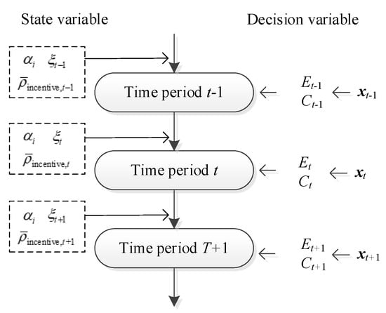
Figure 7.
Multi-stage process for solving the proposed model.
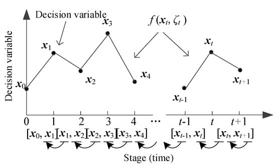
Figure 8.
Reverse search process for optimal scheduling based on dynamic consecutive decision making.
3.2.2. Control Strategy Adjustment for Participation in Emergency Response
If there is no battery or the battery is inefficient, the electric power or the translation load of the equipment can be adjusted to respond to the renewable energy generation. As a temporary event, the emergency demand response project has a large adverse impact on the user’s life without prior planning. Therefore, one of the main purposes of the control strategy design is to minimize the impact and damage to the user. The control flow of HEMS based on chance-constrained programming as shown in Figure 9.
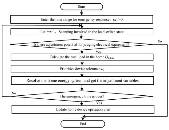
Figure 9.
Control flow of home energy management system (HEMS) based on chance-constrained programming.
The specific control steps are as follows:
- Accept the demand response command and enter the time range for the emergency demand response.
- Scan the home internal load QL,total, and determine whether the total load inside the home exceeds the EDR power limit QRE,limit. If yes, start the program.
- Judging the working state of the three types of electrical equipment. If all three loads are in the off state, the procedure ends directly (ie, the household cannot contribute to the grid’s load reduction); otherwise, it proceeds to step 6).
- Based on the user’s electricity habits and consideration of comfort, prioritize the power equipment to improve the equipment tolerance ai with low priority.
- Re-solve the home energy system and obtain adjustment variables. Determine whether the emergency response period of the home is over; if not, repeat steps 2) to 4); if yes, proceed to the next round of control.
- Update the home equipment operation plan.
- Save the emergency demand response to the energy management results of the home device and end.
3.3. Solution for the Proposed Home Energy Management at t Period
The position and velocity of the particle in the space are respectively and , and the optimal position of the particle is , the optimal position of all particles is, then each particle updates its speed and position by the following formula:
where is the inertia weight; and are the positive learning factor; and the random number between 0 and 1. Since the above-optimized scheduling model is a 0–1 programming problem, the binary coded discrete particle swarm optimization algorithm is more suitable for solving [22].
The particle velocity will be limited to the range , and its position update formula is
The specific process is as follows:
- Read in the data. Read the range of parameters such as renewable energy generation (QPV,t, QWT,t), indoor and outdoor ambient temperature (), and user hot water consumption () predicted in an uncertain environment; read the energy management model parameters and particle swarm algorithm parameters; users also need to set the parameter constraint limit range and constraint confidence level according to their own power characteristics and habits.
- Calculate the probability distribution function of parameters such as renewable energy generation, indoor and outdoor environmental temperature, and user hot water usage based on historical information and read data, and form a set of initial variables , as the initial set of particle swarm optimization algorithm. Population randomly initializes the position and velocity of each particle in the particle population.
- Using the stochastic simulation method to deal with the opportunity constraints: set , according to the random variable probability distribution function to generate an independent random variable as a sample, and select any given decision variable x to bring the sample into the constraint, if the constraint is met , then . Repeat this way, according to the significant number theorem, when is large enough, the value is regarded as the actual probability of the opportunity constraint. If , the example generated by the particle swarm algorithm does not meet the probability level, and the particle needs to be discarded, and return to Step 2).
- When all the particles satisfy the condition, the N objective function values generated by the scheduling scheme obtained by each operation are sorted. The ranking of is started, the sequence is obtained, and the penalty function value of the constraint condition is calculated. The sum of the objective function value and the penalty function value is taken as the fitness of each particle, and the individual corresponding to the fitness of all individuals is the optimal value of the objective function.
- The target value obtained in Step 4 is directly used as the fitness, and the fitness of each particle is compared with the fitness corresponding to the best position it has experienced. If it is better, it is the current best position. Compare the current fitness value and corresponding fitness value of all particles, update the value .
- Update the particle velocity and position, and iteratively calculate the population to obtain a new generation.
- Repeat Steps 3) to 6) to search for the optimal solution by changing the value of the confidence level. If the stop condition is satisfied (usually the preset operation precision or the number of iterations), the search stops and the best particle is given as the optimal solution.
The solution process of the family energy management algorithm based on particle swarm is shown in Figure 10.
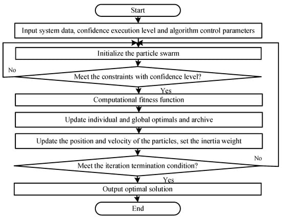
Figure 10.
Family energy management solution process based on the particle swarm optimization algorithm.
4. Case Study
4.1. Basic Condition
The time-of-use (TOU) price is a common demand-side management method, which have different electricity prices at period of peak, flat, and valley time. Users consciously adjust their power equipment to achieve “peak shaving and valley filling” of the power grid, which is beneficial to alleviate the pressure on the power grid and promote the safe operation of the power grid. The simulation of this example uses the TOU price and the electricity price of each period when the family purchases electricity from the grid company is shown in Table 2.
Table 2.
Time-of-use tariffs for households purchasing electricity from grid companies.
Uncontrollable equipment (also known as baseload) within a resident’s home cannot be controlled through a home energy management program. The previous models and algorithms in this paper were all directed at controllable loads. The PV on-grid price is also based on the peak and valley electricity price. The peak electricity price is 0.73 ¥/kW∙h, and the valley time is 0.13 ¥/kW∙h, other time usually is 0.38 ¥/kW∙h. The PV output forecast and the baseload are shown in Figure 11. The internal load of the home is shown in Table 3.
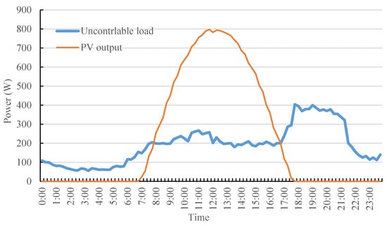
Figure 11.
Schematic diagram of baseload and PV output prediction.
Table 3.
Household appliances.
The outdoor ambient temperature is 30 °C; the initial room temperature is 27 °C, the initial water temperature is 55 °C; the initial SOC of the electric vehicle is 30%, charging to 100% is the completion of the work; the electric vehicle can complete the charging task in 6 h under the rated power. It takes 3 min for each hot water in the water heater to rise once, and 4 h for the hot water to cool naturally at 10 degrees Celsius; after the air conditioner reaches the set temperature, the working frequency is 15 min, and the air conditioner works in a cooling state.
The distributed power supply of PV adopts the mode of “spontaneous self-use, surplus surfing the Internet,” in which the electricity generated by distributed power supply is first used by HESM for spontaneous self-use and then sold to the power grid when the remaining electricity is available. This model is one of the most important forms of distributed power supply operation in China. The working conditions of the equipment inside the home do not consider the demand response of TOU and the total load curve of the family in one day are shown in Figure 12.
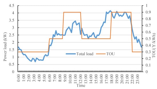
Figure 12.
Total load curve in the household before participating in normal day.
4.2. Home Energy Management Simulation under Normal Conditions
Set the particle swarm size to 50, that is, 50 individuals per generation; the maximum number of iterations is 300 generations. In this paper, the load power distribution in the home is optimized and simulated, and the total load curve is shown in Figure 13. It can be seen from the figure that the working time of the equipment has shifted, and the maximum peak of the household load has been shifted from the peak period before the optimization to the flat period. According to the calculation, the electricity RMB bill is reduced from the previous ¥39.26 to ¥37.71, saving about 3.948% of the electricity cost. It shows that the optimization algorithm saves the user the cost of electricity consumption is very significant. Figure 14 and Figure 15 show the operational status of water heater and EV loads in the DR case of TOU price.
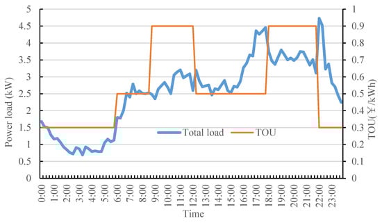
Figure 13.
Total load curve with the demand response (DR) of time-of-use (TOU) price.
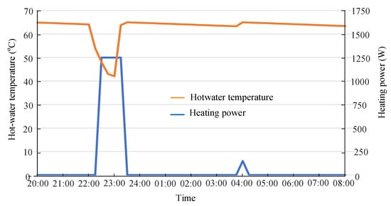
Figure 14.
Working status of the water heater under normal conditions.
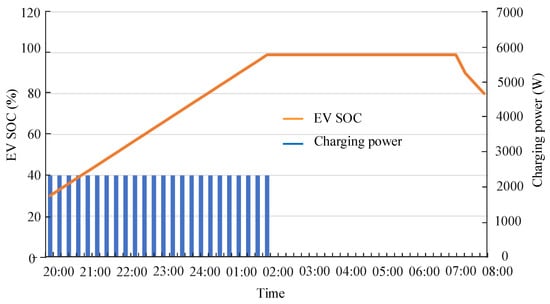
Figure 15.
Charging status of EV under normal conditions.
The above discussion is based on the zero tolerance () case, which is an extreme case. Since the ambient temperature and water consumption are uniformly distributed random variables, the user can give a certain degree of tolerance to the temperature constraints to achieve the purpose of reducing electricity charges. At this point, the user can achieve a balance between comfort and electricity by setting the confidence level. At this time, the electricity fee values calculated under different confidence levels are shown in Table 4.
Table 4.
Electricity price at different confidence levels.
From the table, it can be found that the zero-tolerance scheme is the one with the highest cost of electricity. This is because the zero-tolerance scheme has the most stringent constraint requirements, which inevitably leads to an increase in the user’s electricity bill. As the level of confidence decreases, the user’s tolerance for constraints becomes greater, and the user’s electricity bill will continue to decrease. This economic gain is due to the user’s sacrifice of comfort. Users can set different usage modes according to tolerance. For example, low tolerance is a comfortable mode, and high tolerance is the economic mode. The actual water temperature curves at 0.8, 0.6, 0.4, and 0.2, respectively, are shown in Figure 16. It can be seen that the real water temperature curve’s violation of the constraint increases as the confidence level decreases.
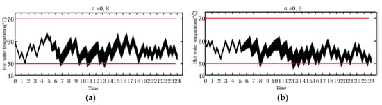
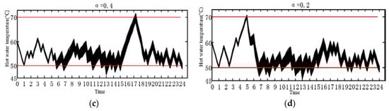
Figure 16.
Actual water temperature curve at different confidence levels.
Due to different usage habits of the user, the comfort interval set by the user may vary. For example, the user may have a proper partial heat when the bath is required, and the water temperature is suitably cold during the rest of the period. In order to discuss the time-varying temperature constraint interval, the user is set to a low water temperature period from 18:00 to 22:00, at which time the water temperature setting is reduced by 5 °C compared to the constant temperature constraint interval. Table 2 shows the changes in the user’s electricity bill when the confidence level is continuously lowered. Figure 16 shows the actual water temperature curve for the zero-tolerance scheme under the time-varying temperature constraint interval.
To verify the influence of the fluctuation of the output of renewable energy, the deviation of PV is set to be 20% of the predicted value. The PV prediction and actual output curve are shown in Figure 17. The shaded part is the uncertainty set constructed in this chapter. At the same time, GAN is used to generate 20 electric, thermal and cold scenes, and k-medoids algorithm is used to reduce them to three scenes. The scenes and actual values after the reduction are shown in Figure 18.
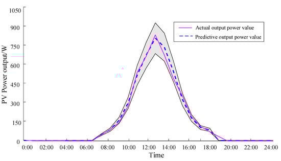
Figure 17.
PV prediction and actual output curve.
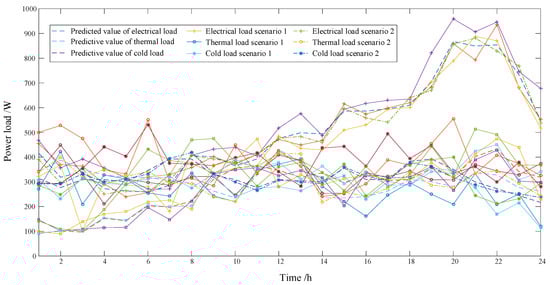
Figure 18.
Family load result curves in different scenarios based on HEMS.
The weather and the device state of distributed power supply will affect the solution result of HEMS, and different conditions are used for analysis. Data1, Data1, and Data3 are the convergence of the proposed method and the user’s electricity cost results under the weather conditions of sunny, cloudy, and rainy with distributed power supply normal operation, respectively; Data4, Data5, and Data6 are the data under the condition of 20% aging of distributed power installations for sunny, cloudy and rainy. The cost results curves of the proposed method with different cases in generations are shown in Figure 19. It can be seen from the curves that the total cost of user is lowest in sunny. Further, to analyze the effect of the proposed method with other algorithms, such as the Simulated Annealing (SA) method and Genetic Algorithm (GA) method, the comparison of the convergence and results of different solving methods with Data 6 are obtained and shown in Figure 20.
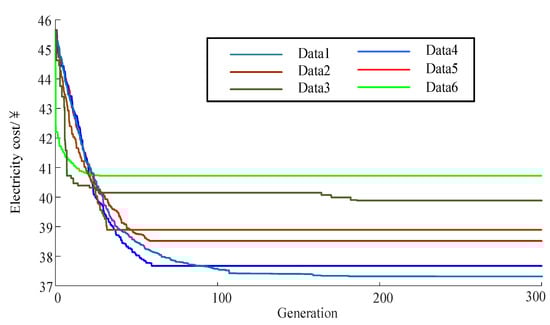
Figure 19.
Cost results curves in generations with different cases.
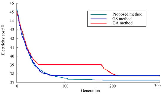
Figure 20.
Comparison of the convergence and results of different solving methods with Data 6.
4.3. Home Energy Management Simulation for Emergency Demand Response
The loads involved in emergency response are water heaters, air conditioners and electric vehicles. The equipment information of the three loads involved in the emergency demand response is shown in Table 5. Among them, the water heater and the air conditioner are set by the user to allow the water temperature and the fluctuation range of the room temperature; the electric vehicle is set by the user to complete the charging task at the latest.
Table 5.
Load equipment information participating in emergency demand response.
With the reasons of power grid failures and others, the emergency demand response from 22:30 to 23:30 are required to reduce users power consumption. Figure 21, Figure 22 and Figure 23 show the working status of various loads with the emergency demand response.
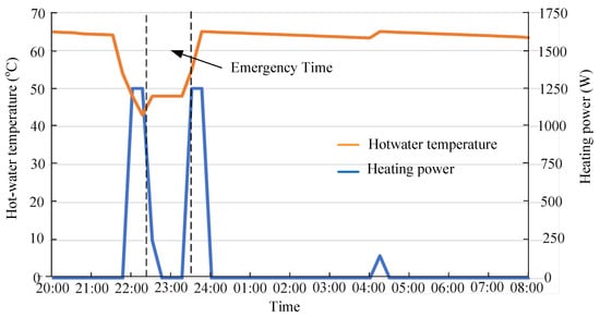
Figure 21.
Working status of the water heater in response to emergency demand response.
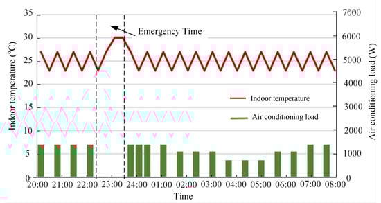
Figure 22.
Air conditioner working status in response to emergency demand response.
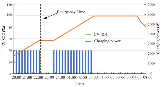
Figure 23.
Working status of EV charging in case of emergency response.
With the dynamic changes in priority of three devices, a schematic diagram of the total load change in the home before and after the emergency DR is shown in Figure 24. The final conclusion is that the method proposed in this paper can meet the demand response of power grid companies and obtain a lower energy cost.
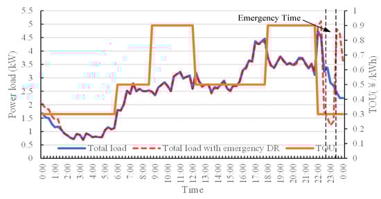
Figure 24.
Total load changes in the household during emergency response.
Since the electric vehicle is in a state in which the charging task can be completed within the response time period, the electric vehicle has the lowest priority and first responds to the control. The priority of air conditioners and water heaters alternates. It can be seen from the comparison before and after the proposed dynamic priority emergency response control strategy, which can effectively reduce the load inside the home and ensure the user’s power consumption satisfaction. For the different incentive prices () in Equation (14), Table 6 gives the variation between the degree of compensation and the amount of response. As the unit’s power consumption increases, a positive correlation between the demand response compensation price and the user’s reduction is verified.
Table 6.
Users’ compensation under different emergency response incentives.
5. Conclusions
This paper proposes the household energy optimization management for demand response with distributed power supply. Based on load characteristics combination, an opportunity constrained programming model is established, which solves the model by combining stochastic simulation and particle swarm optimization. The zero-tolerance scheme is given, and the simulation results show that the decision-making results can meet the user comfort requirements under the disturbance of random variables. The solution scheme has good robustness, and it also proves that chance-constrained programming is feasible and effective solving home energy scheduling problem under the uncertain environment. When different confidence levels are set to reflect the tolerance of users, the results prove that the user can tolerate a certain degree of comfort in exchange for the appropriate economy.
Author Contributions
Conceptualization, X.K. and Q.Y.; methodology, B.S. and Q.Y.; software, B.S. and S.Z. (Siqiong Zhang); validation, S.L.; formal analysis, S.Z. (Shijian Zhu), and B.S.; data curation, X.K., Q.Y. and B.S.; writing—original draft preparation, S.Z. (Siqiong Zhang), B.S., and Q.Y.; writing—review and editing, X.K., S.Z. (Shijian Zhu) and B.S.; supervision, Q.Y., S.L., and B.S. All authors have read and agreed to the published version of the manuscript.
Funding
This research was funded by the National Natural Science Foundation of China under grant no. 51877145.
Acknowledgments
The authors would like to acknowledge the support in part by the Electric Power Research Institute of Tianjin Power Grid.
Conflicts of Interest
The author declares no conflict of interest. The funders had no role in the design of the study; in the collection, analyses, or interpretation of data; in the writing of the manuscript; and in the decision to publish the results.
Abbreviations
| DR | Demand response |
| DG | Distributed generation |
| PV | Photovoltaic |
| HEMS | Home energy management system |
| IHD | Internet Handheld Devices |
| LAN | Local area network |
| HES | Household energy storage |
| EV | Electric vehicle |
| CCP | Chance Constraint Programming |
References
- Bhuvanesh, A.; Jaya Christa, S.T.; Kannan, S.; Karuppasamy Pandiyan, M. Multistage multiobjective electricity generation expansion planning for Tamil Nadu considering least cost and minimal GHG emission. Int. Trans. Electr. Energy 2019, 29, e2708. [Google Scholar] [CrossRef]
- Zhou, Y. Optimal Scheduling Methods for Demand Response Resources at the User Side; Tianjin University: Tianjin, China, 2016. [Google Scholar]
- Han, D.M.; Lim, J.H. Smart home energy management system using IEEE 802.15.4 and zigbee. IEEE Trans. Consum. Electron. 2010, 56, 1403–1410. [Google Scholar] [CrossRef]
- Tehrani, K.; Maurice, O. A cyber physical energy system design (CPESD) for electric vehicle applications. In Proceedings of the 2017 12th System of Systems Engineering Conference (SoSE), Waikoloa, HI, USA, 18–21 June 2017; pp. 1–6. [Google Scholar]
- Amirahmadi, A.; Rafiei, M.; Tehrani, K.; Griva, G.; Batarseh, I. Optimum Design of Integer and Fractional-Order PID Controllers for Boost Converter Using SPEA Look-up Tables. J. Power Electron. 2015, 15, 160–176. [Google Scholar] [CrossRef]
- Ali, S.M.; Ullah, Z.; Mokryani, G.; Khan, B.; Hussain, I.; Mehmood, C.A.; Farid, U. Smart grid and energy district mutual interactions with demand response programs. IET Energy Syst. Integr. 2019, 2, 1–8. [Google Scholar] [CrossRef]
- Kong, X.; Xiao, J.; Wang, C.; Cui, K.; Jin, Q.; Kong, D. Bi-level multi-time scale scheduling method based on bidding for multi-operator virtual power plant. Appl. Energy 2019, 249, 178–189. [Google Scholar] [CrossRef]
- Grogan, A. Smart appliances. Eng. Technol. 2012, 7, 44–45. [Google Scholar] [CrossRef]
- Chen, F.; Huang, G.; Fan, Y.A. linearization and parameterization approach to tri-objective linear programming problems for power generation expansion planning. Energy 2015, 87, 240–250. [Google Scholar] [CrossRef]
- Gitizadeh, M.; Kaji, M.; Aghaei, J. Risk based multiobjective generation expansion planning considering renewable energy sources. Energy 2013, 50, 74–82. [Google Scholar] [CrossRef]
- Roiné, L.; Therani, K.; Manjili, Y.S.; Jamshidi, M. Microgrid energy management system using fuzzy logic control. In Proceedings of the 2014 World Automation Congress (WAC), Waikoloa, HI, USA, 3–7 August 2014; pp. 462–467. [Google Scholar]
- Mohsenian-Rad, A.H.; Leon-Garcia, A. Optimal Residential Load Control with Price Prediction in Real-Time Electricity Pricing Environments. IEEE Trans. Smart Grid 2010, 1, 120–133. [Google Scholar] [CrossRef]
- AIthaher, S.; Mancarella, P.; Mutale, J. Automated Demand Response from Home Energy Management System Under Dynamic Pricing and Power and Comfort Constraints. IEEE Trans. Smart Grid 2015, 6, 1874–1883. [Google Scholar] [CrossRef]
- Saberian, A.; Hizam, H.; Radzi, M.A.M.; Ab Kadir, M.Z.A.; Mirzaei, M. Modelling and Prediction of Photovoltaic Power Output Using Artificial Neural Networks. Int. J. Photoenergy 2014, 2014. [Google Scholar] [CrossRef]
- Ciabattoni, L.; Grisostomi, M.; Ippoliti, G.; Longhi, S. Neural networks based home energy management system in residential PV scenario. In Proceedings of the 2013 IEEE 39th Photovoltaic Specialists Conference (PVSC), Tampa, FL, USA, 16–21 June 2013; pp. 1721–1726. [Google Scholar]
- Al-Messabi, N.; Goh, C.; El-Amin, I.; Li, Y. Heuristically enhanced dynamic neural networks for structurally improving photovoltaic power forecasting. In Proceedings of the International Joint Conference on Neural Networks, Beijing, China, 6–11 July 2014; pp. 2820–2825. [Google Scholar]
- Byun, J.; Park, S.; Kang, B.; Hong, I.; Park, S. Design and implementation of an intelligent energy saving system based on standby power reduction for a future zero-eneigy home environment. IEEE Trans. Consum. Electron. 2013, 59, 507–514. [Google Scholar] [CrossRef]
- Merdanoğlu, H.; Yakıcı, E.; Doğan, O.T.; Duran, S.; Karatas, M. Finding optimal schedules in a home energy management system. Electr. Power Syst. Res. 2020, 182, 106229. [Google Scholar] [CrossRef]
- Samadi, A.; Saidi, H.; Latify, M.A.; Mahdavi, M. Home energy management system based on task classification and the resident’s requirements. Int. J. Electr. Power Energy Syst. 2020, 118, 105815. [Google Scholar] [CrossRef]
- Akbari-Dibavar, A.; Nojavan, S.; Mohammadi-Ivatloo, B.; Zare, K. Smart home energy management using hybrid robust-stochastic optimization. Comput. Ind. Eng. 2020, 143, 106425. [Google Scholar] [CrossRef]
- Tasi, C.H.; Bai, Y.W.; Chu, C.A.; Chung, C.Y.; Lin, M.B. Design and implementation of a socket with ultra-low standby power. In Proceedings of the IEEE Instrumentation and Measurement Technology Conference, Binjiang, China, 10–12 May 2011; pp. 1–6. [Google Scholar]
- Pipattanasomporn, M.; Kuzlu, M.; Rahman, S. Demand response implementation in a home area network: A conceptual hardware architecture. In Proceedings of the IEEE PES Innovative Smart Grid Technologies (ISGT), Washington, DC, USA, 16–20 January 2012; pp. 1–8. [Google Scholar]
- Wang, X.; Kong, X.; Sun, F.; Zhang, C. Research on Multi-Energy Coordinated Intelligent Management Technology of Urban Power Grid under the Environment of Energy Internet. Appl. Sci. 2019, 9, 2608. [Google Scholar] [CrossRef]
- Samadi, P.; Schober, R.; Wong, V.W.S. Optimal energy consumption scheduling using mechanism design for the future smart grid. In Proceedings of the 2011 IEEE International Conference on Smart Grid Communications, Brussels, Belgium, 17–20 October 2011; pp. 369–374. [Google Scholar]
- Yong, C.; Kong, X.; Chen, Y.; Cui, K.; Wang, X. Multi-objective Scheduling of an Active Distribution Network Based on Coordinated Optimization of Source Network Load. Appl. Sci. 2018, 8, 1888. [Google Scholar] [CrossRef]
- Yang, J.; Zhang, G.; Ma, K. Demand response based on stackelberg game in smart grid. In Proceedings of the 32nd Chinese Control Conference, Xi’an, China, 26–28 July 2013; pp. 8820–8824. [Google Scholar]
- Tsui, K.M.; Chan, S.C. Demand response optimization for smart home scheduling under real-time pricing. IEEE Trans. Smart Grid 2012, 3, 1812–1821. [Google Scholar] [CrossRef]
- Zhang, Y.; Kong, X.; Sun, B.; Wang, J. Multi-Time Scale Home Energy Management Strategy Based on Electricity Demand Response. Power Syst. Technol. 2018, 42, 1811–1818. [Google Scholar]
- Wang, C.; Zhou, Y.; Wang, J. A novel traversal-and-pruning algorithm for household load scheduling. Appl. Energy 2013, 102, 1430–1438. [Google Scholar] [CrossRef]
- Kim, T.T.; Poor, H.V. Scheduling power consumption with price uncertainty. IEEE Trans. Smart Grid 2011, 2, 519–527. [Google Scholar] [CrossRef]
- Samadi, P.; Mohsenian-Rad, H.; Wong, V.W.; Schober, R. Tackling the load uncertainty challenges for energy consumption scheduling in smart grid. IEEE Trans. Smart Grid 2013, 4, 1007–1016. [Google Scholar] [CrossRef]
- Chen, X.; Wei, T.; Hu, S. Uncertainty-aware household appliance scheduling considering dynamic electricity pricing in smart home. IEEE Trans. Smart Grid 2013, 4, 932–941. [Google Scholar] [CrossRef]
- Hou, K.; He, Z.; Wang, Y.; Jia, H.; Zhu, L.; Lei, Y.; Liu, X.; Yu, X. Reliability modeling for integrated community energy system considering dynamic process of thermal loads. IET Energy Syst. Integr. 2019, 1, 173–183. [Google Scholar] [CrossRef]
- Kong, X.; Bai, L.; Hu, Q.; Li, F.; Wang, C. Day-ahead optimal scheduling method for grid-connected microgrid based on energy storage control strategy. Mod. Power Syst. Clean Energy 2016, 4, 648–658. [Google Scholar] [CrossRef]
- Charnes, A.; Cooper, W.W. Chance-constrainted programming. Manag. Sci. 1959, 6, 73–79. [Google Scholar] [CrossRef]
- Ma, L.; Wang, Z.; Lu, X. Optimal Scheduling of Combined Wind-thermo-storage System Based on Chance-constrained Programming. Power Syst. Technol. 2019, 43, 3311–3320. [Google Scholar]
- Zeng, B.; Jiang, W.; Yang, Z. Optimal load dispatching method based on chance-constrained programming for household electrical equipment. Electr. Power Autom. Equip. 2018, 38, 27–33. [Google Scholar]
- Li, M.; Huang, L.; Li, J. Distribution System Reliability Assessment Software Based on Bayesian Network and Sequence Simulation. Sci. Technol. Eng. 2013, 13, 70–74. [Google Scholar]
© 2020 by the authors. Licensee MDPI, Basel, Switzerland. This article is an open access article distributed under the terms and conditions of the Creative Commons Attribution (CC BY) license (http://creativecommons.org/licenses/by/4.0/).