Methodology for Tuning MTDC Supervisory and Frequency-Response Control Systems at Terminal Level under Over-Frequency Events

Abstract

This paper proposes a methodology for tuning a supervisory and frequency-response outer loop control system of a multi-terminal direct current (MTDC) grid designed to transmit offshore wind energy to an onshore AC grid, and to provide frequency support during over-frequency events. The control structure is based on a master–slave scheme and ensures the achievement of frequency response, with specific implementation of the UK national grid code limited-frequency sensitive (LFSM) and frequency-sensitive (FSM) modes. The onshore AC grid is modelled with an equivalent frequency-response model to simulate the onshore AC grid dynamics under frequency deviations. The main innovation of this paper is the development of a methodology for tuning simultaneously two hierarchical levels of a MTDC coordinated control structure, i.e., the MTDC supervisor, given by the active power set point for slave terminal, and the slope of frequency-response functions at onshore terminals. Based on these two hierarchical levels, different strategies are evaluated in terms of frequency peak reductions and change of the frequency order type. Moreover, tuning guidance is given when a different MTDC control structure or different synchronous generator characteristics of the onshore AC grid are considered.

1. Introduction

The compliance with grid codes is a mandatory aspect in renewable energy integration and each country decides upon their governing rules [1]. It is the task of the control architecture not only to guarantee the evacuation of energy in efficient and secure conditions, but also to meet technical requirements as indicated by the grid codes. Technical regulations must follow changes in network structures and advances in equipment features. In this respect, with the advent of multi-terminal direct current (MTDC) networks, in charge of conveying huge amounts of renewable energy from remote areas, grid codes are expected to evolve and to consider the variable nature of transmitted renewable energy.

Grid codes are nowadays designed for the operation of AC grids, without a specific focus on the connection to high-voltage direct current (HVDC) grids. For those HVDC grids, the European network of transmission system operators for electricity (ENTSOE) establishes requirements for long-distance DC connections [2]. However, when studying the interaction of AC grids with MTDC grids there are several differences in the control principles that ensure stability. On the one hand, the variable that determines the stability in AC grids is the frequency, that is common for the whole AC system and gives information about the overall active power balance. On the other hand, DC voltage is the variable that determines stability in MTDC grids and gives information about the DC power balance in the grid. Moreover, DC voltage differs in each terminal due to losses in DC lines. Thus, each HVDC terminal must receive a different voltage set point.

There are different possibilities for controlling DC voltage within an MTDC grid, which can be classified into centralised or decentralised/distributed control. In [3], a decentralised DC voltage control is implemented for a multi-terminal HVDC grid to contribute to AC grid voltage and frequency stability, by using instantaneous primary reserve power. A decentralised controller is designed to share primary AC frequency control reserves through MTDC grids in [4]. Also in [5], different control architectures for AC/DC grids are tested in order to minimize the overall transmission losses, via the calculation of the optimal power flow while the compliance with grid codes is also considered. The main disadvantage of decentralised DC voltage control structures is that active power (P) and DC voltage (V_DC) set points cannot be fixed directly in each terminal. This disadvantage is solved by centralised control. However, in a pure centralised control scheme, disturbances in the AC side can provoke the master terminal to lose its control capability and, consequently, the shutdown of the entire DC grid [6].

An intermediate solution can be found by using complementary P-V_DC droop functions in the slave terminal of a centralised control structure [7,8,9,10,11]. In [7], a hybrid centralised DC voltage control based on a master–slave architecture and complemented with P-V_DC droop functions in the slave terminal is proposed, in contrast to [8,9,10,11], for a multi-terminal HVDC. The present paper is a continuation of the work presented in [7] by investigating the effects of including grid code compliance frequency requirements in the control scheme, in contrast to [8,9,10,11,12,13] where no grid code is considered. Besides, a proportional resonant current control is used in the HVDC converters, instead of operating the entire control schemes in the most common dq coordinates [8,9,10].

Important active power mismatches in AC grids can result in significant temporary frequency excursions, which might jeopardize power system stability. In this respect, several generation assets, control, and protection systems can contribute to mitigate the problem efficiently in a cooperative way. The work presented in [14] gives an overview of the frequency support ancillary services markets existing in several European countries with a viewpoint of wind power participation. Apart from this, MTDC networks can also contribute to AC system frequency support, while ensuring compliance with local grid codes. This has been the object of study in previous literature. In [15], a coordinated MTDC converter control strategy that maximizes the share of frequency containment reserve from offshore wind farm is proposed to reduce the contribution of other AC grids. The application of a MTDC network to integrate wind energy and provide system frequency support is examined in [16]. In addition, the authors focus on reaching an adequate control interaction that must be observed between the MTDC grid and the AC grid. Thus, the tuning of control parameters is performed adequately to ensure the stability of interaction, by including a general perspective of grid code compliance criteria regarding frequency response. Apart from this, the authors of [17] study the key stability and performance issues associated with the active power control of HVDC voltage source converters (VSCs), by examining the dynamic interactions between the active power control design and the DC voltage droop control. The results of this investigation are guidelines for the design of controller structure and the setting of bandwidth for power control and its outer loops. However, these studies do not focus on any specific grid code. In this paper, the inclusion of UK national grid code requirements in the frequency control schemes implies the definition of different droop slopes with are dependent on the frequency deviation magnitude, namely those corresponding to the limited-frequency sensitive mode (LFSM) and frequency-sensitive mode (FSM) bands. The proper combination of both modes, mandatory LFSM and optional FSM, enhances the frequency stability at the point of common coupling (PCC) during LFSM events.

Therefore, the focus of this paper is the analysis of the role of MTDC networks to contribute to ancillary services to improve the operation of AC grids, by using a hierarchical master–slave control structure for the MTDC grid, which is validated against an onshore AC grid dynamic model. Based on the role of MTDC networks to provide ancillary services, a methodology which combines two hierarchical control levels within the MTDC grid is designed. The selection of a specific DC power reference commanded by the supervisory control and the implementation of LFSM/FSM frequency responses in outer loops at terminal level will determine different tuning strategies for dealing with over-frequency deviations in safe conditions.

The paper is organised as follows. In Section 2 an overview of the main frequency-response aspects, as indicated in the UK national grid code, is introduced. In Section 3 the MTDC topology and control systems used in the paper, along with the coordinated control system for frequency support, are described. The open-loop behaviour of coordinated MTDC structure is verified in Section 4, by means of a test recommended by the UK national grid code. In Section 5, the equivalent onshore AC grid model with system frequency response (SFR) is described. Both the MTDC grid scheme configuration, the control schematics at supervisor and terminal level and the equivalent onshore AC grid model, that are explained in Section 3 and Section 5 respectively, come from already published papers [7,18] by the same authors of the present paper, and the novelty of the present study is detailed from Section 6 on. In Section 6, the methodology proposed in the present paper is presented by means of a flowchart. In Section 7 the proposed methodology is applied to a case study consisting in the previous MTDC + onshore AC grid model. In Section 7.1., the impact of several tuning strategies is evaluated in terms of frequency peak reductions and modifications of the frequency signal order type. In Section 7.2., the system is subjected to a sensitivity analysis for a certain variation of synchronous generator’s parameters that belongs to the onshore AC grid model. Finally, the main conclusions of the study are included in Section 8.

2. Frequency Response According to United Kingdom (UK) National Grid Code Requirements

The grid code used in the present paper is the UK national grid code [19,20] since it is one of the European grid codes with special focus on offshore wind farms. Regarding active power/frequency response, the code dictates a set of requirements whenever a frequency excursion is observed in the AC grid. Thus, the LFSM band is defined, which is compulsory and should be always enabled. Nevertheless, this mode only acts when frequency exceeds a certain range depending on whether the terminal is in rectifier or inverter mode, according to [20].

It is important to note that the LFSM frequency response is mandatory. In rectifier mode, the power extracted from the grid must be limited by the terminal in case of a low-frequency event (<49.5 Hz), whereas in inverter mode the terminal must limit the power yielded to the grid only in case of a high frequency event (>50.4 Hz). As specified in the CC.6.3.3 of the UK national grid code, the DC converter in rectifier mode must decrease its active power output power with a linear relationship starting from 49.5 Hz. In the case of a high-frequency event, with the DC converter in inverter mode, the active power output must decrease a minimum of 2% of the output set point for every 0.1 Hz increment above 50.4 Hz, according to BC.3.7.1.

The second mode defined by the UK national grid code is the FSM band, which allows the DC converter to react to frequency changes according to a droop characteristic and a dead band, as reported in [20]. This mode is considered for the provision of an ancillary service to be negotiated with the utility grid. If FSM is agreed, when the frequency lies at the FSM band, the DC converter must scale the active power output according to the agreed droop characteristic (between 3–5%) and dead band (<0.03 Hz), when facing any frequency change between 49.5 Hz and 50.5 Hz. However, if the system frequency is outside of the range within 49.5 Hz to 50.5 Hz, only LFSM applies. If the frequency lies between 50.4 Hz and 50.5 Hz, a combined effect of LFSM and FSM can be applied. The minimum requirement for frequency response as specified by the UK national grid code in CC.A.3.1 is 10% of registered capacity reachable for primary (<10 s), secondary (>30 s), low-frequency and high-frequency (<10 s) response. This value ensures that the suitable contribution to maintain frequency correction is given by the plant when connected to the system and operating in the FSM frequency band.

Furthermore, LFSM and FSM frequency droop functions for outer loop control level are defined in next Sections under the concept of frequency-response function or k_FSM, for the sake of simplicity. This will define one aspect of the strategies proposed by the developed methodology.

The main requirements of the considered grid code in this paper have been described through this Section. However, there have been recent and minor modifications of this grid code, which can be consulted in [21].

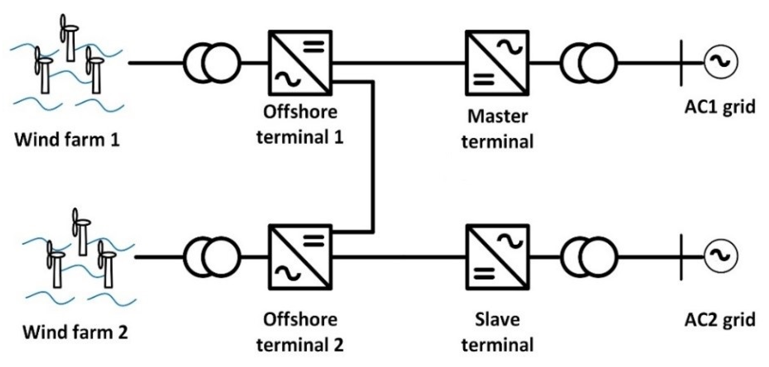
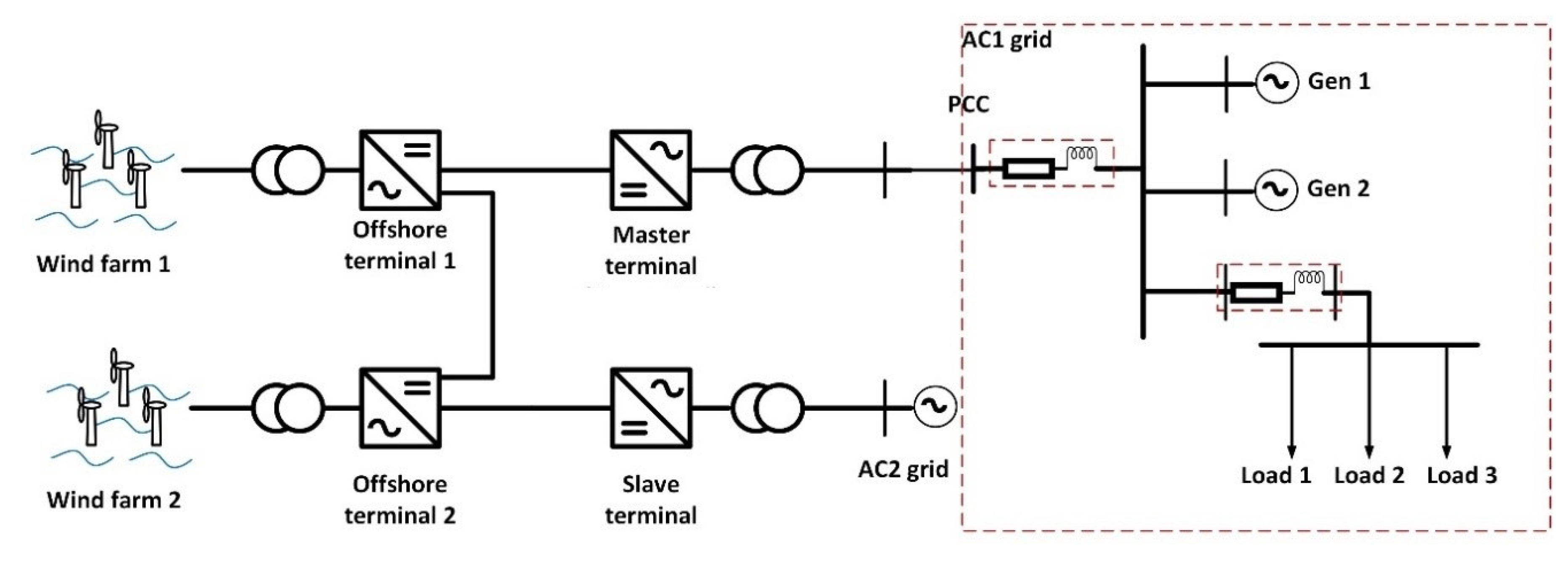
3. Multi-Terminal Direct Current (MTDC) Grid Topology and Control Systems

The MTDC network under study evacuates offshore wind energy to two onshore AC grids and is presented in Figure 1. The MTDC network is composed by 2 onshore (master–slave) and 2 offshore VSC terminals. By means of HVDC links, each offshore VSC terminal is coupled to one onshore VSC terminal and both offshore terminals are coupled at the offshore side. Each HVDC link is made via bipolar HVDC cables with a length of 100 km and a rated voltage and current of 320 kV and 2373 kA, respectively. Each offshore VSC terminal is connected to an offshore wind farm composed by 100 wind turbines of 5.5 MVA each and with a 0.9 inductive-capacitive power factor range.

The HVDC links are also coupled to the onshore AC grid, whose maximum short circuit power is 30,000 MVA and R/X ratio is 0.1.

Average models for onshore and offshore converters can be selected to simulate onshore faults with sufficient accuracy, since the present system is not equipped with fast offshore grid voltage reduction-based fault-ride-through function, as concluded in [22]. Therefore, a modular multilevel converter (MMC) average model is used to model the four terminals of the MTDC grid.

3.1. MTDC Grid Supervisory Control System

Before digging in details of the control systems at terminal level, an overview of the MTDC supervisory control system [7] is given. The MTDC supervisory control is responsible for the distribution of power references within the MTDC grid to convey wind energy from the offshore terminals into the onshore terminals in safe conditions. For this purpose, the role of the exchange mode is to set the DC power reference for the slave terminal, which is a function of the wind energy production coming from the two wind farms, P_WF,1 and P_WF,2, by means of a proportional constant k_PRO, as Equation (1) shows.

$$P_{DC,ref,slave}=k_{PRO}\left(P_{WF,1}+P_{WF,2}\right) 0 p.u.<P_{DC,ref,slave}<P_{nom,slave}$$

(1)

Whenever there is a connection or disconnection event, the distribution of active power will be changed, and the slave terminal will increase or reduce its absorbed active power.

3.2. Control Systems at Terminal Level

At terminal level, the MTDC grid is composed, on the one hand, of two onshore terminals, i.e., the master and slave terminals, which are in charge of controlling the DC voltage and DC power, respectively. On the other hand, it is composed by two offshore terminals that convey the power produced by offshore wind farms.

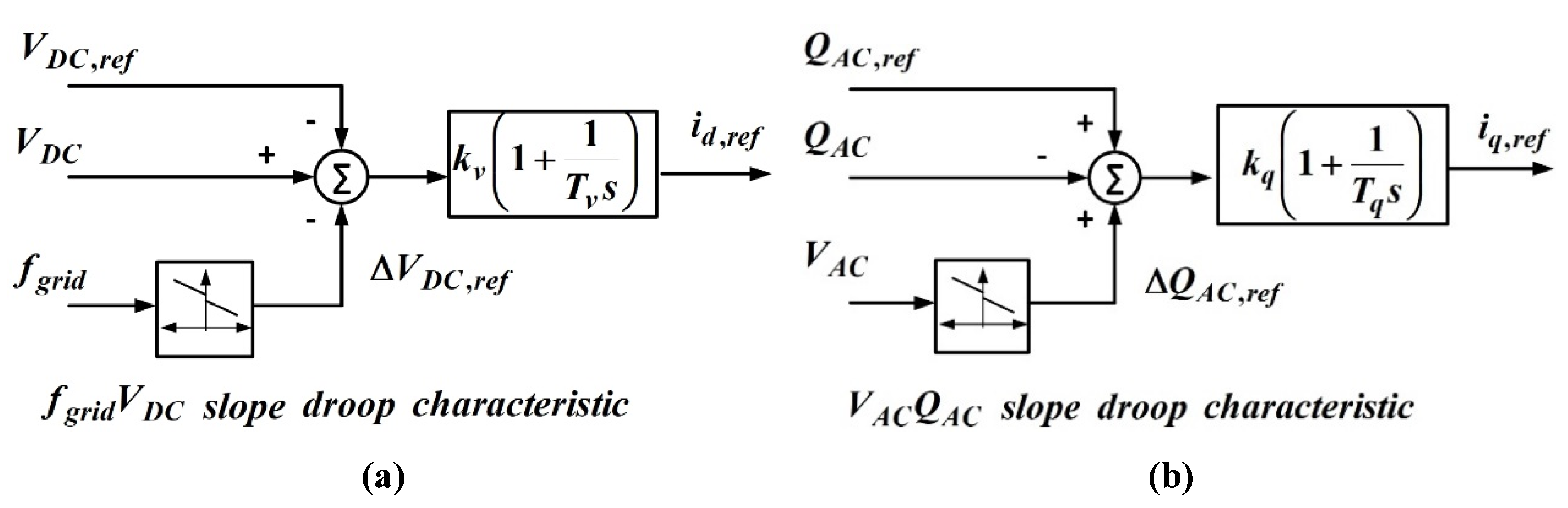
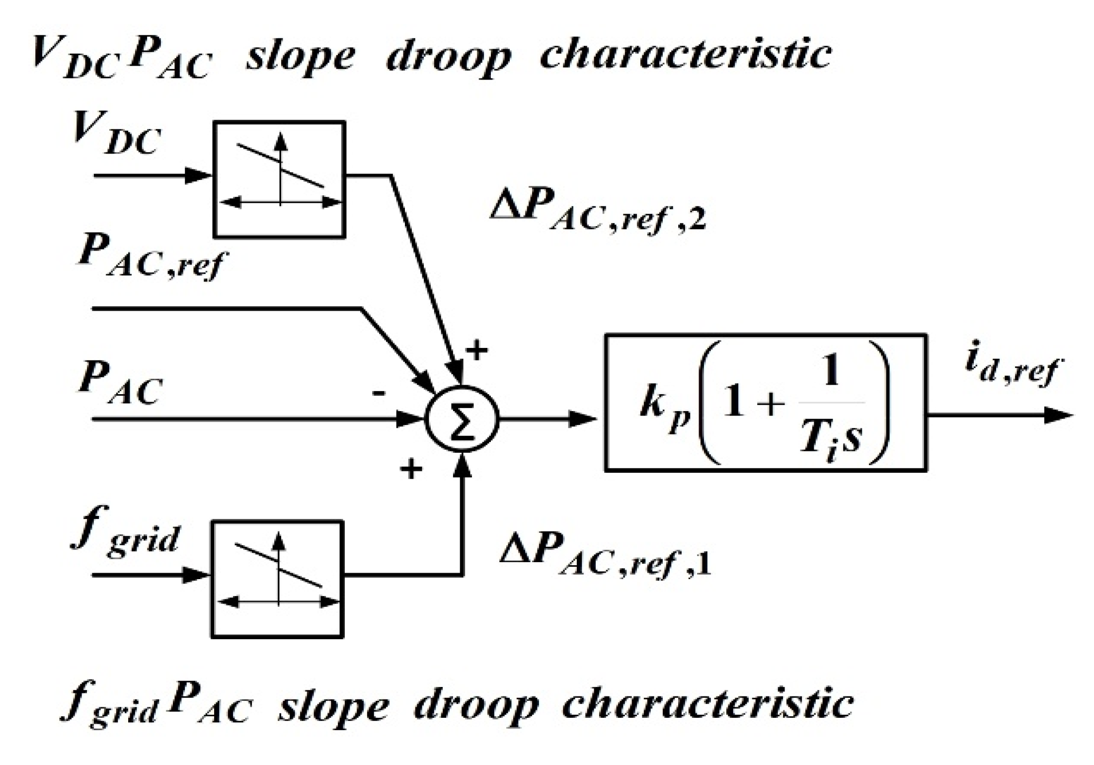
3.2.1. Onshore Terminals

As mentioned previously, being the onshore master terminal responsible for controlling the DC voltage, it uses a V_DCQ scheme. By following this scheme, the DC voltage is controlled by means of i_d,ref (Figure 2a) and includes a f_gridV_DC slope characteristic where the LFSM/FSM frequency-response function is implemented by means of the k_FSM parameter. Besides and according to the V_DCQ scheme, the reactive power is controlled by means of i_q,ref, where a V_ACQ_AC slope droop function is included to contribute to AC voltage stability of the AC grid (Figure 2b).

The onshore slave terminal oversees the active power and includes a f_gridP_AC characteristic where the k_FSM frequency-response function is implemented to comply with the frequency requirements specified in the UK national grid code, as in the master terminal. The slave terminal also contributes to DC voltage stability by means of a droop V_DCP_AC characteristic with dead band around the DC voltage reference. For this purpose, it follows a PQ scheme where the control of reactive power is the same as in the onshore master terminal (Figure 2b). The difference with the master terminal is found at the generation of the i_d,ref, where active power magnitudes are operated instead of DC voltage variables, as shown in Figure 3.

The frequency-response functions in onshore master and slave terminals ensure the LFSM response and FSM modes already described in Section 2. The tuning parameters for achieving these frequency droop loops are equal for both FSM and LFSM modes, thus implying k_FSM = k_LFSM, and for the sake of simplicity k_FSM is used from now on.

Furthermore, both master and slave terminals present the same inner proportional resonant control, already described in [7], and whose control parameters are detailed in Appendix A.

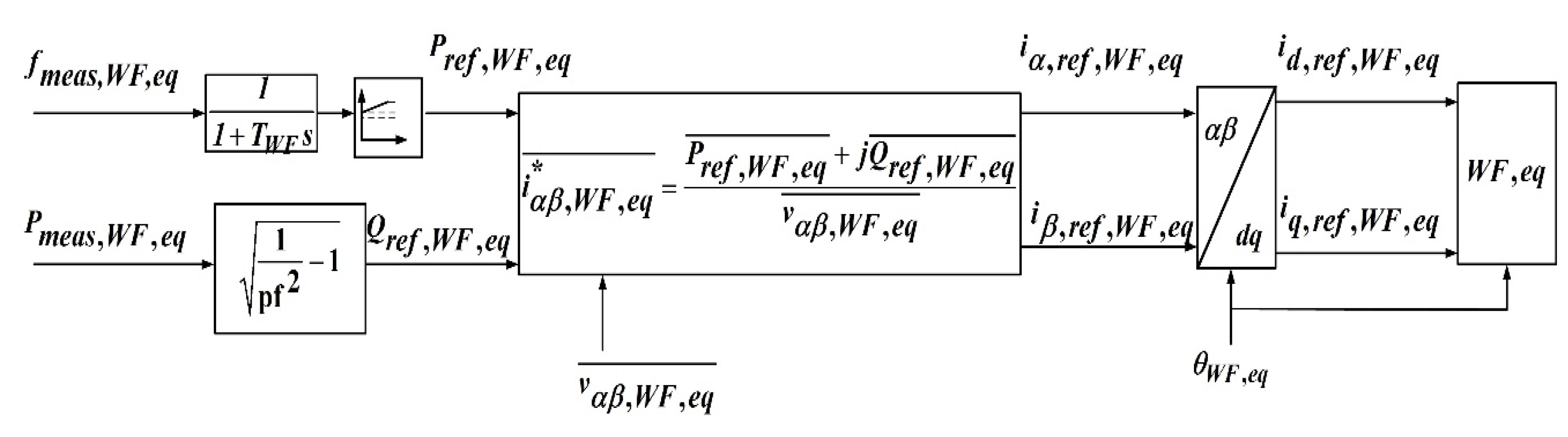
3.2.2. Offshore Terminals

The control scheme of the offshore terminals is depicted in Figure 4. Each offshore terminal has a voltage controller in charge of regulating the amplitude and frequency of the AC voltage at each wind farm. This is done by means of a proportional integral (PI) controller, which obtains the modulation index required by the offshore converter, according to [7]. In order to limit the power generated by the whole farm during DC over-voltages due to contingencies, such as the loss of terminals or DC links, a V_DCf_grid characteristic is added, which allows to modify the wind farm grid frequency, taking advantage of the capability of the wind generators to change their generation against frequency variations.

The control scheme for the offshore terminals is presented in [7], can also be complemented with the control of the offshore wind farm. The offshore wind farms in the present paper follows a control scheme presented in Figure 4, which corresponds to an equivalent wind farm model obtained by a simple aggregation technique. Therefore, the equivalent wind farm model consists in a single wind generator whose apparent power is the apparent power of a single wind generator multiplied by the number of wind generators of the wind farm.

In Figure 4, the frequency and the active power of the aggregated wind farm model, f_meas,WF,eq and P_meas,WF,eq, are measured to calculated the active and reactive power references of the aggregated wind generator, P_ref,WF,eq and Q_ref,WF,eq.

The frequency measurement is first filtered by a first order delay, defined by T_WF, which is aimed at attenuating oscillations provoked by the phase-locked loop (PLL).

For frequency measurements, the PLL is adjusted to have an integral gain of 1 and a proportional gain of 10. Hereupon, the filtered frequency measurement is converted into active power magnitude by means of a f-P droop characteristic. This relates the offshore frequency variations with changes in the wind farm active power. The result of this operation turns to be the active power reference of the aggregated wind farm generator, P_ref,WF,eq.

The active power at the output of the aggregated wind generator is measured to calculate the reactive power reference, Q_ref,WF,eq. Since the offshore wind farms follow a fixed power factor control, the reactive power reference is obtained from the measured active power and the chosen power factor.

The current references in αβ frame, i_α,ref,WF,eq and i_β,ref,WF,eq, are calculated by using the previously calculated, P_ref,WF,eq and Q_ref,WF,eq magnitudes, jointly with the voltage vector, also in αβ frame, measured at the output of the aggregated wind farm generator, $\overline{v_{\alpha \beta ,WF,eq}}$. According to the operation shown in Figure 4, the current references in the αβ frame are transformed into dq frame by means of the Park transform, considering the angle measured by the PLL, θ_WF,eq.

Finally, the aggregated wind farm generator is controlled by the dq current references, i_d,ref,WF,eq and i_q,ref,WF,eq, and the θ_WF,eq angle.

The aggregated wind-farm generator is modelled as a static generator and this implies that no dynamic functions of the wind turbines are included. This approach has been justified previously as adequate in the literature for the case of wind farms connected by means of an HVDC link [22], since the present study only deals with onshore faults. If offshore faults were considered, a more detailed wind turbine model would be necessary.

4. Open-Loop Frequency Response of the MTDC Grid

The control structure presented in Section 3 has been tested against the set of frequency steps recommended by the UK national grid code to validate the behaviour of the system under frequency excursions. This test is specified for testing the frequency response of power park modules and offshore transmission system user [19]. This test should be programmed when 95% of the power park units within a power park module is in service, according to [19], where the terms designed as power park units and module are properly defined. Furthermore, the simulated frequency deviations should be applied into the frequency controller reference summing junction, when the frequency controller is in FSM or LFSM mode [19]. In addition to this, the ability of the power park module to deliver a requested steady-state power output needs to be demonstrated [19].

In Figure 5, the frequency signal measured at the PCC and the power absorbed from the master terminal (ΔP_DC (p.u.)) are shown as a final proof of compliance with the frequency response. Different settling times have been obtained to reach set points of 10 s and 30 s as well as holding times of 20 s to maintain the frequency at a constant value at several stages of the sequence. The simulation results show that the proposed control structure is compliant with the grid code requirements.

In Figure 5, the green line corresponds to the level of 50 Hz and detailed information of the events can be consulted in [19].

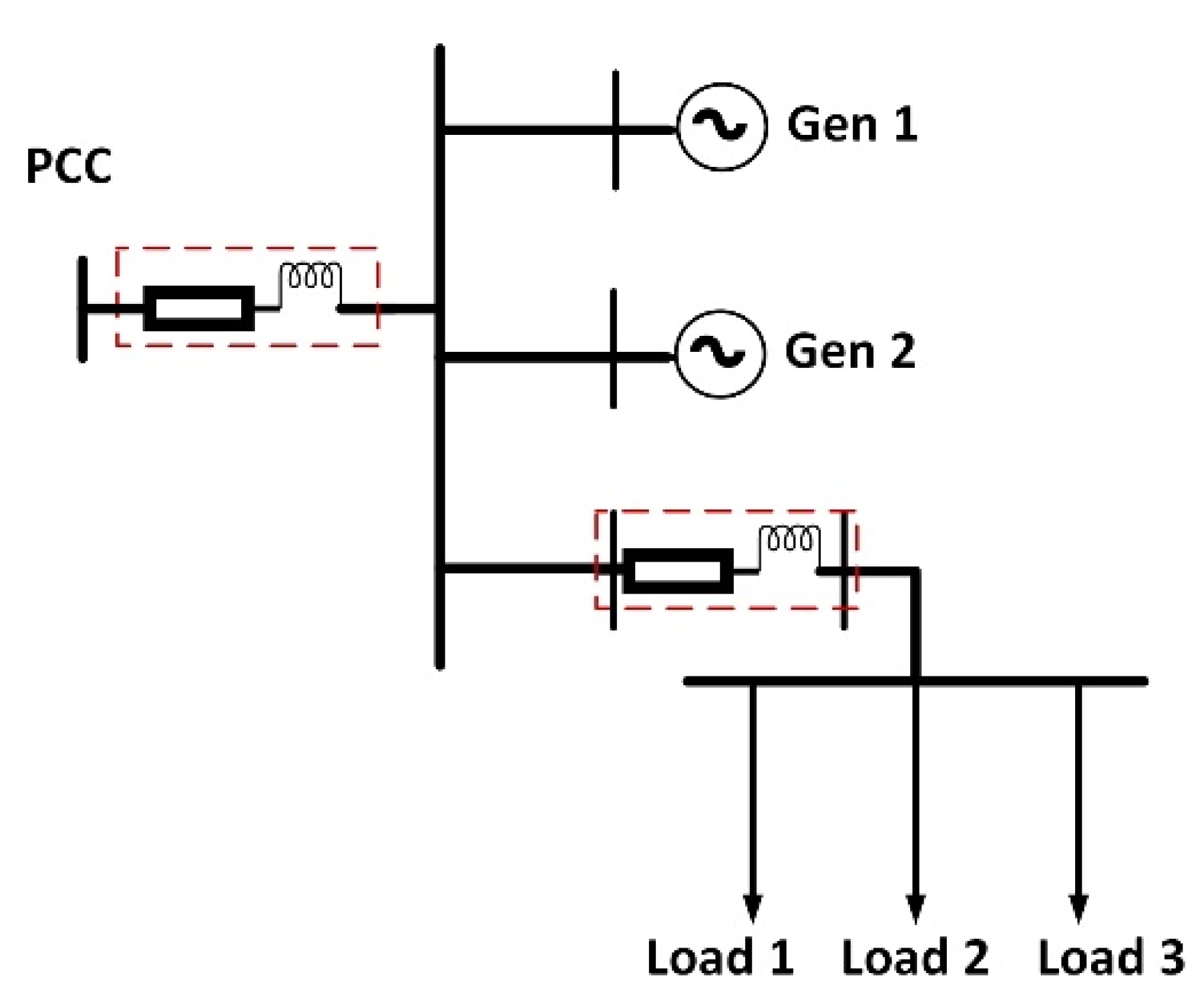
5. Onshore Alternating Current (AC) Grid Model to Emulate Frequency Response

The test performed in Section 4 is an open-loop validation of the control against simulated frequency variations. In order to analyse the closed-loop response, additional validation tests are needed. In several countries, compliance with grid code requirements is allowed to be evaluated by computer simulations, provided that the simulation models of the generating units are validated with real measurements during tests [1]. This happens, for example in Germany and Spain with the FGW-TG3 and the response of wind farms in the event of voltage dips (PVVC) procedure, respectively, according to [1]. For that purpose, in the literature frequency events have been introduced by random load increase or decrease events [15,16,23], random generation loss events for the study of under-frequency response [24,25], or by power system models such as the 3-bus great britain (GB) model and the simplified GB model in [26].

In the present paper, these disturbances will be introduced at the PCC of the onshore grid (AC1 in Figure 6), replaced by an equivalent grid model parameterised for specific frequency events, with identical short-circuit power. The topology of this equivalent model is shown in Figure 6.

The PCC point shown in Figure 6 corresponds to the point of common coupling between the onshore master terminal and the AC1 grid corresponding to Figure 1.

The model is based on a SFR model, which represents an aggregate load-frequency behaviour following load-generation unbalance [27]. With the equivalent grid model, an under-frequency event can be emulated by the connection of an additional load (Load 3 in Figure 6) or the disconnection of a small generator (Gen 2 in in Figure 6). Therefore, a deficit in generation and excess of demand will be observed and an under-frequency event will occur. By contrast, an over-frequency event can be emulated by a partial load shedding (Load 2 in Figure 6, or by the connection of a small generator (Gen 2 in in Figure 6). This imposes an excess of generation and a deficit of demand, resulting in an over-frequency event. The inertia constant of the equivalent power system is represented by a single generating unit (generator Gen 1 in Figure 6), where a simplified first-order governor and excitation system models are used, based on [28].

Hence, several of the onshore grid model characteristic depend on the frequency event to emulate. Thus, a wide range of events can be simulated. By parameterising the equivalent model, frequency events can be simulated with specific frequency characteristics of rate-of-change-of-frequency (ROCOF), minimum/maximum frequency value (frequency nadir) and frequency deviation in steady-state. All three magnitudes can be calculated by using Equations (2)–(4), respectively. The adjustment is based on an active power mismatch ΔP₀, which will be a generation trip for under-frequency events and a load trip for over-frequency events.

In a power system with multiple generators, when part of the generation is lost, system frequency starts to drop. Assuming that all generators remain in synchronism, they slow down at approximately the same ROCOF as indicated in Equation (2).

$$\Delta P_0=2{\displaystyle \sum }_{i=1}^n\frac{H_i{S}_i}{S_T}ROCOF=2H_{eq}ROCOF$$

(2)

In Equation (2), ΔP₀ is the active power mismatch, H_i, and S_i the inertia constant and the apparent power of the individual generators making up the system, S_T the total capacity in the system and H_eq the equivalent inertia of the system. The computation of frequency deviation in the steady-state value in a power system with several generators is also straightforward by applying Equation (3).

$$\Delta P_0=\left({\displaystyle \sum }_{i=1}^n\frac{1}{R_{droop,i}}+D_t\right)\Delta f_{ss}=\left(\frac{1}{R_{droop,eq}}+D_t\right)\Delta f_{ss}$$

(3)

In Equation (3), R_droop,i is the droop constant of the individual generators making up the system, D_t, the damping constant in the system, and R_droop,eq the equivalent droop constant in the system.

The calculation of the minimum frequency after an active power mismatch depends on the frequency-response strategies of the network assets, such as conventional generating units, renewable generating units, storage systems or demand assets. Therefore, the equivalent SFR model results in a complex function dependent on several variables. Consequently, several authors have introduced simplifying hypotheses in order to compute frequency response in a power system [22,23].

In the present case, the equivalent power system is represented by a single generating unit with a simplified first-order governor and excitation system model. Therefore, the adjustment for the frequency minimum/maximum value results in Equation (4):

$$\Delta P_0=\Delta f_{min}\frac{D_t+K_{eq}}{1+\frac{e^{-\varsigma {\omega }_n{t}_{min}}}{\sqrt{1-{\varsigma }^2}}\left(T_{eq}{\omega }_{n}sin\left({\omega }_r{t}_{min}\right)-sin\left({\omega }_r{t}_{min}+{\theta }_1\right)\right)}$$

(4)

In Equation (4), ω_r, ω_n, ζ, and θ₁ can be calculated based on [16] and considering a first-order system. K_eq and T_eq are respectively the gain and time constant of the first-order governor in Gen 1 and t_min is calculated with Equation (5):

$$t_{min}=\frac{1}{{\omega }_r}atan\frac{{\omega }_n{T}_{eq}\sqrt{1-{\varsigma }^2}}{{\omega }_n{T}_{eq}\varsigma -1}$$

(5)

The values of the control parameters for the onshore AC grid model are summarised in Appendix A.

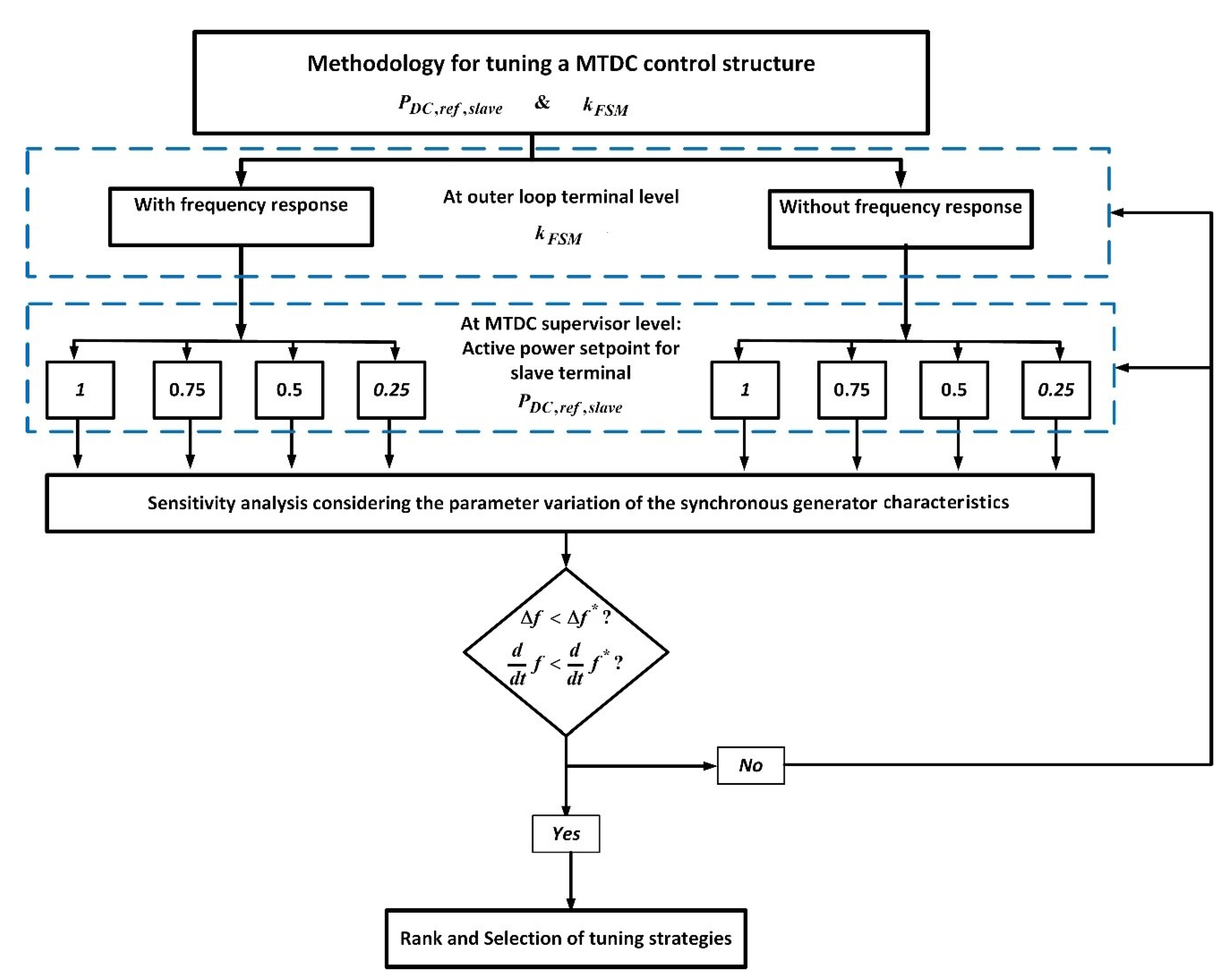
6. Novel Methodology to Tune MTDC Supervisory and Frequency-Response Control Functions at Terminal Level in Over-Frequency Events

In this section the novelty of the present paper is described, i.e., the methodology to tune jointly the supervisory and frequency-response control functions of outer loops at terminal level. In Figure 7, the complete system of the MTDC grid connected to the onshore AC grid model is depicted. This contains the MTDC grid, described in Section 3, connected to the onshore AC grid model to simulate the frequency events applied at the PCC point shown in Figure 7.

In Figure 8, a flowchart of the methodology, applied to the system in Figure 7, is exposed, where the supervisory control and the frequency-response functions of the onshore terminals are two major aspects to define the tuning strategies in order to obtain reductions in the frequency peak. Besides, for certain levels of k_FSM value, even the order type of the frequency signal may be reduced from 2nd order to 1st order.

Therefore, the flowchart in Figure 8 allows two control levels of the hierarchical MTDC coordinated control structure to be tuned simultaneously.

On the one hand, it allows the MTDC supervisory control to be tuned, by means of choosing the proper active power exchange set point (from now on, P_DC,ref,slave). The values tested for P_DC,ref,slave have been selected according to four equal shares of the maximum capacity of the slave terminal.

On the other hand, it allows the outer loop control of onshore terminals to be parameterised by means of setting the proper slope for the frequency response (k_FSM). The values that k_FSM adopts are chosen among those recommended by the UK national grid code [19,20] (3–5%), and even trying greater values such as 7.5% to check for further improvements.

The definition of tuning strategies is detailed in

Table 1. Definition of tuning strategies according to k_FSM and P_DC,ref,slave.

Strategies	kFSM	PDC,ref,slave
Strategy 1	0%	0.25	0.5	0.75	1
Strategy 2	5%
Strategy 3	7.5%

, where the values for both P_DC,ref,slave and k_FSM are clarified.

These tuning strategies are aimed at reducing the frequency peak at the PCC of the onshore AC grid. Indeed, the proper combination of both P_DC,ref,slave or the k_FSM values can also transform the 2nd order nature of the frequency excursion into a 1st order nature.

Furthermore, the sensitivity of the tuning strategies must be checked against variations in the parameters of the synchronous generator, such as the equivalent inertia or damping. According to this sensitivity analysis, the peak of frequency will also experience changes and therefore, the optimal strategy may vary.

If the frequency peak is not sufficiently smoothed by a strategy for a specific case, then P_DC,ref,slave or the k_FSM values can be readjusted and reductions of the frequency peak at PCC can be checked. For this purpose, a threshold value for frequency can be selected and the established limit for the LFSM band, i.e., 50.4 Hz, is proposed. In this way, this limit bounds the frequency signal out of the LFSM compulsory band, and therefore, the risk of instability is reduced.

Each of the strategies can be ranked upon the reduction of maximum frequency peak they can achieve. Therefore, most of the novelty of the proposed methodology is based on the implication of different control levels jointly for proper tuning of the control structure and the verification of the improvements by means of maximum frequency peak reductions.

7. Application Case of the Methodology to the Considered MTDC + Onshore AC Grid

The methodology proposed in the present paper is applied to a case study consisting in the system presented in Figure 7, by means of electro-magnetic transient (EMT) simulations carried out in DIgSILENT PF software. (Version 2019 SP3 (x64), DIgSILENT GmbH, Gomaringen, Germany) This system is tested under constant wind energy production, where each wind farm produces 400 MW.

For this purpose, the coordinated control structure is tested against frequency excursions using the AC grid equivalent model introduced in Section 5. The control parameters selected for both MTDC and onshore AC grid are detailed in Appendix A. A short-circuit ratio of 20.5 measured at the PCC has been considered. The analysed system consists of two loads of 890.5 MW and 250 MW, Load 1 and Load 2 respectively, as shown in Figure 7. When the 250 MW load is disconnected, an over-frequency deviation (>50.4 Hz) is observed at the PCC, making the system work under the LFSM frequency band. The system enters the over-frequency FSM band by disconnecting Load 2 in Figure 7. In this case, 120 MW is the load value considered to disconnect, since the provoked frequency excursions are within FSM bonds, i.e., lower than 50.5 Hz and higher than 50.015 Hz in case of over-frequency.

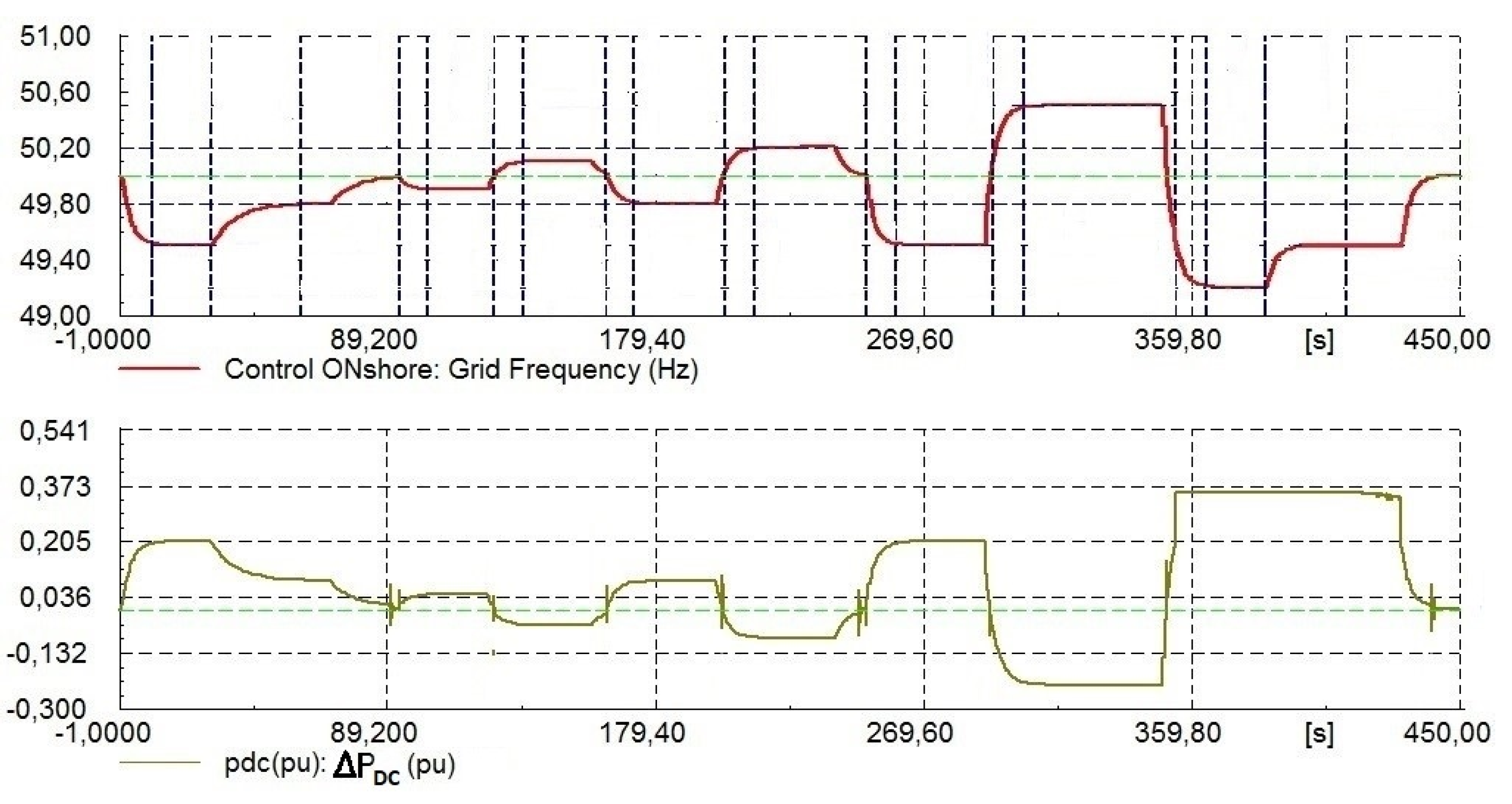
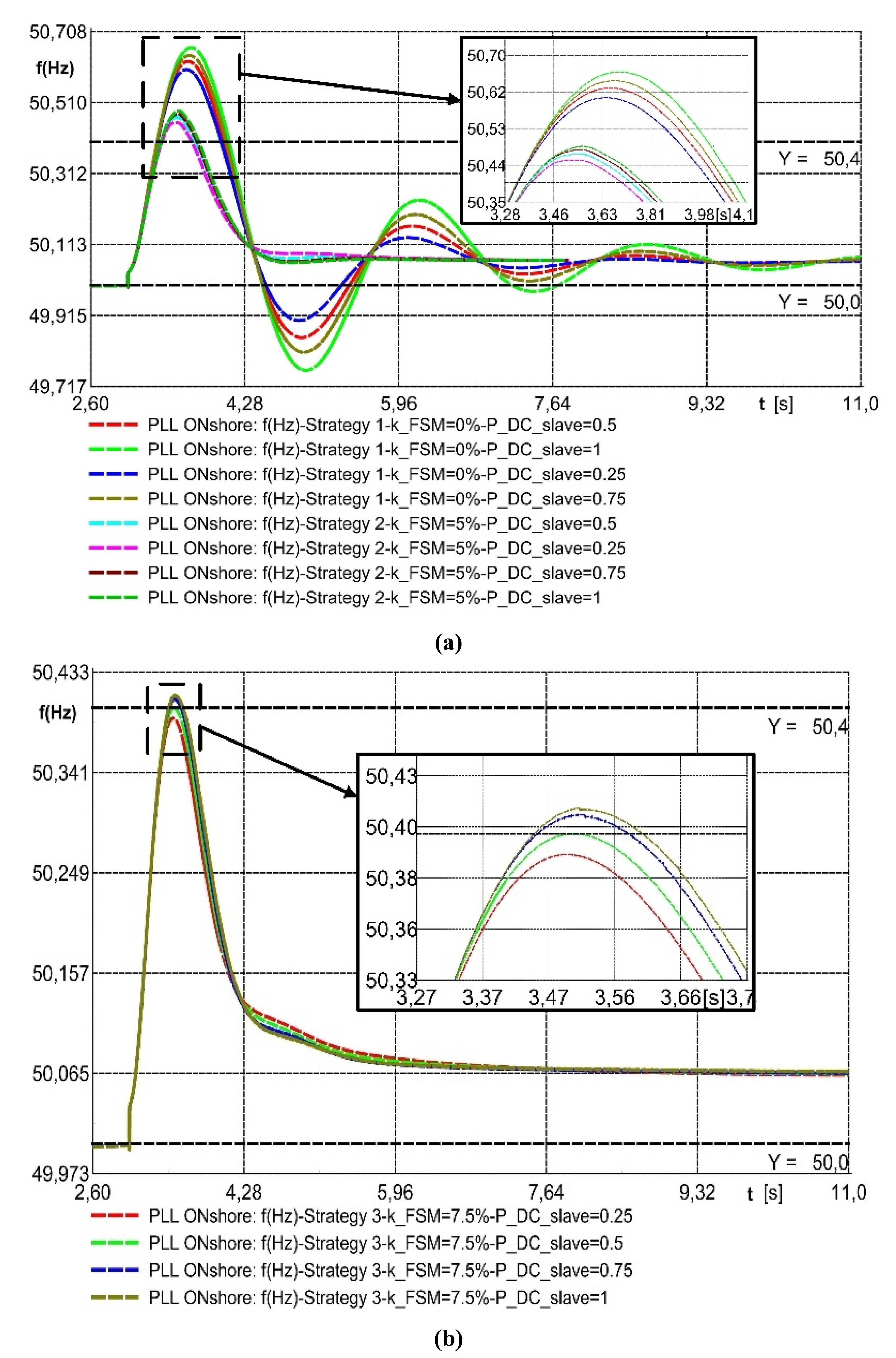
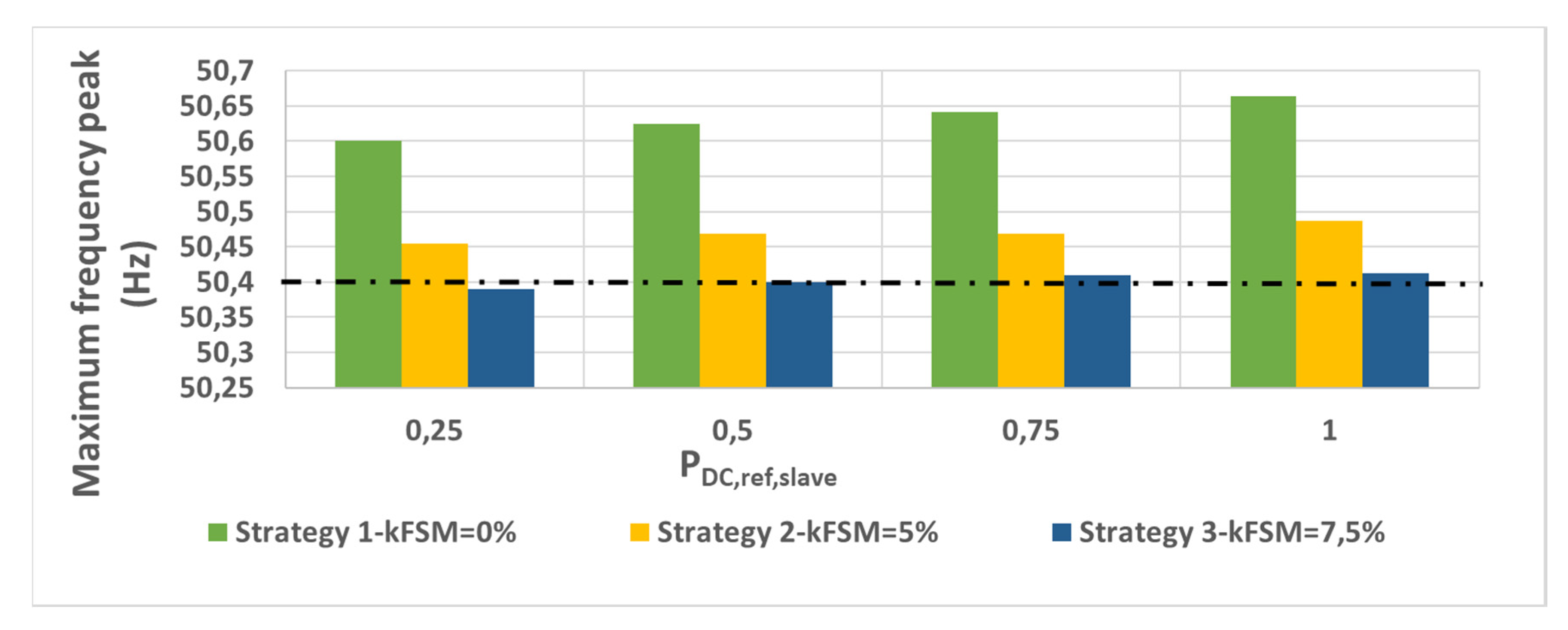
7.1. Impact of Tuning Strategies on the Reduction of the Frequency Peak

The benefit of implementing a frequency response at onshore terminal level, i.e., the reduction of transient frequency oscillation amplitude, is shown Figure 9a,b, by means of the implementation of different tuning strategies according to Table 1.

In Figure 9a, the reduction of the frequency peak value when a frequency-response function is implemented, namely k_FSM = 5% (strategy 2) can be observed with respect to the original system without frequency-response function, i.e., k_FSM = 0% (strategy 1). Both tuning strategies are parameterised according to different P_DC,ref,slave values, in order to further reduce the peak value in a more moderate manner than with the change of k_FSM, so that the lowest P_DC,ref,slave value yields to the greatest peak frequency reduction.

Furthermore, in Figure 9a, the inclusion of the frequency-response function not only reduces the frequency peak, but also changes the frequency curve order from second-order type with k_FSM = 0% to first-order type with k_FSM = 5%. An intermediate value of k_FSM = 3% has been also simulated and this presents a second-order type, but for the sake of clarity it has been removed from Figure 9a. The k_FSM = 5% is the limit value up to which the frequency curve is a second-order type. For larger values, such as k_FSM = 7.5%, the first order type curve is still maintained and further greater reductions in the frequency peak are shown, as depicted in Figure 9b.

Therefore, both P_DC,ref,slave and k_FSM variables contribute to this peak reduction slightly and more considerably, respectively, being k_FSM even capable of changing the polynomial order type of the frequency signal and P_DC,ref,slave values able to slightly modify the final peak value derived from k_FSM variation.

In Figure 10, the reductions in frequency peak among strategies are compared by taking into account the P_DC,ref,slave values. The greatest improvements in frequency peak are observed for strategy 3 with k_FSM = 7.5% and P_DC,ref,slave = 0.25, reaching 50.39 Hz, and the worst case is observed for strategy 1 with P_DC,ref,slave = 1, reaching 50.66 Hz, as seen in Figure 10.

If the strategies are compared within the same k_FSM value, one can distinguish that for 0, 5 and 7.5%, the greatest P_DC,ref,slave value leads to the largest frequency peak value. Therefore, those strategies which employ high P_DC,ref,slave set points lead to worst case scenarios for a given k_FSM. This can be especially observed in frequency peak reduction provided by strategy 1, which presents the greatest improvements made by P_DC,ref,slave values from all the selected cases, as the target variables are reduced more drastically when P_DC,ref,slave is decreased from 1 to 0.25.

If the strategies are compared within the same P_DC,ref,slave set point value, greater reductions in frequency peaks are obtained as far as k_FSM is increased. Moreover, several P_DC,ref,slave values achieve in strategy 3 frequency peak values lower than 50.4 Hz, namely, P_DC,ref,slave = 0.25 and P_DC,ref,slave = 0.5. These combinations ensure that the complete frequency signal is out of the LFSM compulsory zone, where mandatory extra frequency response should be added if frequency values greater than 50.4 Hz are maintained.

The benefits of having implemented the combined effects of both k_FSM and P_DC,ref,slave values correspond to a case where an optional FSM ancillary service would be contracted. When the frequency-response function is contracted with the electrical utility as an ancillary service, several considerations must be addressed. In [29], a typical frequency response for a synchronous area under frequency disturbances for effective primary control is shown. In [29], the response is exemplified with an under-frequency event where the transient behaviour is characterised by oscillations and a time response from 15 s to 30 s. Therefore, it is important to test these reductions for a certain variation of the synchronous generator parameters. Among tuning strategies, strategy 2 (k_FSM = 5%) is chosen due to its intermediate reduction of the frequency peak and being k_FSM = 5% a limit value for the first-order behaviour of the frequency curve at PCC.

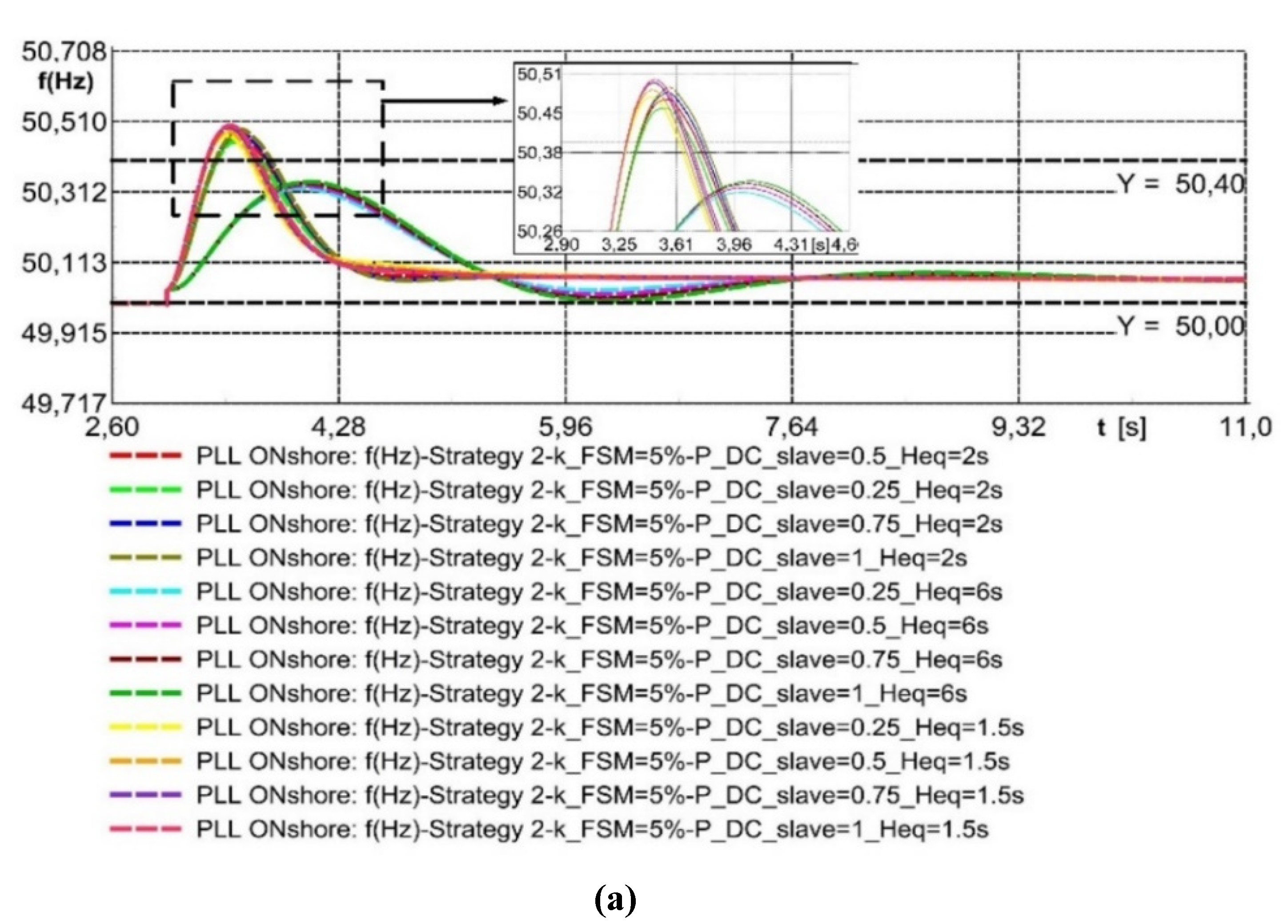
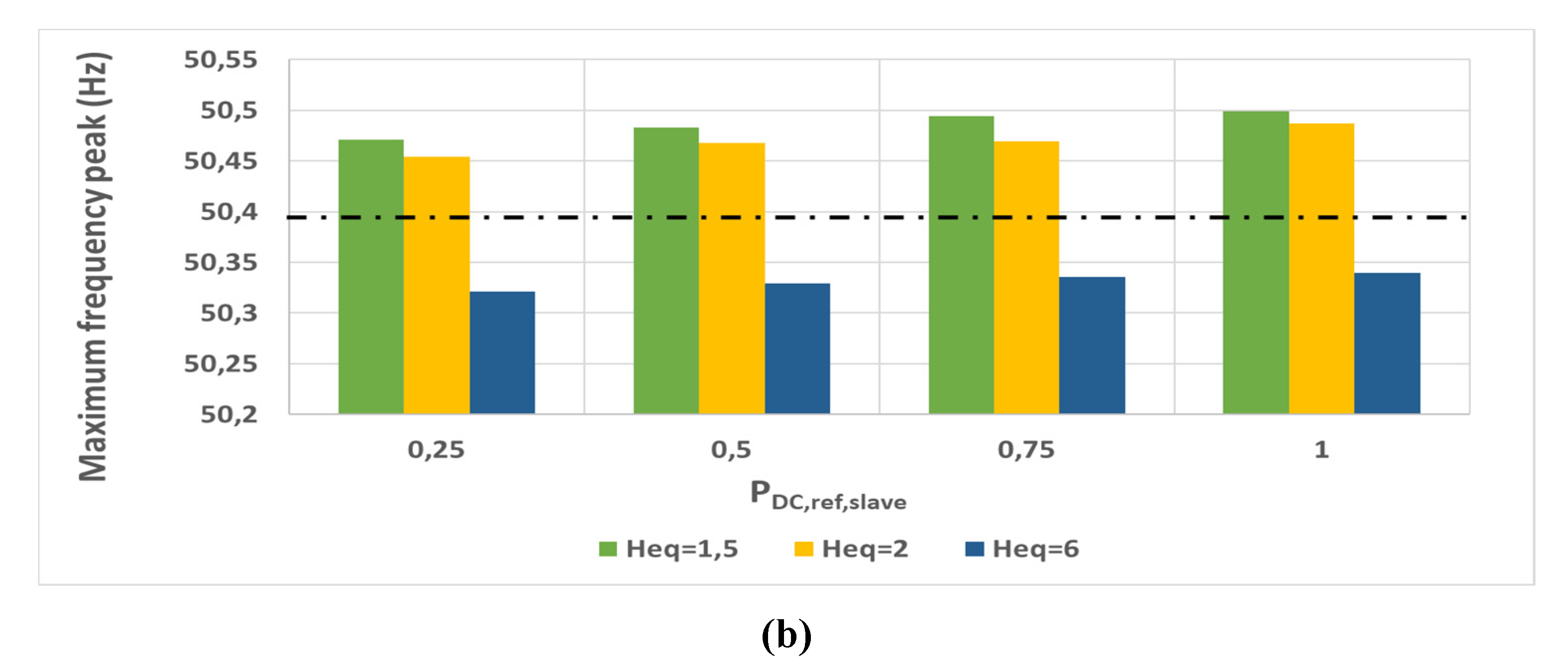
7.2. Guidance for Tuning k_FSM and P_DC,ref,slave when Different MTDC Control Structure and Synchronous Generator Characteristics Are Considered

In this Section, the frequency peak reduction is analysed within a specific strategy chosen from the previous analysis conducted in Section 7.1. The main objective of this Section is to give systematic guidance for adjusting the two control-level parameters, k_FSM and P_DC,ref,slave, when the control structure of the MTDC grid is varied, i.e., instead of master–slave, a distributed control scheme, or the onshore AC grid characteristics are modified.

Strategy 2, while encompassing the whole range of P_DC,ref,slave, implies a moderate tuning of the frequency-response function, k_FSM = 5%, of onshore terminals.

According to CC.6.3.7(c)(ii) in [19,20], the k_FSM for the LFSM mode has to be at least 2% per each 0.1 Hz. In principle, for those frequency ranges that belong to the LFSM band there would be no problem since, k_FSM = 7.5% exceeds this recommended minimum slope of 2% per each 0.1 Hz. However, for those frequency values belonging to the FSM band, the recommended k_FSM value lays between 3% and 5% per each 0.1 Hz, as reported in [20]. By contrast, these boundaries for k_FSM within the FSM band are neither justified in the grid code [19] nor in the guidance note for DC converter stations [20].

To the best knowledge of the authors, k_FSM = 7.5% could imply a bit aggressive control, considering that the FSM frequency range is narrower than the LFSM range. Moreover, although not considered in this paper, k_FSM can also present an opposite sign, as it should also consider under-frequency values with respect to 50 Hz. However, this could be more critical for a more complex distributed frequency control structure with a specifically located centre of inertia; nevertheless, the present paper considers a hierarchical master–slave structure. Therefore, more moderate values of k_FSM are recommended for distributed control structures than in master–slave structures, while P_DC,ref,slave can be varied for the entire range, as it conducts to lower peak reductions or just peak amendment.

As for the onshore AC grid characteristics, several parameters of the main synchronous generator of the onshore AC grid are varied to extract guidelines on how to tune jointly the MTDC supervisory and outer loop frequency-response functions. According to the previous discussion, a moderate k_FSM value is recommended and thus strategy 2 of Table 1 has been chosen. Therefore, strategy 2 is selected to be evaluated against a variation of the Gen 1 synchronous generator characteristics, such as the total inertia, H_eq, and the damping, D_t, according to Equations (2)–(4). Strategy 2 is tested against a variation of H_eq, adopting the values of 1.5 s, 2 s and 6 s, and the impact on the frequency peak is shown in Figure 11a.

In Figure 11a, the H_eq = 6 s conducts to the slowest set of curves as well as the greatest reductions (50.32 Hz with P_DC,ref,slave = 0.25), while H_eq = 1.5 s conducts to the fastest profiles and smaller reductions of the peak (50.49 Hz with P_DC,ref,slave = 1).

According to Figure 11b the P_DC,ref,slave values also contribute to the decrease of the peak values, as far as they are reduced. The H_eq = 6 s value yields to frequency values out of the compulsory LFSM zone since the peak values are lower than 50.4 Hz. This strategy would ensure that the complete frequency signal is out of the LFSM compulsory zone, where mandatory extra frequency response should be added if frequency values greater than 50.4 Hz are maintained.

Therefore, for H_eq values close to 6 s, it may be sufficient to tune P_DC,ref,slave values to smooth the peak and ensure the frequency signal outside the LFSM range. In contrast, for H_eq values close to 1.5–2 s, the curves are transiently inside of the LFSM zone, but getting out of this area thanks to the frequency-response function. Therefore, for large H_eq values, a smaller k_FSM value than 5% could also provoke reductions in the peak, while P_{DC,ref, slave} is kept to a minimum. For lower H_eq values, a substantially greater k_FSM value would be needed, in order to achieve greater peak reductions.

As for the sensitivity against the variation of D_t, the complete model has been tested when D_t adopts the values of 0, 1.25 and 2.5, which would lead to a system without and with damping, respectively. In Figure 12a, the effect of these variations on the frequency behaviour is shown, and in Figure 12b, the peak values are compared.

In Figure 12a, two sets of curves are derived, one corresponding to D_t = 0, with the greatest peak values, and another with D_t = 2.5, leading to peak reductions. Apart from this, the decrease of the P_DC,ref,slave values contribute to the peak reduction. With D_t = 2.5, the frequency peak is outside the LFSM compulsory area when the P_DC,ref,slave value equals to 0.25.

Therefore, for a null D_t value, a greater k_FSM value than 5% has a great influence in achieving peak reductions in a more efficient way than P_{DC,ref, slave}. However, for greater D_t values, just by maintaining a low P_{DC,ref, slave} value, the peak reduction is easily obtained, without the need for increasing the k_FSM slope.

Therefore, with the proper combined tuning of P_DC,ref,slave and k_FSM values, the peak of the frequency signal can be further reduced in a slight and a more considerable manner with the proper combination of k_FSM and P_DC,ref,slave values, respectively. Additionally, the complete frequency curve can be fully bounded outside the LFSM area, reducing the risk of the system to instability. This also is applicable when a certain variation of the onshore grid synchronous generator characteristics is simulated.

8. Conclusions

The main innovation of this paper is the development of a methodology for tuning simultaneously two hierarchical levels of a MTDC coordinated control structure, i.e., the MTDC supervisory, given by the active power set point for the slave terminal P_DC,ref,slave, and the slope of the frequency-response functions in outer loop control schemes of onshore terminals, k_FSM.

The MTDC control structure has been first validated in open-loop configuration by applying the recommended set of frequency steps by the UK national grid code, showing robustness of operation. It can be extracted from a previous test whereby both MTDC coordinated frequency control and onshore AC equivalent grid control schemes interact with oscillatory behaviour typical from primary control response with a settling time between 2 s and 25 s and by always respecting the grid code limits.

As for the methodology, several conclusions can be obtained from the previous analysis carried out in the above sections.

• First, the combination of a coordinated frequency control structure with a centralised master–slave scheme to operate a MTDC grid implemented to ensure the proper share the distribution of power set points, while at the same time, comply with the considered grid code.
• The comparison between control responses with and without this k_FSM frequency-response function shows the benefit of having it implemented, i.e., the reduction of transient frequency oscillation amplitude.
• The strategies which use P_DC,ref,slave = 1 are less preferable than those with P_DC,ref,slave < 1, but can also achieve great frequency peak and slope reductions if an adequate k_FSM is tuned.
• The DC power reference for the slave terminal plays an important role in smoothing the frequency peak value but the role of k_FSM at terminal level has a larger influence in reducing the frequency peak value.
• For a given DC power reference at the slave terminal, a higher k_FSM, e.g., 5%, is advised over lower values, and this guarantees the stability of the system at each moment and presents first order behaviour; or even 7.5%, as it bounds the frequency signal out of the LFSM compulsory area for certain P_DC,ref,slave values.
• For a given k_FSM value, it is advisable to have the lowest P_DC,ref,slave value at the slave terminal, as 0.25 was demonstrated to be the set point which most reduces the frequency peak.
• Besides, guidance is given on how to select the k_FSM value, if the control structure of the MTDC grid is changed. If, for example a distributed control structure was considered, more moderate values for k_FSM are recommended.
• Additionally, a sensitivity analysis is performed to give guidance on how to tune P_DC,ref,slave and k_FSM, considering variations in the equivalent inertia H_eq and the damping, D_t. According to these deviations, the frequency peak values may vary, and thus the strategies have to be redefined if their derived peak reduction is not sufficient. Therefore, for large H_eq values, a smaller k_FSM value than 5% could also provoke reductions in the peak, while P_{DC,ref, slave} is kept to a minimum. For lower H_eq values, a substantially greater k_FSM value would be needed, in order to achieve greater peak reductions. Furthermore, for a null D_t value, a greater k_FSM value than 5% has a great influence in achieving peak reductions in a more efficient way than P_{DC,ref, slave}. However, for greater D_t values, just by maintaining a low P_{DC,ref, slave} value, the peak reduction is easily obtained, without the need for increasing the k_FSM slope.

It has been demonstrated through the FSM frequency droop function, that the MTDC link that conveys offshore wind energy into the onshore grid can act as an ancillary service in the case of onshore frequency excursions, by giving support through its coordinated frequency control.

References

1. Etxegarai, A.; Eguia, P.; Torres, E.; Buigues, G.; Iturregi, A. Current procedures and practices on grid code compliance verification of renewable power generation. Renew. Sustain. Energy Rev. 2017, 71, 191–202. [Google Scholar] [CrossRef]
2. ENTSOE. High Voltage Direct Current Connections. Available online: https://www.entsoe.eu/network_codes/hvdc/ (accessed on 14 April 2020).
3. Fein, F.; Borecki, J.; Groke, H.; Orlik, B. Decentral control of multi-terminal HVDC systems with automatic exchange of instantaneous and primary reserve power across AC grids. In Proceedings of the 2015 17th European Conference on Power Electronics and Applications (EPE’15 ECCE-Europe), Geneva, Switzerland, 8–10 September 2015; pp. 1–8. [Google Scholar]
4. Andreasson, M.; Wiget, R.; Dimarogonas, D.V.; Johansson, K.H.; Andersson, G. Distributed primary frequency control through multi-terminal HVDC transmission systems. In Proceedings of the 2015 American Control Conference (ACC), Chicago, IL, USA, 1–3 July 2015; pp. 5029–5034. [Google Scholar]
5. Cao, J.; Du, W.; Wang, H.F.; Bu, S.Q. Minimization of Transmission Loss in Meshed AC/DC Grids with VSC-MTDC Networks. IEEE Trans. Power Syst. 2013, 28, 3047–3055. [Google Scholar] [CrossRef]
6. Nanou, S.; Tzortzopoulos, O.; Papathanassiou, S. Evaluation of DC voltage control strategies for multi-terminal HVDC grids comprising island systems with high RES penetration. In Proceedings of the 11th IET International Conference on AC and DC Power Transmission, Birmingham, UK, 10–12 February 2015; pp. 1–7. [Google Scholar]
7. Larrode, M.H.; Temez, Í.V.; Recio, S.C.; Mugica, M.S.; Lopez, P.E. Integral control of a Multi-Terminal HVDC-VSC transmission system. In Proceedings of the 2017 Twelfth International Conference on Ecological Vehicles and Renewable Energies (EVER), Monte Carlo, Monaco, 11 April 2017; pp. 1–15. [Google Scholar]
8. Haileselassie, T.M.; Uhlen, K. Primary frequency control of remote grids connected by multi-terminal HVDC. In Proceedings of the IEEE PES General Meeting, Montreal, QC, Canada, 2–6 August 2010; pp. 1–6. [Google Scholar]
9. Zeni, L.; Morgans, I.; Hansen, A.D.; Serensen, P.E.; Kjœr, P.C. Generic models of wind turbine generators for advanced applications in a VSC-based offshore HVDC network. In Proceedings of the 10th IET International Conference on AC and DC Power Transmission (ACDC 2012), Birmingham, UK, 4–5 December 2012; pp. 1–6. [Google Scholar]
10. Phulpin, Y. Communication-Free Inertia and Frequency Control for Wind Generators Connected by an HVDC-Link. IEEE Trans. Power Syst. 2012, 27, 1136–1137. [Google Scholar] [CrossRef]
11. Sakamuri, J.N.; Altin, M.; Hansen, A.D.; Cutululis, N.A.; Rather, Z.H. Coordinated control scheme for ancillary services from offshore wind power plants to AC and DC grids. In Proceedings of the 2016 IEEE Power and Energy Society General Meeting (PESGM), Boston, MA, USA, 17–21 July 2016; pp. 1–5. [Google Scholar]
12. Silva, B.; Moreira, C.L.; Seca, L.; Phulpin, Y.; Lopes, J.A.P. Provision of Inertial and Primary Frequency Control Services Using Offshore Multiterminal HVDC Networks. IEEE Trans. Sustain. Energy 2012, 3, 800–808. [Google Scholar] [CrossRef]
13. Sanz, I.M.; Chaudhuri, B.; Strbac, G. Inertial response from offshore wind farms connected through DC grids. In Proceedings of the 2016 IEEE Power and Energy Society General Meeting (PESGM), Boston, MA, USA, 17–21 July 2016; pp. 1518–1527. [Google Scholar]
14. Holttinen, H.; Ivanova, A.; Dominguez, J.L. Wind power in markets for frequency support services. In Proceedings of the 2016 13th International Conference on the European Energy Market (EEM), Porto, Portugal, 6–9 June 2016; pp. 1–5. [Google Scholar]
15. Endegnanew, A.G.; Uhlen, K. Coordinated Converter Control Strategy in Hybrid AC/DC Power Systems for System Frequency Support. Energy Procedia 2016, 94, 173–181. [Google Scholar] [CrossRef] [Green Version]
16. Li, Y.; Xu, Z.; Ostergaard, J.; Hill, D.J. Coordinated Control Strategies for Offshore Wind Farm Integration via VSC-HVDC for System Frequency Support. IEEE Trans. Energy Convers. 2017, 32, 843–856. [Google Scholar] [CrossRef] [Green Version]
17. Wang, W.; Beddard, A.; Barnes, M.; Marjanovic, O. Analysis of Active Power Control for VSC–HVDC. IEEE Trans. Power Deliv. 2014, 29, 1978–1988. [Google Scholar] [CrossRef]
18. Haro-Larrode, M.; Santos-Mugica, M.; Etxegarai, A.; Eguia, P. Integration of offshore wind energy into an island grid by means of a Multi-Terminal VSC-HVDC network. In Proceedings of the 2018 Thirteenth International Conference on Ecological Vehicles and Renewable Energies (EVER), Monte-Carlo, Monaco, 10–12 April 2018; pp. 1–6. [Google Scholar]
19. National Grid. The Grid Code. 2017. Available online: https://www.nationalgrid.com/sites/default/files/documents/8589935310-Complete%20Grid%20Code.pdf (accessed on 15 April 2020).
20. National Grid Guidance Note—DC Converter Stations. 2015. Available online: https://www.nationalgrid.com/sites/default/files/documents/44219-Guidance%20Notes%20-%20DC%20Converter%20Stations%20Issue%201.pdf (accessed on 15 April 2020).
21. National Grid. The Grid Code. 2019. Available online: https://www.nationalgrideso.com/document/33821/download (accessed on 15 April 2020).
22. Karaagac, U.; Mahseredjian, J.; Cai, L.; Saad, H. Offshore Wind Farm Modeling Accuracy and Efficiency in MMC-Based Multiterminal HVDC Connection. IEEE Trans. Power Deliv. 2017, 32, 617–627. [Google Scholar] [CrossRef]
23. Wang, H.; Wang, Y.; Duan, G.; Hu, W.; Wang, W.; Chen, Z. An Improved Droop Control Method for Multi-Terminal VSC-HVDC Converter Stations. Energies 2017, 10, 843. [Google Scholar] [CrossRef] [Green Version]
24. Adeuyi, O.D.; Cheah-Mane, M.; Liang, J.; Jenkins, N.; Wu, Y.; Li, C.; Wu, X. Frequency support from modular multilevel converter based multi-terminal HVDC schemes. In Proceedings of the 2015 IEEE Power Energy Society General Meeting, Denver, CO, USA, 26–32 July 2015; pp. 1–5. [Google Scholar]
25. Chaudhuri, N.R.; Majumder, R.; Chaudhuri, B. System Frequency Support Through Multi-Terminal DC (MTDC) Grids. IEEE Trans. Power Syst. 2013, 28, 347–356. [Google Scholar] [CrossRef] [Green Version]
26. Meng, J.; Mu, Y.; Jia, H.; Wu, J.; Yu, X.; Qu, B. Dynamic frequency response from electric vehicles considering travelling behavior in the Great Britain power system. Appl. Energy 2016, 162, 966–979. [Google Scholar] [CrossRef]
27. Anderson, P.M.; Mirheydar, M. A low-order system frequency response model. IEEE Trans. Power Syst. 1990, 5, 720–729. [Google Scholar] [CrossRef] [Green Version]
28. Egido, I.; Fernandez-Bernal, F.; Centeno, P.; Rouco, L. Maximum Frequency Deviation Calculation in Small Isolated Power Systems. IEEE Trans. Power Syst. 2009, 24, 1731–1738. [Google Scholar] [CrossRef]
29. ENTSO-E. Appendix 1. Load-Frequency Control and Performance. 2004. Available online: https://www.entsoe.eu/fileadmin/user_upload/_library/publications/entsoe/Operation_Handbook/Policy_1_Appendix%20_final.pdf (accessed on 15 April 2020).
Figure 1. Multi-terminal direct current (MTDC) grid topology.
Energies 13 02807 g001
Figure 2. Onshore master terminal control VDCQ scheme. Generation of: (a) id,ref and (b) iq,ref.
Energies 13 02807 g002
Figure 3. Onshore slave terminal with PQ scheme: generation of id,ref.
Energies 13 02807 g003
Figure 4. Control schematic for the equivalent aggregated wind farm generator.
Energies 13 02807 g004
Figure 5. Response to frequency steps to UK grid code requirements.
Energies 13 02807 g005
Figure 6. Equivalent AC grid model for frequency event.
Energies 13 02807 g006
Figure 7. Closed-loop MTDC system connected to the considered equivalent onshore AC grid model.
Energies 13 02807 g007
Figure 8. Diagram of novel methodology to design MTDC master and slave terminal outer loop control.
Energies 13 02807 g008
Figure 9. Frequency peak values for different strategies (kFSM) and PDC,ref,slave values: (a) strategies 1 and 2 and (b) strategy 3.
Energies 13 02807 g009
Figure 10. Comparison of frequency peak values among curves in Figure 9.
Energies 13 02807 g010
Figure 11. Sensitivity analysis for the variation of Heq: (a) frequency curves for strategy 2 for different PDC,ref,slave set points and Heq values and (b) comparison of frequency peak values among curves in (a).
Energies 13 02807 g011aEnergies 13 02807 g011b
Figure 12. Sensitivity analysis for the variation of Dt: (a) frequency curves for strategy 2 for different PDC,ref,slave set points and Dt values and (b) comparison of frequency peak values among curves in (a).
Energies 13 02807 g012