Article

A Thermoelectric Energy Harvesting Scheme with Passive Cooling for Outdoor IoT Sensors

1
Robotics and Intelligent Systems Research Group from Universidad Del Norte, Barranquilla, Atlántico 8600, Colombia
2
Rational Use of Energy and Environment Preservation Research Group from Universidad del Norte, Barranquilla, Atlántico 8600, Colombia
*
Author to whom correspondence should be addressed.
Energies 2020, 13(11), 2782; https://doi.org/10.3390/en13112782
Submission received: 3 April 2020 / Revised: 5 May 2020 / Accepted: 12 May 2020 / Published: 1 June 2020
(This article belongs to the Special Issue Advances in Thermoelectric Energy Harvesting and Power Generation)

Abstract

:
This paper presents an energetically autonomous IoT sensor powered via thermoelectric harvesting. The operation of thermal harvesting is based on maintaining a temperature gradient of at least 26.31 K between the thermoelectric-generator sides. While the hot side employs a metal plate, the cold side is attached with a phase-change material acting as an effective passive dissipative material. The desired temperature gradient allows claiming power conversion efficiencies of about 26.43%, without efficiency reductions associated with heating and soiling. This work presents the characterization of a low-cost off-the-shelf thermoelectric generator that allows estimating the production of at least 407.3 mW corresponding to 2.44 Wh of available energy considering specific operation hours—determined statistically for a given geographic location. Then, the energy production is experimentally verified with the construction of an outdoor IoT sensor powered by a passively-cooled thermoelectric generator. The prototype contains a low-power microcontroller, environmental sensors, and a low-power radio to report selected environmental variables to a central node. This work shows that the proposed supply mechanism provides sufficient energy for continuous operation even during times with no solar resource through an on-board Li-Po battery. Such a battery can be recharged once the solar radiation is available without compromising sensor operation.

Graphical Abstract

1. Introduction

Smart city initiatives are supported by the effort of the Internet of Things (IoT) to improve the quality of life of citizens by gathering information about education, energy, healthcare, public transportation, employment, among others [1]. With the principle of interconnected people and objects, IoT applications collect the target information from autonomous devices and allow communication among machines, which makes information available on-demand in a centralized system like the Internet. To guarantee a continuous operation, challenges such as low power consumption, low cost, low range of transmission, and ease deployment must be tackled for successful IoT implementation.
The design of low power microcontrollers represents an improvement for minimizing the energy consumption of IoT devices. However, from a Wireless Sensor Network (WSN) point-of-view, the choice of the powering unit is still an issue, since a network can contain hundreds (or thousands) of sensors. The power supply can be a battery, which is simple to implement, but available rechargeable battery technologies have low specific capacity [2]. Furthermore, the repetitive charging process needs to be as automatic as possible requiring a properly-designed power management circuitry [3]. Energy Harvesting (EH) techniques are considered a solution for complementary power sources [4]. For outdoor devices, solar panels (SPs) can be used to provide the required operation power but their availability is restricted only during proper radiation conditions/times. Typically, the SP efficiency is considerably low. The Journal of Progress in Photovoltaics: Research and Applications reports the advances in photovoltaic research and the improvement of cell efficiency semesterly. According to Version 53 (December 2018), a record of 29.1% was measured for a 1 cm2 single cell, but the overall efficiency decreases when the cells are connected to build SPs [5]. Furthermore, solar panel efficiencies are affected by dirt and temperature causing an increase in initial deployment and higher maintenance costs. Thus, the solar resource needs to be combined with energy storage units.
An alternative that is not affected by dirt—and that, unlike the solar panel, takes advantage of the sun in terms of heating—is the Thermoelectric Energy Harvesting (TEH). Since variations in temperature produce electricity using thermoelectric or pyroelectric transducers, TEH can also be proposed as a harvesting scheme using a Thermoelectric Generator (TEG) [6]. In this case, a TEG converts temperature differences across its plates into electricity [7,8]. 
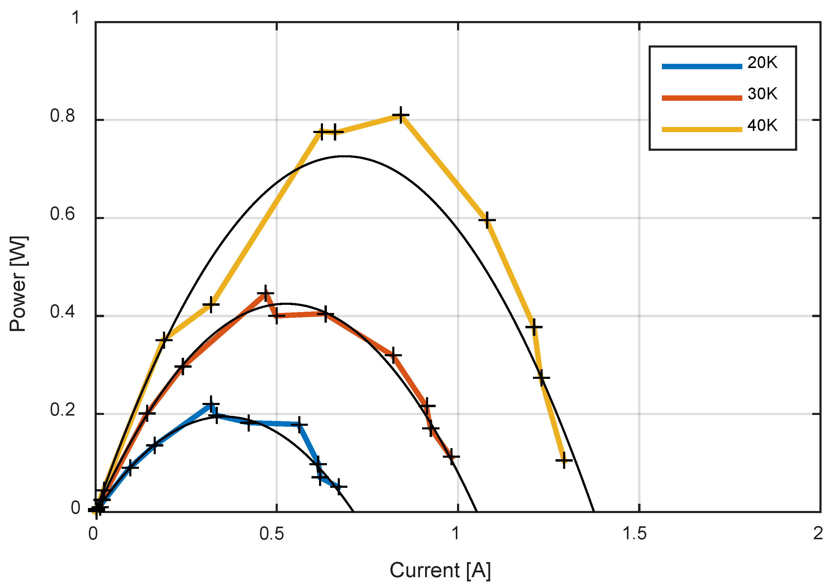
Table 1 compares different TEH approaches using different heat sources, and presents maximum temperature difference and output power.
Using controlled heaters with adjustable temperature permits to evaluate the potential of TEG as energy harvesters, as presented in [10], where a maximum output power of 7.3 W is obtained from a large temperature difference. This type of heat source also provides an estimation of the available power when it is used for environmental sensors. Other sources as ambient light, exterior temperature, and hot asphalt are considered. In [15], a 4-TEG harvester for WSNs is presented. It maintains a temperature gradient of 3 K using ambient temperature as heat source and water as dissipative material. Despite the TEG contains a cold temperature control mechanism, this scheme consists of a DC motor pump that requires an external power source.
Outdoors, solar rays do not achieve higher temperature differences, but arrays can improve the overall output power. In [19], the authors present an autonomous multi-sensor system for agricultural applications using a TEG excited with the incidence of solar rays. The TEG cold side is attached to an aluminum heatsink which allows obtaining a maximum temperature of 8 K and a maximum TEG voltage of 200 mW. In [20], the authors propose a prototype that harvests energy from heat using a thermoelectric material. It consists of an array of 12 TEGs connected in both series and parallel. The TEG hot side is exposed directly to the incidence of solar rays, while the cold side is arranged on water, acting as a dissipative material. In this case, the prototype produces an average temperature gradient greater than 15 K. For both arrays, series and parallel, average powers of 1.23 W and 0.43 W are obtained, respectively.
Such low output powers become a challenge for exploring more efficient mechanisms of energy conversion via TEH. Here, the main goal comes with devising a strategy to increase the temperature difference between the TEG plates/sides to obtain enough energy density to power an IoT sensor. Once the temperature difference is addressed, the soiling effect becomes irrelevant for the TEG option with respect to an SP. Elevating the temperature of one of the TEG plates arises the requirement of maintaining the other plate as close as possible to a reference temperature (i.e., ambient) to maximize the temperature gradient. Active cooling mechanisms decrease the overall efficiency due to the extra power required to operate. As a result, passive mechanisms using heat transfer principles are studied as alternatives to achieve temperature control. Taking advantage of their high specific heat capacity, materials such as water, rock or masonry are used as temperature stabilizers, as seen in Table 1. However, the amount of material required to store energy can be considered high, making them unpractical to size-limited applications. Thus, the use of Phase Change Materials (PCM) can be evaluated. PCMs store and release large amounts of energy compared to sensible heat storage, requiring less mass. For example, in [21], authors perform an experimental study of the thermal performance of a heat pipe with a PCM for electronic cooling. The cooling module with PCM saves 46% of the fan power consumption. In [22], an experimental study is carried in heatsinks with and without PCM to evaluate the best configuration for a high-heat electronic-component generation. The results indicate a maximum temperature reduction of 25% with the insertion of PCMs. Regarding TEGs temperature control, in [23], the authors evaluate the impact of replacing active cooling mechanisms with PCMs to maintain the temperature gradient. Despite the theoretical and simulated results being promising, tests are still developed with water acting as PCM.
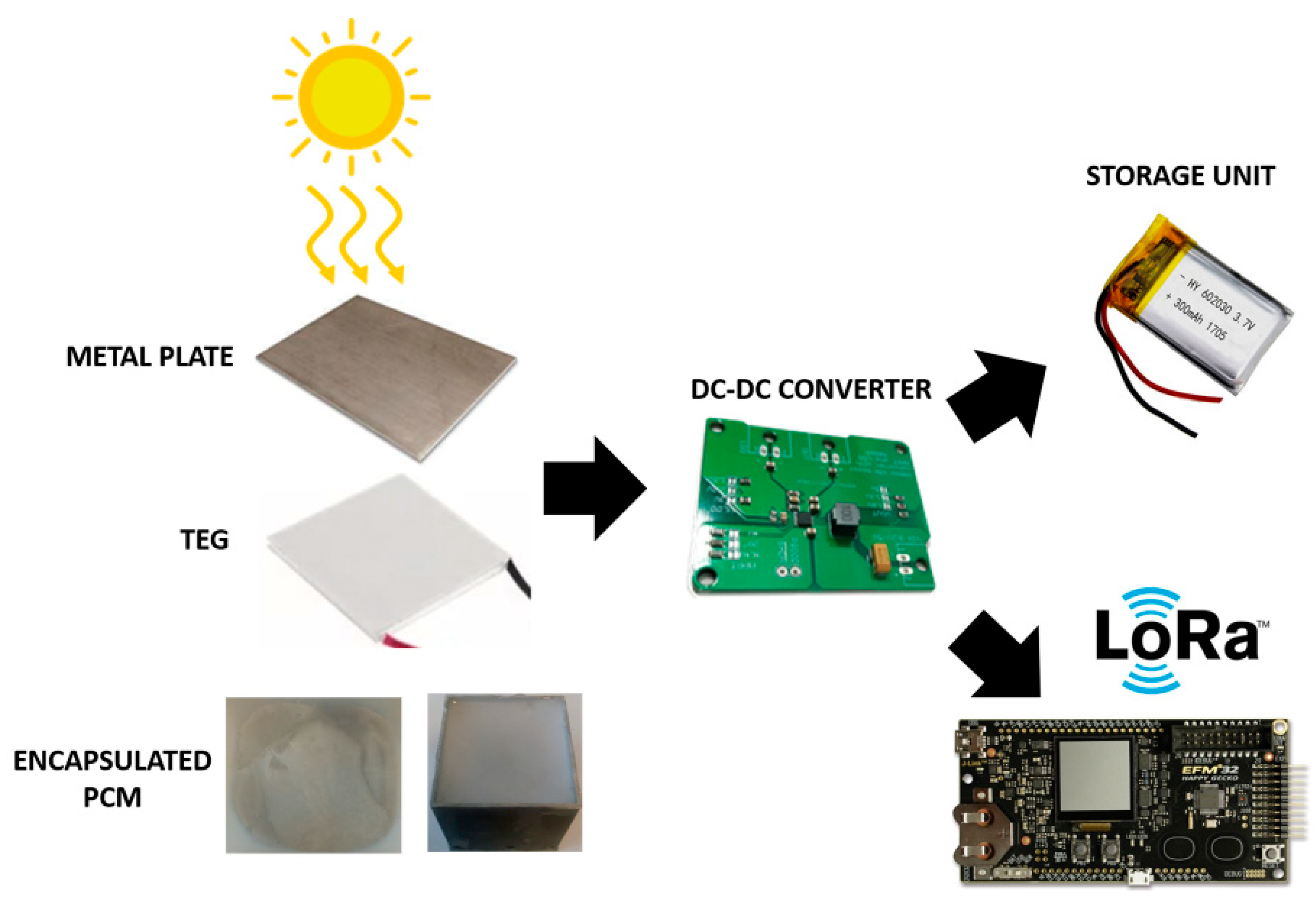
With the presented limitations of TEH for aspects such as output power and dissipative material to maintain the temperature difference, this article proposes an alternative to exploit solar rays as heat source guaranteeing a desired temperature gradient by using PCM as a thermal stabilizer. For this particular development, the solar incident radiation is converted into heat using a metal surface that acts as a concentration element. A commercial PCM is tested as a cooling element to maintain the temperature in the cold plate for proper energy generation. First, a commercial TEG equivalent electrical model is proposed and validated. Then, an energy budget is established to estimate operation time, resulting in a series of specs that allow the development and validation of a complete IoT prototype. Tests of the prototype allow concluding about operation and performance metrics.

2. Materials and Methods

2.1. Thermoelectric Generator

As commented, a TEG converts the temperature differences on its plates/sides into electricity. The TEG is internally composed of a semiconductor material that is doped, producing P-type and N-type legs. These materials are electrically connected in series and thermally connected in parallel, as shown in Figure 1. Electrical energy is produced with the movement of charge carriers from the hot plate to the cold plate via the Seebeck effect [24].
In its simplest form, the TEG can be modeled as a single port element. However, constant parameters such as thermal resistance of the material and the Seebeck coefficient are used to propose the simple electrical equivalent shown in Figure 2.
Assuming that there is no contact resistance between each plate and the legs, the temperatures experienced in the plates (TH and TC) are the same as the ones experienced in the legs ( T H and T C ). As a result, the applied thermal gradient in the plates is equal to the one at P and N legs—that is,
Δ T = T H T C = Δ T = T H T C
The associated DC source is constant and equal to ΔT, so the Open Circuit Voltage (OCV) becomes
V O C = α Δ T
and the output voltage (V) is calculated by applying Kirchhoff’s Voltage Law in the circuit of Figure 2. Thus,
V = α Δ T R E I
Then, the power delivered to a load, RL, becomes
P = α Δ T I R E I 2
Using Equations (3) and (4), the V–I and P–I characteristic curves are constructed and presented on Figure 3. This set of curves is used to determine the corresponding Maximum Power Point (MPP) [25].
With the simplest model presented in Figure 2, MPP can be found from the derivative of Equation (4) as
d P d I = d d I ( V O C I R E I 2 ) = V O C 2 R E I = 0
Then, solving Equation (5) for I
I = I M P P = α Δ T 2 R E
MPP voltage and power are obtained as
V M P P = α Δ T 2
P M P P = ( α Δ T ) 2 4 R E

2.1.1. Characterization

For building a TEH prototype, a commercial thermoelectric module with reference TEC1-12706 and an area of 16 cm2 is selected for characterization. This transducer is chosen given its availability in the limited TEG offering in the local market along with its low price (around USD 2.95). A design of experiments is proposed to validate the TEG electrical model presented in Figure 2. The purpose is to estimate the parameters involved in the transduction process. First, the TEG is tested at several temperature differences and measurements of the OCV, and the temperature gradient are taken to estimate the Seebeck coefficient from Equation (2). The voltage is measured with an Amprobe 37XR-A multimeter. The cold side temperature is measured with a Fluke 80 BK-a K-type thermocouple and the hot side temperature is measured with a Fluke 63 Mini Infrared Thermometer. A metal plate is placed on top of the TEG hot plate and is excited with a heat gun. To maintain the cold plate temperature, a heatsink with a cooling fan is installed. Figure 4 shows the testbench configuration.
The temperature gradient is calculated according to Equation (1). The experiment evaluates temperature differences of 20 K, 30 K, 40 K, and 50 K; and for each temperature difference, 200 measurements are taken. The Seebeck coefficient is therefore empirically calculated using Equation (2) finding an average α of 52.738 mV/K with a standard deviation of 1.976 mV/K. Thus, with confidence intervals of 95%, the true average Seebeck coefficient is estimated between 52.592 mV/K and 52.885 mV/K.
Then, it is necessary to estimate the TEG series resistance. According to Figure 2, the output voltage can be expressed using a voltage divider as
V o = R L R L + R E V O C
Solving Equation (9) for RE, the series resistance is
R E = V O C V o V o R L
Measurements of the output voltage and the temperature gradient are taken for an initial fixed 1 Ω load. This selected value is based on an estimated value of the series resistance provided by the manufacturer according to the semiconductor material of the TEG [26]. The actual series resistance can deviate from the given specification when considering contact resistances between the semiconductor and the ceramic plates. The idea with the 1 Ω-load resistance is to match the theoretical series resistance maximizing the observed output power. Hence, the OCV is calculated with the previously estimated Seebeck coefficient and with measurements of temperature gradients from 10 K to 50 K. Using Equation (10), the average series resistance, RE, is refined to 1.536 Ω with a standard deviation of 0.033 Ω. With confidence intervals of 95%, the true mean series resistance is estimated between 1.534 Ω and 1.538 Ω.
Now, with the estimated Seebeck coefficient and series resistance, it is possible to construct V–I and P–I curves from Equations (3) and (4), as shown in Figure 5 and Figure 6.
In addition to the characteristic curves, it is required to evaluate the voltage and output power of the TEG in the MPP and its variation against temperature differences, that is, V–ΔT and P–ΔT curves. Those are presented in Figure 7.
Hence, with the electrical model and expected behavior, the TEG model is simulated using LTSpice software. First, the mean series resistance and Seebeck coefficient are used as internal parameters. The results of simulated VMPP–ΔT and PMPP–ΔT curves are presented in Figure 8a,b. Then, a Montecarlo simulation is carried out to evaluate the deviation of output voltage and power when internal parameters vary in the confidence intervals. The experiment was repeated 100 times, information is gathered and presented in Figure 8c,d.
Other characteristic parameters such as the figure of Merit (Z-factor) describe TEG behavior. The Z-factor represents the performance of a thermoelectric material through the conversion efficiency. To calculate the Z-factor, parameters as the Seebeck coefficient, thermal conductivity, and resistivity must be considered [27]. During the design process of TEGs, it is an important parameter to maximize because better thermoelectric materials have higher Z-value. However, the figure of Merit is not considered in this prototype because it is based on a commercial module and does not involve the design process of the transducer. Furthermore, for the particular context targeted in this work, it is highly desired to present the performance of outdoor TEH prototype in terms of the main energy source, which is the sun. For that reason the system efficiency is presented and calculated in Section 3.

2.1.2. Operating Conditions

To improve the heat concentration from the solar rays, a metal plate of 16 cm2 is attached to the TEG hot side. Measurements are taken with a Fluke 80 BK-a K-type thermocouple. In a previous work [28], the range of solar radiation hours is classified into ranges according to their statistical characteristics. Times of the day with similar properties are gathered into the same range and average solar radiation is estimated. Table 2 shows the results from a particular design of experiments considering the city of Barranquilla, Colombia, where the final TEG prototype is tested. As observed, an average day can be divided into six ranges, with Ranges V and VI displaying the highest average radiation estimates. Such ranges are the targeted operation hours for TEH.
Initially, temperature measurements are taken every five minutes from 9 a.m. to 3 p.m. for five days in the selected ranges. Then, it is found that the average temperature is 334.017 K (60.87 °C), with a standard deviation of 1.13256 K. Measurements presented in Figure 9 show that the temperature increases during the selected ranges as the metal plate is excited by the sun rays. It is important to note that the hot plate temperature does not require any type of mirror and/or magnifying glass.
For the cold plate, it is required to set a temperature up to 302 K (28.85 °C) given the measurements displayed in Figure 9; so that, the TEG output power can provide a TEG efficiency higher than 20%. The 20% efficiency lower limit is selected because it corresponds to high-end SP efficiencies. The authors’ goal is to show that the TEG minimum efficiency is at least as good as high-quality SPs. The challenge is that given the natural conduction between the TEG hot and cold plates, there exists the tendency of the cold-plate temperature to increase if not well regulated; which in turn decreases the temperature difference and, therefore, the power delivered by the module.
Thus, it is necessary to establish a mechanism to keep ΔT at the expected values maintaining the expected available power. Even though cooling fans or other active strategies can be used, the power drawn from the TEG makes this approach not energetically appealing for IoT applications. Thus, a particular dissipative material must be attached to regulate the cold plate at the required temperature, but the advantage in this work is that such temperature regulation is obtained by passive means.
In a previous work [28], the use of wet particles as a dissipative material was evaluated with satisfactory results; however, the continuous watering of the particles makes the approach somewhat impractical. In any case, the results obtained lead to explore other materials such as the Phase Changing Materials (PCMs) that can maintain the cold side temperature, as described in Section 3.2.

2.1.3. Model Validation

Thus, defining the operating conditions described in the previous section, a model validation via simulation is proposed for the expected temperature gradient of 30 K. To that end, the electrical model is constructed in LTspice with the refined parameters. The V–I and P–I curves are constructed and shown in Figure 10. Table 3 summarizes the simulated MPP conditions.
Then, a Montecarlo simulation is performed to evidence the changes that would occur in the output power due to the variation in the internal parameters and operating conditions during the day based on the confidence intervals calculated previously. The MPP and voltage at MPP are evaluated. It is found that the MPP is 428.011 mW with a standard deviation of 41.992 mW. Thus, for the authors claim of minimum efficiency of 20%—given the TEG area and the average radiation for Ranges V and VI (see Table 2)—for the worst case, the average output power is 386.019 mW, resulting in an efficiency of 28.73% (for 20% efficiency the output power would have to be 268.87 mW). Furthermore, as an input spec for the later IoT-sensor power-management-unit design, the average MPP voltage is 408.036 mV with a standard deviation of 20.83 mV (the average MPP voltage is between 407.8 mV and 408.27 mV with 95% of confidence).

2.2. Phase Change Material

2.2.1. Material Description

PCMs are substances that storage latent heat of fusion. They exchange a large amount of heat through a change in their physical state [29]. The thermal energy transfer occurs during the solid-liquid or liquid-solid phase changes. Unlike sensible storage materials, PCM storage systems have the advantage that they operate with small temperature differences during the phase change while store or release thermal energy. They can store 5–14 times more energy per unit of volume than sensible storage materials such as water, masonry, or rock [30]. Heat storage profiles based on temperature for single-phase and PCM materials are presented in Figure 11.
Some applications of PCM as latent heat units are found in solar water heaters, where sensible heat in a fluid is increased to achieve thermal energy storage [32]. Replacing the fluids with a PCM reduces the amount of volume due to the use of sensible heat. The solid-liquid transformation permits the system to store energy during the day and release energy during the night [33]. For this work, the PCM fulfills the function of thermal stabilizer. A commercial paraffin wax is used as the PCM with a melting point range of 302.15 K (29 °C)–308.15 K (35 °C), and other properties summarized in Table 4 [34].
Among the issues faced when using this material as a thermal stabilizer is the volume expansion during its phase change. The volume increases by approximately 10% from solid to liquid. As the PCM is located below the TEG, there is a possibility that the PCM does not adhere to the TEG cold plate because of the gravity effect, reducing the effectiveness of the intended passive cooling mechanism. Consequently, the PCM is encapsulated in a metal cube with a volume of 64 cm3. Thus, a total amount of 0.055 kg of PCM is placed inside the cubic container that later is placed under TEG as presented in Figure 12.

2.2.2. Operating Conditions

Using a testbench with the metal plate on the TEG hot side, and the PCM on the cold side, the TEG is tested at the incidence of solar rays to estimate the actual temperature gradient range. For the sake of comparison, measurements replacing the PCM with a metal heatsink are also recorded every three minutes. The two devices-under-test are shown in Figure 13.
Measurements are taken for two days allowing to estimate the actual temperature gradient experienced by both TEG arrangements with a total of 720 samples. With the set of measurements for both cases, it is possible to analyze the temperature-gradient behavior with both average solar radiations below and over as extreme cases (see Table 2). The results are summarized in Figure 14. As observed, the temperature gradient at the end of the day is higher for the PCM case in both experiments, which indicates that the system has been thermally regulated with a passive scheme.
It is important to note that in situations with radiation over the average, when it is expected to harvest the most energy, the testbench with the heatsink is unable to maintain the temperature gradient as heat transfers from the hot plate to the cold side reducing the electrical output power accordingly. The prototype with heatsink could only be used with solar radiation below the average which is clearly inefficient. To calculate the expected energy, the area under the output power curve is approximated using the trapezoid method.
Furthermore, in the design of experiments, the expected energy is evaluated in Ranges V and VI with samples every five minutes. Thus, during the six-hour time-frame, the expected average power and energy are calculated based on temperature gradient measurements. The results are listed in Table 5.

2.3. Prototype Description

Once the TEG is modeled and validated, and the passively-regulated thermal strategy is demonstrated experimentally, a fully functional outdoor IoT sensor prototype is devised. The IoT sensor block diagram is presented in Figure 15. It consists of one TEG (with the metal plate and the PCM), a low-power microcontroller with a temperature/humidity sensor, a low-power radio transceiver, a DC-DC converter, and a 3.7 V 550 mAh Li-Po battery as a storage unit. Given that the TEG approach has been discussed previously, the complementing blocks are described next.

2.3.1. Microcontroller, Environmental Sensor and Radio Transceiver

As commented, an IoT application requires a low-power microcontroller. Thus, an EFM32 Happy Gecko Evaluation Board (from Silicon Labs, Austin, TX, USA) is selected for that purpose. The EFM32 is a 3.3 V ultra-low power and easy-to-deploy device that demands a power consumption in both active and sleep modes of 528 μW and 1.98 μW, respectively. It contains an on-chip SI7021 environmental sensor that measures from 233 K (−40.15 °C) to 358 K (84.85 °C) temperature and 0% to 80% relative humidity. An RN2483 LoRa transmitter is used as a radio transceiver. Using the parameters reported by the manufacturers, an initial theoretical energy budget is estimated and summarized in Table 6. Under this approach, it is proposed to carry out the environmental variable measurements and sending the data info every 30 min. The budget contemplates data reading, processing, sending, and microcontroller shut-off mode. Thus, a total energy of 1032.643 mWh is needed by the IoT sensor during the 24 h. In Ranges V and VI, the TEH must be able to power up the system with 258.161 mWh and store the remaining energy. Therefore, outside the preferred solar ranges, a storage system must provide 774.482 mWh for continuous operation. Table 6 shows that the required peak power is not superior to the peak power that the TEH can provide.

2.3.2. Power Management Unit

An adequate power management unit becomes crucial for proper sensor operation. As the total equivalent load changes, the supply system must be capable of providing a sufficient amount of power. DC-DC converters are circuits that convert a DC voltage to a different DC regulated level with high efficiency (>80%). The DC-DC converters can increase or reduce the output voltage compared to the input voltage according to the application, and some are also designed to find the MPP [35]. Some approaches that perform MPP searching include Maximum Power Point Tracking (MPPT) techniques, including Perturbate and Observe (P&O), Incremental Conductance (IC), Parasitic Capacitance (PC), and Open Circuit Voltage (OCV) [36,37]. The OCV method assumes that the operating voltage at the MPP does not vary significantly. It is used for TEGs considering the low change percentage in the MPP [38].
Given the TEH available power, a DC-DC converter is included to manage the circuitry and on-board battery. An LTC-3105 development board from Linear Technology (Analog Devices) is selected for this purpose since it is typically used for Solar EH and TEH applications. The circuit is designed to operate using the OCV method for MPPT. Using the parameters recommended by the manufacturer [39], a resistor divider is connected between the Vout and FB pins to program the step-up converter output voltage as
V O U T = 1.004 ( R 1 R 2 + 1 )
which allows setting the output voltage to 3.7 V. Thus, it is possible to handle not only the battery but also the microcontroller, which would permit to use a single supply voltage ranging from 1.98 V to 3.8 V. This is, in part, due to an embedded 3.3 V regulator in the development board for the on-chip sensors and for the supply of power to the radio transceiver. Furthermore, according to the manufacturer, the LTC3105 has been optimized for use in power sources as TEG and SPs by presenting an output resistance of 0.5 Ω.
According to Equation (9), the MPP voltage is considered half the OCV [40]. Furthermore, considering the TEG Montecarlo simulation, it has been validated that with the selected temperature gradient, the MPP voltage changes around 0.11%. As a result, there is no need to implement an MPPT algorithm, but to use and fix with the TEG average MPP voltage. Thus, with the information of Table 3 about MPP conditions and current suggested by the manufacturer, the MPPT resistor is calculated as
R M P P T = V M P P 10 μ A
Figure 14 presents the SPICE testbench for the validated TEG source, DC-DC converter and a variable load resistor. The proper operation of the DC-DC converter is evaluated with load resistances ranging from 50 Ω to 1.5 kΩ. It is found that the converter delivers a maximum output power of 420.38 mW.
Therefore, the efficiency of the DC-DC converter can be calculated as
η = P O U T P T E G × 100 %
Using statistical validation from the simulated results obtained for the range of load resistors, the average efficiency is found to be 81.8276% with a standard deviation of 2.98%. The efficiency mean is between 80.1773% and 83.4779% with 95% confidence. Given an 80% worst-case efficiency, the energy budget can be adjusted to account for the losses associated with the DC-DC converter. Thus, the new total energy becomes about 1290.8 mWh for a complete day, a supply of 322.7 mWh from the TEH during Ranges V and VI, and the additional 968.1 mWh for the other operation ranges to guarantee continuous operation.

2.3.3. Storage Unit based on a Li-Po Battery

Storage units can be employed to complement the operation of TEH when the main source (solar radiation) is not available, such as nighttime. To properly size the required storage unit; first, the expected average power and energy must be considered (see Table 5). Then, with the validated internal parameters and the measured temperature gradient from Section 3.2, the MPP is calculated using Equation (8). Considering the estimated power consumption for the microcontroller, environmental sensor, and radio transceiver, secondary batteries and supercapacitors are evaluated as options. Secondary battery energy densities are one or two orders of magnitude higher than supercapacitors but present higher series resistance. Thus, considering initially a capacitor, the stored energy is defined as
W = 1 2 C V 2
then, to maintain a discharge percentage of 50% and to provide the required energy outside Ranges V and VI, the supercapacitor capacity should be twice the required capacity, that is 1936.2 Wh (6970.32 J). Since supercapacitor voltages usually vary from 2.2 V to 3.3 V, then using the maximum voltage, a capacitance of 1280.1 F would be required. As a result, a supercapacitor is not a practical option as a storage unit given the energy capacity requirements for the IoT sensor.
Therefore, among secondary batteries, lithium-based batteries are most widely used for portable and space-constrained devices. These batteries present capacities less than 1 Ah and operate up to 20 years over a wide temperature range. Thus, for the required 1936.2 Wh (outside Ranges V and VI) a 3.7 V 550 mAh Li-Po battery meets the required energy specification. It is important to note that a 50% depth-of-discharge (DoD) is initially considered to have a proper trade-off between cost and lifetime. Since the battery capacity is 2035 Wh, a first-order approximation indicates that the IoT sensor is operating with a 53.41% DoD, which indicates that the battery lifetime is slightly improved.

2.3.4. Simulation of TEH Prototype

After completing the design of the TEH scheme, it is simulated in LTSpice software using the schematic presented in Figure 16. The average Seebeck coefficient and series resistance are used as internal parameters for the TEG. Temperature difference measurements of Figure 14 establish the simulation input variables to evaluate expected output power and voltage based on the electrical models of the components and previous measurements. Figure 17 shows the simulation of the TEH prototype at a minimum temperature difference of 27.8 K, and Figure 18 at a maximum temperature difference of 34.5 K.
The expected average input power varies from 375 mW to 565 mW, while the expected average output power at the load (battery and sensor) varies from 328 mW to 517 mW. If the efficiency of the DC-DC converter is defined as
η = P O U T P I N × 100 %
Then, from the simulations, the efficiency for the DC-DC converter results in a variation from 87.46% to 91.5%. This agrees with the parameters presented in the converter specs.

3. Experimental Results

3.1. Characteristic Curves of TEG

The construction of characteristic curves with measurements is fundamental to finish the validation of the presented electrical model for TEGs and analyze expected power and energy. Using the testbench presented in Figure 4, the TEG behavior is tested with three different temperature differences and compared with data presented in Figure 5 and Figure 6. The TEG is excited with the heat gun to achieve theoretical temperature gradients of 20 K, 30 K and 40 K, considering that the prototype is expected to work around 30 K. Measurements of voltage, power, and current are taken with the multimeter, while a mini infrared thermometer is added to measure both plates temperature at the same time. Table 7 presents the average and standard deviation for the selected temperature differences.
Twelve resistances are used as load resistances, varying from 0.12 Ω to 1 kΩ. From the Maximum Power Transfer Theorem, the MPP of every linear circuit is obtained when the load resistance equals the internal resistance. Since TEG load resistance is found to be 1.536 Ω, the TEG is tested with low resistances. Since a precision potentiometer is not sensible enough for such low resistances, they are obtained with series-parallel arranges of commercial resistors. The results of the V–I and P–I curves are presented in Figure 19 and Figure 20.
The theoretical curves are compared with the obtained measurements using average temperature differences presented in Table 7. A maximum variation of 0.13 V is observed in V–I curve, while a maximum variation of 107 mW is presented in P–I curve, for ΔT = 40 K. For the expected operating conditions (30 K), the measurements validate the electrical model presented in Section 3.1 and the simulation of Figure 8.
As V–I and P–I curves are compared with theoretical equations, it is also mandatory to measure V–ΔT and P–ΔT, and compare them with expected behavior in simulations of Figure 8. With the same testbench, a 1.51 Ω resistance is connected as a load of the TEG to equal the internal resistance. The heat gun excites the TEG to get temperature difference measurements from 0 to 60 K, with steps of 5 K. Furthermore, voltage and power measurements are taken. Figure 21 shows the comparison between the ideal and experimental curves.
Temperature difference measurements vary from ideal steps. However, curve trends are maintained, with a maximum difference of 0.124 V for voltage curve and 92 mW for MPP curve. As a result, the model that relates the dependence of the TEG voltage and power with respect to temperature is validated.

3.2. Performance Tests of TEH Prototype

Figure 22 shows the encapsulated prototype based on the components listed and dimensioned previously. The information sent by the prototype is received by a LoraWan gateway installed on Universidad del Norte campus. All the information that is sent to this gateway is displayed in a custom-made user interface. Figure 22 also shows the measurements taken with the mentioned sensors and the GPS position referencing the position of Universidad del Norte. With the device, a design of experiments is carried out to evaluate its performance according to the estimated energy budget considered.
First, measurements of radiation are obtained from available data of a local Davis Vantage Pro 2 Personal Weather Station (PWS). The PWS reports weather variables every 15 min; thus, solar radiation measurements for 60 days (during March, April and May 2019) for Ranges V and VI are gathered. For that particular set of information, the percentiles for the average solar radiation are calculated and summarized in Table 8. Assuming a normal distribution, both tails of 10% are used to determine that 5.0% of the mean radiation is below 383.0 W/m2 and 5% of the mean radiation is over 907.357 W/m2.
Then, the devised IoT sensor is placed under the influence of solar rays with the battery completely discharged. Measurements of TEG output current, voltage and MPP voltage are used to obtain the input power of the TEH scheme. The results are presented in Figure 23.
As noticed, TEG output voltage increases during the day according to the temperature gradient, while the DC-DC converter MPP voltage presents minimum variations around the selected power-point. When the TEG voltage is below 1.6 V, the DC-DC converter output is lower than the OCV. However, it provides the current required for the battery and load. The measurements in Figure 23 permit the estimation of an input resistance for the TEH prototype. Using Equation (9) and all data points for the TEG MPP and TEG currents, a mean input resistance of 1.618 Ω with a standard deviation of 0.012 Ω is calculated. Moreover, ripple voltage can be obtained from the TEG MPP voltage curve. The mean voltage and maximum deviations are calculated for each day for a ripple voltage varying between ±0.043 V to ±0.125 V.
Figure 24 and Figure 25 show the power delivered by the prototype in Ranges V and VI for the corresponding days laying on percentiles 5% (three days) and 95% (two days).
To establish a comparison with powering units that use the sun as energy source, the TEG efficiency is calculated from equation for solar panels as
η = M P P r a d i a t i o n × a r e a
Notice that the TEG area equals 16 cm2; then, given the average solar radiation value for the Range VI (see Table 8), the maximum output power potential would for a η = 100% would be 1.34 W. However, considering the η = 20% target for good quality solar panels, the expected power output from the TEH should be at least 268 mW. Using the measurements presented in Figure 24, an average output power variation from 335 mW to 480 mW is obtained with a mean efficiency of 26.43%. This span produces an average efficiency that ranges from 21% to 34.38%. The efficiency is calculated using Equation 16 and the incident radiation for each particular day. In any case, a statistical validation is carried out to determine if the complete prototype maintains the claimed efficiency (over 20%) during the selected ranges; that is, the average output power is greater than 320 mW. Considering the proposed hypothesis test, the one-tail model of the standard normal distribution is used to reject the null hypothesis. The left tail of the distribution is taken for a level of significance of α equal to 5% and with it, a Z = −1.645. The Z statistic for this type of test is greater than the 0.05 Z-value considered according to the level of significance. Therefore, the null hypothesis is rejected with a 95% certainty. This means that the average output power is greater than 320 mW and the efficiency is maintained over 20% with 95% confidence.
Table 9 presents the total energy produced in both types of radiation levels considered. As observed, about 2 Wh is harvested from the TEG for the worst-case scenario, and from the energy budget consideration of Section 3.2, the TEH scheme provides enough energy—not only to power up the microcontroller, sensors, and radio transceiver, but also to charge the battery during the selected ranges. Finally, a maximum power of 132 mW is required when the transceiver is sending, and since the TEG average power surpasses that value, the harvester is also capable of maintaining the transceiver powered.
Outside the selected ranges with no current flowing to the battery, a maximum load of 61.6 mW can be connected to the system maintaining a discharging percentage of 50% of the battery. The battery satisfies the energy demand in a maximum time of 18 h without charging. The microcontroller, sensor, and transceiver consume 49.91% of the energy produced by the TEG. The remaining energy can be stored for the operation outside the selected ranges. The battery was connected fully discharged and was charged during the selected ranges by the prototype. With these estimates, the TEH prototype is tested for two days to verify the operation during the entire day. Solar radiation is measured with the PWS and the reports of temperature and humidity are taken from the data sent by the unit. The results are presented in Figure 26.
The system presented a blackout between whether 5 a.m. and 7 p.m. According to Table 9, an average DoD of 38.058% of the battery capacity is expected. However, on the first day, solar radiation measurements were not the expected values. With the battery completely discharged, the harvested energy was not enough to maintain the operation during the night. On the other hand, solar radiation was high on Day 2, causing the battery to be charged and ready to operate the entire night.

4. Conclusions

This paper has shown a complete energy harvesting system with passive cooling that supports the operation of a secondary battery to power up outdoor sensors. The energy harvesting strategy employs the solar resource but increases the conversion efficiency, reducing adverse effects such as heating and soiling exhibited by solar panels. Thus, the thermal gradient is preferred over the photovoltaic effect. The complete harvesting system complements the TEG selected as a transducer with all the required blocks to properly manage battery cycles that maximize lifetime by ensuring a DoD lower than 50%.
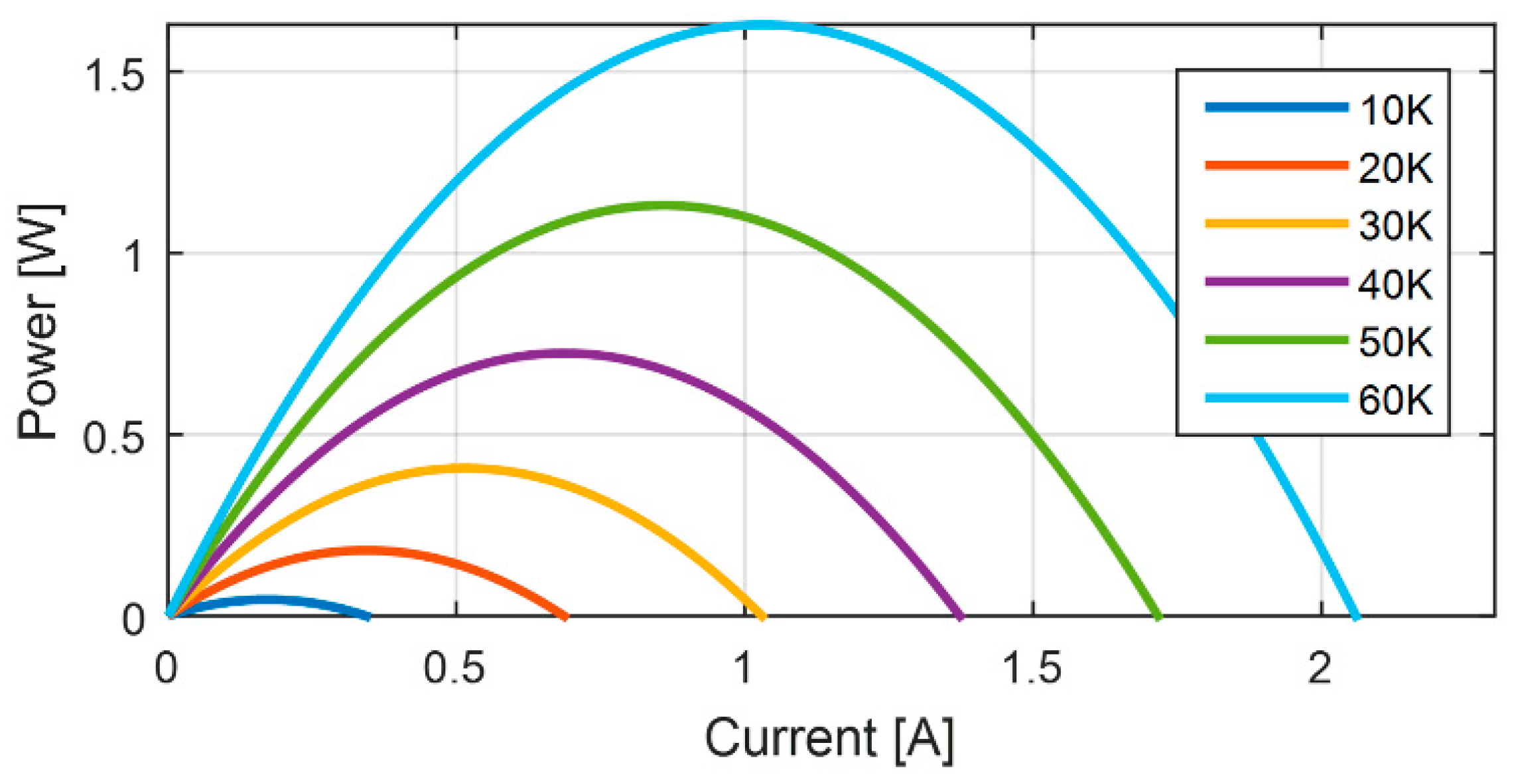
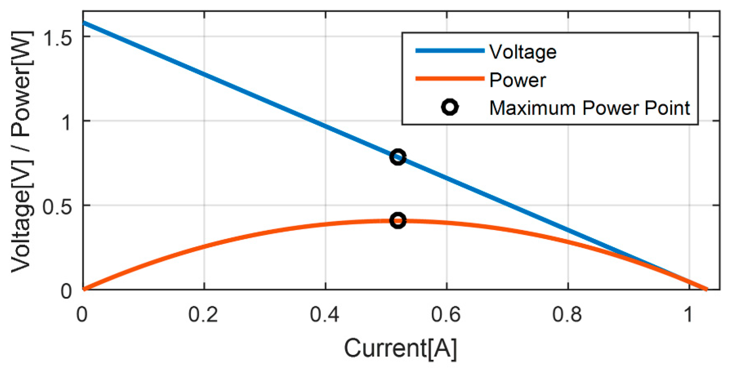
Characterizing a TEG is important to determine the associated electric potential and for simulation purposes. Initially, a first-order transducer model has been proposed based on the associated basic electrical parameters. It is shown that 407.3 mW output power and 2.4438 Wh energy are obtained using SPICE-based simulations helping the design process.
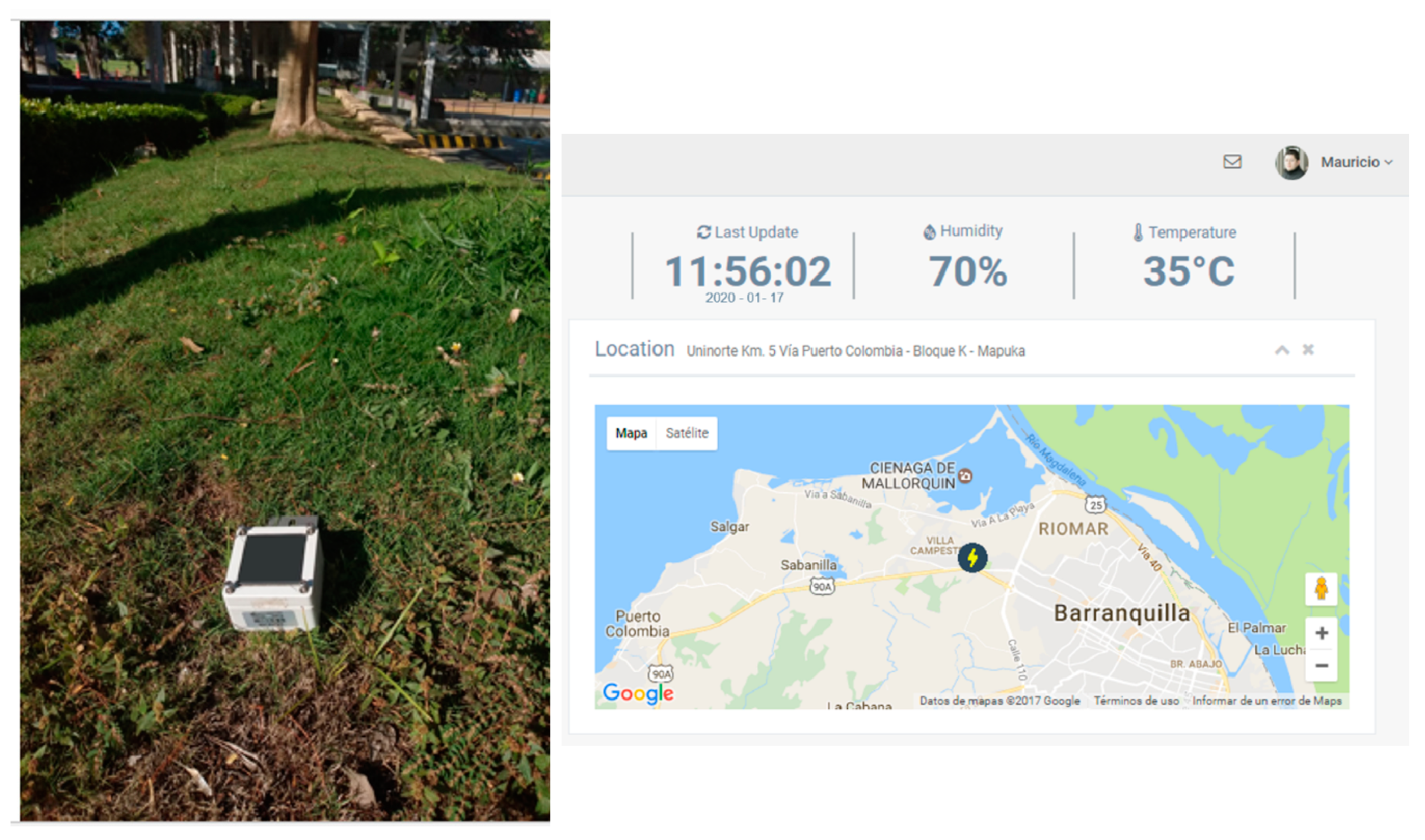
The key aspect for proper use of thermoelectric harvesting is maximizing the temperature gradient that experiences a TEG given certain environmental conditions. For the case of this work, the City of Barranquilla counts with ample solar resource; therefore, a metal plate is attached to the TEG hot-plate for proper thermal conduction, and a dissipative material is required to keep the initial TEG cold-side temperature. The PCM becomes the ideal choice as dissipative material when selected so that the material changes its phase at a temperature as close as possible to the ambient temperature. Thus, while the metal plate continues to heat up, the cold side temperature is maintained, keeping the targeted temperature gradient and with that the desired efficiency.
To verify its advantage for cooling, the PCM is compared to a heatsink. It is found that the PCM reaches an average temperature gradient of 33.1 K, while the heatsink only gets an average temperature gradient of 31.05 K. This represents an improvement of 2.05 K, which corresponds to an average of 106 mW more power. For the selected operating hours this produces about 424 mWh more or a gain of 14.37% in the total harvested energy.
In this work, a complete outdoor IoT sensor is built as a testbench to demonstrate proper energy supply from a TEH. The prototype contains a low-power microcontroller and environmental sensors that measure ambient temperature and relative humidity, and is equipped with a low-power radio to report the variables to a central node/gateway. It is found that employing the TEG with the passive cooling strategy, the TEH has enough power to operate the microcontroller, sensors, and radio, that demand average energy of 1.032 Wh during the day. Furthermore, it is demonstrated that the prototype supplies sufficient energy for continuous operation even during times with no solar resource through an on-board 2.035 Wh battery. Such a battery can be recharged once the solar radiation is available without compromising sensor operation.
Corroborating that there is enough energy for sensor autonomy is determined mainly in the case of days with solar radiation below the estimated average for the geographical zone considered. Thus, the designers are considering the worst-case scenario.
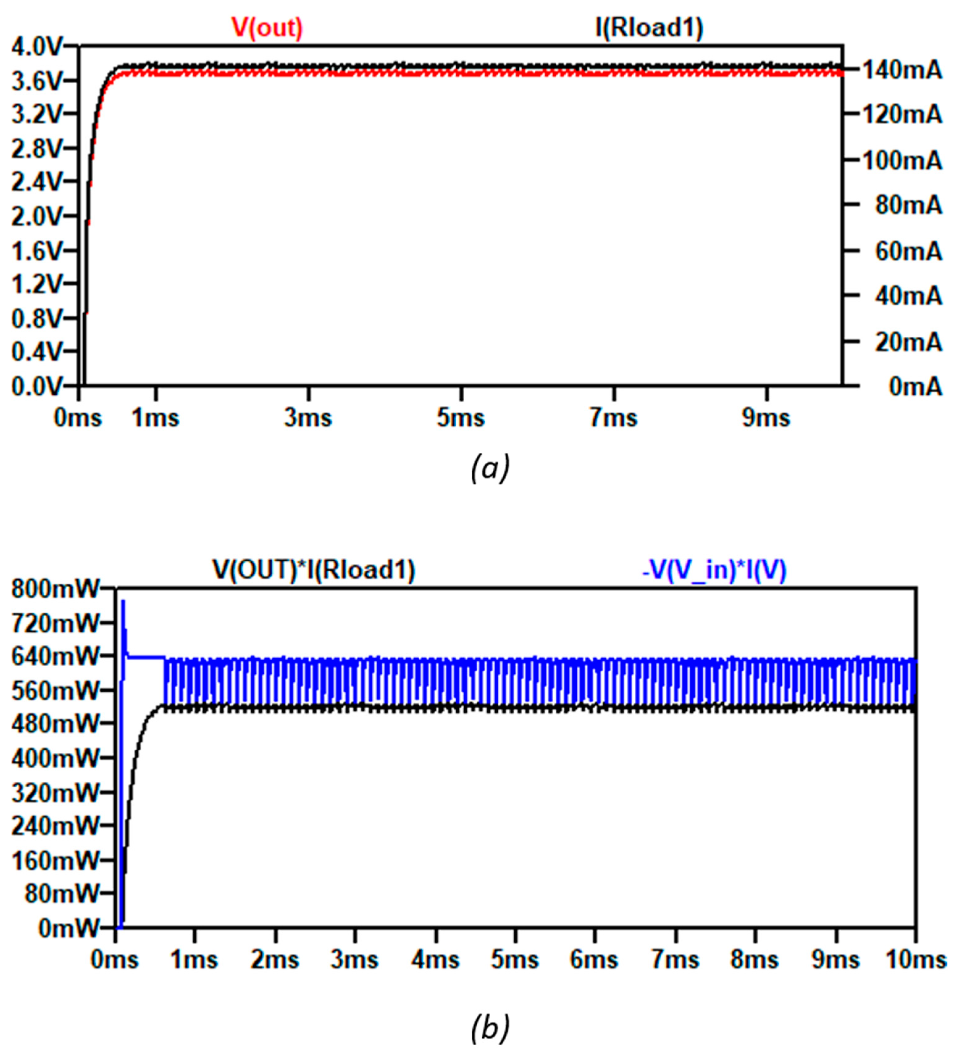
Power electronics have proved their contribution to adequate power into the proper voltage and current ranges defined by the sensor circuitry. An 80.81% average efficiency DC-DC converter is selected as a power management unit.
Last, the authors have been able to demonstrate the efficiency claim of solar radiation conversion over SP efficiencies. Statistically, it is found that the efficiency of the prototype surpasses 20% with 95% confidence in solar-radiation Ranges V and VI. Furthermore, the TEH strategy does not suffer from efficiency reductions due to solar panel heating and/or soiling. It has been shown that with a TEH area of only 16 cm2, a minimum of 2.45 Wh can be easily harvested over a six-hour time span, and such an energy level is enough for low-power oriented sensors.

Author Contributions

Conceptualization, D.C., A.R.O., M.C. and M.P.; Data curation, D.C. and A.R.O.; Formal analysis, D.G., M.C. and M.P.; Funding acquisition, D.G.; Investigation, D.C., D.G., A.R.O., and M.P.; Methodology, D.C., D.G., A.R.O., M.C. and M.P.; Resources, D.G.; Supervision, M.P.; Validation, D.C., M.C. and M.P.; Visualization, D.G.; Writing—original draft, D.C., A.R.O. and M.P.; Writing—review and editing, D.C., D.G., M.C. and M.P. All authors have read and agreed to the published version of the manuscript.

Funding

This research was funded by the National Fund for Financing Science, Technology and Innovation—Francisco José de Caldas Fund—of the Colombian government, through the call for registration of projects that aspire to obtain tax benefits for investment in science, technology and innovation (call 741 of 2016).

Conflicts of Interest

The authors declare no conflict of interest.

References

  1. Ismagilova, E.; Hughes, L.; Dwivedi, Y.K.; Raman, K.R. Smart cities: Advances in research—An information systems perspective. Int. J. Inf. Manag. 2019, 47, 88–100. [Google Scholar] [CrossRef]
  2. Dehghani-Sanij, A.R.; Tharumalingam, E.; Dusseault, M.B.; Fraser, R. Study of energy storage systems and environmental challenges of batteries. Renew. Sustain. Energy Rev. 2019, 104, 192–208. [Google Scholar] [CrossRef]
  3. Kousksou, T.; Bruel, P.; Jamil, A.; El Rhafiki, T.; Zeraouli, Y. Energy storage: Applications and challenges. Sol. Energy Mater. Sol. Cells 2014, 120, 59–80. [Google Scholar] [CrossRef]
  4. Penella-López, M.T.; Gasulla, M. Ambient Energy Sources. In Powering Autonomous Sensors: An Intergral Approach with Focus on Solar and RF Energy Harvesting; Springer: Dordrecht, The Netherlands, 2011; pp. 29–38. [Google Scholar] [CrossRef] [Green Version]
  5. Green, M.A.; Hishikawa, Y.; Dunlop, E.D.; Levi, D.H.; Hohl-Ebinger, J.; Yoshita, M.; Ho-Baille, A.W.Y. Solar cell efficiency tables (Version 53). Prog. Photovolt. Res. Appl. 2019, 27, 3–12. [Google Scholar] [CrossRef] [Green Version]
  6. Zhang, J.; Xuan, Y. An integrated design of the photovoltaic-thermoelectric hybrid system. Sol. Energy 2019, 177, 293–298. [Google Scholar] [CrossRef]
  7. Ando Junior, O.H.; Maran, A.L.O.; Henao, N.C. A review of the development and applications of thermoelectric microgenerators for energy harvesting. Renew. Sustain. Energy Rev. 2018, 91, 376–393. [Google Scholar] [CrossRef]
  8. Alghoul, M.A.; Shahahmadi, S.A.; Yeganeh, B.; Asim, N.; Elbreki, A.M.; Sopian, K.; Tiong, S.K.; Amin, N. A review of thermoelectric power generation systems: Roles of existing test rigs/ prototypes and their associated cooling units on output performance. Energy Convers. Manag. 2018, 174, 138–156. [Google Scholar] [CrossRef]
  9. Hou, L.; Tan, S. A preliminary study of thermal energy harvesting for industrial wireless sensor networks. In Proceedings of the 2016 10th International Conference on Sensing Technology (ICST), Nanjing, China, 11–13 November 2016; pp. 1–5. [Google Scholar] [CrossRef]
  10. Guan, M.; Wang, K.; Xu, D.; Liao, W.H. Design and experimental investigation of a low-voltage thermoelectric energy harvesting system for wireless sensor nodes. Energy Convers. 2017, 138, 30–37. [Google Scholar] [CrossRef]
  11. Zaman, H.U.; Shourov, C.E.; Al Mahmood, A.; Siddique, N.E.A. Conversion of wasted heat energy into electrical energy using TEG. In Proceedings of the 2017 IEEE 7th Annual Computing and Communication Workshop and Conference (CCWC), Las Vegas, NV, USA, 9–11 January 2017; pp. 1–5. [Google Scholar] [CrossRef]
  12. Lebahn, F.; Ewald, H. Using atmospheric temperature variations for thermal energy harvesting for wireless sensors. In Proceedings of the 2015 9th International Conference on Sensing Technology (ICST), Auckland, New Zealand, 8–10 December 2015; pp. 133–137. [Google Scholar] [CrossRef]
  13. Prijic, A.; Vracar, L.; Vuckovic, D.; Milic, D.; Prijic, Z. Thermal energy harvesting wireless sensor node in aluminum core PCB technology. IEEE Sens. J. 2015, 15, 337–345. [Google Scholar] [CrossRef]
  14. Yun, M.; Ustun, E.; Nadeau, P.; Chandrakasan, A. Thermal energy harvesting for self-powered smart home sensors. In Proceedings of the 2016 IEEE MIT Undergraduate Research Technology Conference (URTC), Cambridge, MA, USA, 4–6 November 2016; pp. 1–4. [Google Scholar] [CrossRef] [Green Version]
  15. Verma, G.; Sharma, V. A Novel Thermoelectric Energy Harvester for Wireless Sensor Network Application. IEEE Trans. Ind. Electron. 2019, 66, 3530–3538. [Google Scholar] [CrossRef]
  16. Tahami, S.A.; Gholikhani, M.; Nasouri, R.; Dessouky, S.; Papagiannakis, A.T. Developing a new thermoelectric approach for energy harvesting from asphalt pavements. Appl. Energy 2019, 238, 786–795. [Google Scholar] [CrossRef]
  17. Jiang, W.; Yuan, D.; Xu, S.; Hu, H.; Xiao, J.; Sha, A.; Huang, Y. Energy harvesting from asphalt pavement using thermoelectric technology. Appl. Energy 2017, 205, 941–950. [Google Scholar] [CrossRef]
  18. Singh, M.; Singh, J.; Anshula; Kuchroo, P.; Bhatia, H.; Bhagat, S.; Sharma, G.; Sidhu, E. Efficient autonomous solar panel and thermo-electric generator (TEG) integrated hybrid energy harvesting system. In Proceedings of the 2016 Progress in Electromagnetic Research Symposium (PIERS), Shanghai, China, 8–11 August 2016; pp. 1764–1768. [Google Scholar] [CrossRef]
  19. Dias, P.C.; Morais, F.J.O.; de Morais França, M.B.; Ferreira, E.C.; Cabot, A.; Siqueira Dias, J.A. Autonomous Multisensor System Powered by a Solar Thermoelectric Energy Harvester With Ultralow-Power Management Circuit. IEEE Trans. Instrum. Meas. 2019, 64, 2918–2925. [Google Scholar] [CrossRef]
  20. Singh, J.; Kuchroo, P.; Bhatia, H.; Sidhu, E. Floating TEG based solar energy harvesting system. In Proceedings of the 2016 International Conference on Automatic Control and Dynamic Optimization Techniques (ICACDOT), Pune, India, 9–10 September 2016; pp. 763–766. [Google Scholar] [CrossRef]
  21. Weng, Y.; Cho, H.; Chang, C.; Chen, S. Heat pipe with PCM for electronic cooling. Appl. Energy 2011, 88, 1825–1833. [Google Scholar] [CrossRef]
  22. Ali, H.M.; Saieed, A.; Pao, W.; Ali, M. Copper foam/PCMs based heat sinks: An experimental study for electronic cooling systems. Int. J. Heat Mass Transf. 2018, 127, 381–393. [Google Scholar] [CrossRef]
  23. Kiziroglou, M.E.; Wright, S.W.; Toh, T.T.; Mitcheson, P.D.; Becker, T.; Yeatman, E.M. Design and Fabrication of Heat Storage Thermoelectric Harvesting Devices. IEEE Trans. Ind. Electron. 2014, 61, 302–309. [Google Scholar] [CrossRef]
  24. Zhang, X.; Zhao, L.D. Thermoelectric materials: Energy conversion between heat and electricity. J. Mater. 2015, 1, 92–105. [Google Scholar] [CrossRef] [Green Version]
  25. Paraskevas, A.; Koutroulis, E. A simple maximum power point tracker for thermoelectric generators. Energy Convers. Manag. 2016, 108, 355–365. [Google Scholar] [CrossRef]
  26. Thermonamic Electronics. Specification of Thermoelectric Module TEC1-12706. Available online: http://www.thermonamic.com/TEC1-12706-English.PDF (accessed on 31 March 2020).
  27. Hossain, M.M.; Ahmed, S.A.; Shahriar, S.M.; Zzaman, M.S.; Das, A.; Saha, A.K.; Bhuian, M.B. Figure of merit analysis of nanostructured thermoelectric materials at room temperature. In Proceedings of the 2017 IEEE 17th International Conference on Nanotechnology (IEEE-NANO), Pittsburgh, PA, USA, 25–28 July 2017; pp. 139–144. [Google Scholar] [CrossRef]
  28. Charris, D.; Gómez, D.; Pardo, M. A Portable Thermoelectric Energy Harvesting Unit to Power Up Outdoor Sensors and Devices. In Proceedings of the 2019 IEEE Sensors Applications Symposium (SAS), Sophia Antípolis, France, 11–13 March 2019; pp. 1–6. [Google Scholar] [CrossRef]
  29. Al-Maghalseh, M.; Mahkamov, K. Methods of heat transfer intensification in PCM thermal storage systems: Review paper. Renew. Sustain. Energy Rev. 2018, 92, 62–94. [Google Scholar] [CrossRef]
  30. Sharma, A.; Tyagi, V.V.; Chen, C.R.; Buddhi, D. Review on thermal energy storage with phase change materials and applications. Renew. Sustain. Energy Rev. 2009, 13, 318–345. [Google Scholar] [CrossRef]
  31. Gil, A.; Medrano, M.; Martorell, I.; Lázaro, A.; Dolado, P.; Zalba, B.; Cabeza, L.F. State of the art on high temperature thermal energy storage for power generation. Part 1-Concepts, materials and modellization. Renew. Sustain. Energy Rev. 2010, 14, 31–55. [Google Scholar] [CrossRef]
  32. Rubitherm. Rubitherm RT-35 Phase Change Material Datasheet. Available online: https://www.rubitherm.eu/media/products/datasheets/Techdata_-RT35HC_EN_06082018.PDF (accessed on 31 March 2020).
  33. Carmona, M.; Caicedo, G.; Gomez, H.; Bula, A. Reduced Model for a Thermal Analysis of a Flat Plate Solar Collector with Thermal Energy Storage Using Phase Change Material (PCM). In Proceedings of the ASME 2015 International Mechanical Engineering Congress and Exposition, Houston, TX, USA, 13–19 November 2015. [Google Scholar] [CrossRef]
  34. Carmona, M.; Ortega, A. Exergy analysis of a flat plate solar collector with latent heat storage by phase change material for water heating applications at low temperature. JCUA 2017, 1, 43–48. [Google Scholar] [CrossRef] [Green Version]
  35. Mamur, H.; Ahiska, R. Application of a DC-DC boost converter with maximum power point tracking for low power thermoelectric generators. Energy Convers. Manag. 2015, 97, 265–272. [Google Scholar] [CrossRef]
  36. Karami, N.; Moubayed, N.; Outbib, R. General review and classification of different MPPT Techniques. Renew. Sustain. Energy Rev. 2017, 68, 1–18. [Google Scholar] [CrossRef]
  37. Mirza, A.F.; Ling, Q.; Javed, M.Y.; Mansoor, M. Novel MPPT techniques for photovoltaic systems under uniform irradiance and Partial shading. Sol. Energy 2019, 184, 628–648. [Google Scholar] [CrossRef]
  38. Balato, M.; Costanzo, L.; Lo Schiavo, A.; Vitelli, M. Optimization of both Perturb & Observe and Open Circuit Voltage MPPT Techniques for Resonant Piezoelectric Vibration Harvesters feeding bridge rectifiers. Sens. Actuators A Phys. 2018, 278, 85–97. [Google Scholar] [CrossRef]
  39. Linear Technology Corporation (Analog Devices). Converter with Maximum Power Point Control and 250 mV Start-Up. Available online: https://www.analog.com/media/en/technical-documentation/data-sheets/3105fb.pdf (accessed on 31 March 2020).
  40. Montecucco, A.; Knox, A.R. Maximum power point tracking converter based on the open-circuit voltage method for thermoelectric generators. IEEE Trans. Power Electron. 2015, 30, 828–839. [Google Scholar] [CrossRef]
Figure 1. TEG internal components.
Energies 13 02782 g001
Figure 2. TEG equivalent electrical model.
Energies 13 02782 g002
Figure 3. TEG characteristic curves (a) V–I curve (b) P–I curve.
Energies 13 02782 g003
Figure 4. Experiment configuration from parameters estimation.
Energies 13 02782 g004
Figure 5. V–I Characteristic Curve.
Energies 13 02782 g005
Figure 6. P–I Characteristic Curve.
Energies 13 02782 g006
Figure 7. (a) VMPP–ΔT curve (b) PMPP–ΔT curve.
Energies 13 02782 g007
Figure 8. Simulation of TEG electrical model. (a) VMPP–ΔT and (b) PMPP–ΔT for mean internal parameters. (c) VMPP–ΔT and (d) PMPP–ΔT during the Montecarlo simulation.
Energies 13 02782 g008
Figure 9. Hot plate temperature during the day.
Energies 13 02782 g009
Figure 10. I-V and P–I curves for operating conditions.
Energies 13 02782 g010
Figure 11. Phase change profile of PCM (adapted from Gil et al. [31]).
Energies 13 02782 g011
Figure 12. Experimental setup: (a) PCM container; (b) General assembly drawing.
Energies 13 02782 g012
Figure 13. Comparison between heatsink and PCM cooling.
Energies 13 02782 g013
Figure 14. Temperature gradient during the day (a) with a radiation over the average (b) with a radiation below the average.
Energies 13 02782 g014
Figure 15. TEH prototype (block diagram).
Energies 13 02782 g015
Figure 16. LTC-3105 Spice testbench.
Energies 13 02782 g016
Figure 17. Simulation of TEH prototype for ΔT = 27.8 K. (a) Output current (blue) and output voltage (black) (b) Input power (black) and output power (red).
Energies 13 02782 g017
Figure 18. Simulation of TEH prototype for ΔT = 34.5 K. (a) Output current (blue) and output voltage (black) (b) Input power (black) and output power (red).
Energies 13 02782 g018
Figure 19. V–I experimental curves.
Energies 13 02782 g019
Figure 20. P–I experimental curves.
Energies 13 02782 g020
Figure 21. Experimental characteristic curves. (a) V–ΔT curve (b) P–ΔT curve.
Energies 13 02782 g021
Figure 22. Complete prototype comprised of IoT sensor and Graphical User Interface.
Energies 13 02782 g022
Figure 23. Measurements of output waveforms.
Energies 13 02782 g023
Figure 24. Output power for days with low radiation.
Energies 13 02782 g024
Figure 25. Output power for days with high radiation.
Energies 13 02782 g025
Figure 26. Reports delivered from two consecutive days.
Energies 13 02782 g026
Table 1. Comparison of TEH approaches.
Heat SourceCold Side Temperature ControlMaximum
Δ T
Maximum Output PowerLoad
Adjustable heating device [9]Metal heat sink16 K1.5 mWIndustrial temperature sensor
Controlled temperature heater [10] Metal heat sink in water15.1 K84 uWWSN node
Gas heater [11]Metal heat sink270 K7.3 WCharging mobile phones
Climate cabin [12]Metal heat sink34 K29 mWWSN node
Ambient light [13]Metal heat sink15 K500 uWTemperature sensor
Exterior temperature [14]Metal heat sink18 K28.7 mWTemperature sensor
Ambient temperature [15]Water pump3 K20 mWWSN node
Asphalt [16,17]Metal heat sink in water tank34.7 K29–50 mWTemperature sensors
Solar rays [18]Water and metal heat sink8 K [19]–15 K [20]200 mW–1.23 W (12-TEG)Temperature sensors
Table 2. Hourly range with similar solar radiation [28].
RangeMorning HourAfternoon/Evening HourAverage Value of Solar Radiation (W/m2)
I00:00–05:5918:00–23:590.00
II06:00–06:5917:00–17:5964.65
III07:00–07:5916:00–16:59216.73
IV08:00–08:5915:00–15:59471.61
V09:00–09:5914:00–14:59692.58
VI10:00–11:5912:00–13:59839.71
Table 3. TEG maximum power point conditions for 30 K.
ParameterValue
VMPP [V]0.7911
IMPP [A]0.5149
PMPP [W]0.4073
Table 4. PCM thermal properties.
PropertiesValueUnits
Melting point302.15–309.15K
Heat storage capacity160KJ/kg
Specific heat capacity2KJ/kg K
Density solid0.86kg/L
Density liquid0.77kg/L
Heat conductivity0.2W/m K
Table 5. TEG expected power and energy based on temperature gradient measurements.
Solar RadiationExpected Average PowerExpected Average Energy
Below the average424.4 mW2.5271 Wh
Over the average495.54 mW2.9512 Wh
Table 6. IoT sensor energy budget.
ComponentAverage PowerDuration Per Sending CycleEnergy during the Day
Temperature measurement720 µW20 ms691.2 µWh
Humidity measurement480 µW20 ms460.8 µWh
µC (processing)528 µW3 s76.032 µWh
µC (shut-off mode)66 nW1597 s5.059 mWh
Radio transceiver132 mW150 ms950.4 mWh
Table 7. Statistics of temperature differences.
Theoretical Temperature DifferenceAverageStandard Deviation
20 K20.73 K1.23 K
30 K30.64 K0.51 K
40 K48.05 K0.58 K
Table 8. Percentiles for solar radiation characterization.
PercentilesSolar Radiation [W/m2]
1.0%196.38
5.0%383.0
10.0%493.155
25.0%592.041
50.0%624.341
75.0%733.294
90.0%811.611
95.0%907.357
99.0%916.06
Table 9. Energy produced by the TEG.
DayHarvested Energy
12.52 Wh
22.95 Wh
32.45 Wh
42.57 Wh
52.87 Wh

