Abstract
The existence of an efficient and sufficiently extensive charging infrastructure network appears to be of vital importance for the widespread acceptance of electric mobility by users. The present work aims to develop a tool based on big data analysis that helps to deploy a network of charging stations which can efficiently serve the potential demand, both from the user side, improving the level of service for charging and to cover the territory in a satisfactory way, and from the business side, allowing an analysis of the potential power load. The paper integrates real world traffic data and the results of an experimental campaign on an electric vehicle to evaluate the instantaneous power demand of a fast charging station, based on a procedure for the evaluation and proper time allocation of each charge request.
1. Introduction
Battery electric vehicles (BEV) can contribute to the improvement of air quality in urban areas, especially as regards NOx and particulate matter (PM) pollution. However, electric vehicle deployment is hindered by many factors [1], and the diffusion of fast charge networks is fragmented, especially in emerging markets. One of the obstacles to the large-scale diffusion of purely BEV is the traction battery, which has so far presented limitations due to high costs, reliable determination of the state of charge, and density of energy [2]. In fact, despite the continuous technological progress of the batteries, the potential users of the BEVs still perceive their limited range as a problem [3,4]. One possible solution is the development of an efficient and sufficiently extensive charging network, which could help reduce charging anxiety [5,6]. A survey in California showed that fast charging is not exclusively used in long distance journeys. The results show that 50% of quick recharges made by Nissan Leaf owners take place within 10 km from homes and are carried out by 34% of users, while 37% of Bolt users recharge within a distance of 12 km from their home [7]. Among the users who use fast charging more often there are those who do not have a home charge. Similar results were obtained in a study in the UK and Ireland, which shows that the median distance traveled on journeys using rapid recharge is 50 km, while the average is 61 km [8,9]. A user survey in Norway has shown that BEVs get about 4–6 percent of their energy from fast chargers and that the average fast charge power was 30.5 kW in 2017, although chargers can deliver 50 kW [10]. The average time of a charge event was 20.3 min and the average energy was 9.6 kWh, and both these quantities follow a normal distribution around these values. From these studies, the complexity of charging and driving behavior of BEV users emerges, due also to differences among different urban environments and also rural areas [11].
In the present work, we use the results obtained in the demand-side analysis presented in [12,13] to determine the charge demand deduced from actual traffic data in an urban zone of Rome; moreover, experimental data coming from a specific series of on-road tests performed with an electric vehicle to evaluate typical and realistic charge profiles are used. Based on the association of these data, and through the integration of the assignment model presented in [13], a method was carried out for evaluating the instantaneous power load of a charging station over a defined time period and consequently its maximum, minimum, and average values. The novelty of our method resides in the fact that instantaneous (and not average) values are obtainable; the estimation of these operational aspects is of paramount importance for station investors/operators, because they generally draw long-term contracts with the power utility where average and peak power level is agreed in return for a lower price.
This information can also be used for an economic analysis of the investment viability and of the necessary considerations regarding station configuration, because the elements derived from our method are of central importance in these aspects.
In this work, only fast charging stations are considered, which, in our opinion, could have a boost in short and medium-term development, due to the similarity with the traditional refueling of internal combustion engine (ICE) vehicles [14], although, it should be borne in mind that the payback period for a fast charging station may be more than ten years [15]. However, further analyses based on real data could change these predictions.
This work will also illustrate the impact of widespread BEVs and fast charging stations on the electricity network [16], which may require a review of the configuration and performance of the actual urban electricity network.
2. Literature Review
Several design tools have been proposed in the literature in order to solve the problem of an effective charging network.
In [17], the feasibility of a BEV-enabled parking lot, that is a parking lot equipped with chargers that acts also as an energy trader, is evaluated using an agent-based simulation. They propose several key performance indicators for the investment strategy and investigate a number of possible scenarios. In [18], a methodology that uses an amalgam of a variety of business and geographical data is proposed, to foresee the charging station utilization when some condition in the charging infrastructure or around it changes and to optimally locate a new charging station. In [19], an approach is proposed for the optimal placing and sizing of fast charging stations that minimizes the total cost of station development, including electrification costs, and the BEV electric loss to reach the station. The stations are located along urban roads, and the resulting mixed-integer non-linear problem is solved using a genetic algorithm. Different scenarios are reported to validate the model.
An analytical method to determine the location of charging stations is proposed in [20], where the optimization aims to minimize the travel cost of each BEV, including its charging time, and to equalize the electric demand for each charging station. However, the approach does not investigate the nature of the input data for the model. An approach that includes the concept of quality of service, related to the waiting time for a charging operation, is proposed in [21], while in [22] a distance satisfaction function is proposed. The work focuses on long BEV trips and takes into account the charging reliability of the system by including in the optimization problem the Euclidean distance among the BEV actual positions at the moments of the charge request and the charging stations.
The impact of operational uncertainty and variability of the electric grid to supply the required power to an electrified transportation network was investigated in [23]. In order to evaluate the impact, the capacity of the charging stations is determined using origin–destination (OD) traffic flow, where the average arrival rate at the charge stations has been considered. However, using average values can lead to an incorrect estimation of some quantities, as we will see later. The impact of a large-scale diffusion of electric vehicles on the urban distribution network was investigated in [24] using a spatial-temporal model to obtain the EV charging load of each load busbar over time throughout a day. OD analysis from intelligent transportation research was performed to model the EV mobility. However, the work does not consider the charging infrastructure location problem, since the authors consider that all users start charging immediately after coming back from their daily trip, with the possibility of “dumb” charging, which starts as soon as the vehicle is plugged in, or “smart” charging, which has a management system that takes into account the distribution network parameters.
It is indeed important to analyze carefully BEV driving patterns in order to properly estimate the energy demand [25]. The adoption of an electric vehicle involves an adaptation phase that depends on several factors, such as the skills to drive the electric vehicle and take advantage of regenerative braking, recharging strategies and travel planning to take into account the limited range as well as the interaction with other road users [26]. A study conducted by Rolim et al. [27] shows that the adoption of an electric car has an impact on driving style and, to a lesser extent, on lifestyle. However, the study was conducted on a very small sample (11 participants in the survey). In this study, it is noted that EV cars are mainly used in commuting and to run small errands, and most of the journeys are made in the urban area. The influence of daily activities on BEV users and on their charging behavior has been highlighted in different studies [28,29] showing how to minimize the missed trips or when and where BEVs can be recharged at minimum cost for their owners. Other researchers focus on the development of software applications that help BEV owners in the optimization of the charging process. In [30], to determine an optimal charging strategy, the stochastic nature of driving patterns is described by an inhomogeneous Markov model, using data collected from the utilization of an electric vehicle. A mobile application to communicate between the BEV and the charging station server is proposed in [31]. The details of the electric vehicle are sent to the station server, which in turn indicates the available parking slots to the users. The users can then choose a charging station among the ones within their residual range, thus assuring timesaving and a higher service quality. Another application that manages the BEV charge scheduling has been proposed in [32]. This interactive user application combines estimated battery parameters and data on slot availability from the charging stations. The user can then book an available slot at the most convenient station in terms of money, distance, and waiting time.
The problem of electric power and energy sizing and management for charging infrastructures is highly complex, and different strategies can be implemented to interact optimally with the grid resources [33]. For this purpose, it becomes very important to estimate the instantaneous energy and power demand of the charging stations [34]. This depends on several parameters, such as the number of users requesting recharging, the battery state of charge (SOC) of each vehicle charging, and the duration of each charge [35], which can vary depending on the vehicle model and the type of charger [36].
3. Materials and Methods
The aim of the present work was to obtain the time profile for the electric power load of a charging infrastructure (CI) starting from its crowding time profile, properly considering each user power demand in the time series. We define the CI as a charging station in which one or more charging points (CPs), which represent the single pole where a car can be connected to recharge, can be present.
The salient steps of the procedure presented here are the following:
- We made a preliminary choice of an area of Rome and selected a sample of drivers whose trips ended in the selected area and that potentially needed an electric charge. The sample was extracted from a big data set of private vehicular traffic in Italy derived from the Octo Telematics database [37].
- We assigned each charge request to a CI, included in a pre-set scenario of stations and CPs. The assignment was conducted through a fuzzy model based on vehicle-station distances and on the actual waiting time for the charge, following a criterion of users’ convenience.
- For each charge event, we calculated the required electric load, dependent on battery SOC as a function of time, by interpolating the experimental profiles.
- For each CP, the instantaneous electric load profile was obtained from the sequence of the charge profiles of all the vehicles assigned to it, strictly respecting the arrival times of the vehicles at the CP.
- By adding the instantaneous load of each and all CPs, we obtained the total power and energy demand of each station.
As for the traffic data in point 1), the GPS data were recorded by the Octo Telematics Company. The data represent journeys made by privately owned ICE vehicles equipped with an acquisition device, which records and sends a series of trip information collected by GPS to a central database. The sample corresponds to about 6% of the Italian private vehicle fleet. To obtain our sample, we applied a filtering procedure to the traffic data [13], to obtain all the travel trajectories that ended in the chosen area, regardless of their starting point, in a given week of May 2013 (from 6 to 12 May). It was hypothesized that the sample considered consisted entirely of electric cars and, in particular, of the medium segment, such as the Nissan Leaf. Since the average effective range of the Leaf is around 160–180 km [38], we selected only the trajectories whose length was between 70 and 140 km, when presumably the user begins to consider a charge, due to range anxiety [39,40]. Although the sample was registered in 2013 and for ICE vehicles, the urban patterns can be considered reliable enough to be used to build a hypothetical electric mobility scenario, on the basis that urban patterns would not change too much for conventional and EV cars [41]. The sample served as a numerical validation for the proposed model. However, the method is independent of the data source and can be fed with more recent data or related to other areas.
The results of this filtering procedure, which identified 3073 trajectories, are shown in Figure 1. The green pins (upper left UL, upper right UR, lower left LL, lower right LR) represent the geographical limiting point of the selected area, the yellow pins are the final positions of the 3073 trajectories, which, along with the arrival time and trip length, define each of the drivers’ trips.
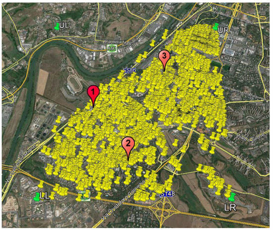
Figure 1.
Representation of the 3073 stop events in the study area.
In two previous works [12,13], a method for determining the size and position of electric charging stations in an urban area was presented, which also considered the need of the user to find a CP close to his usual destinations. The method was based on the study of traffic flows and users’ final destinations in the city of Rome. In particular, we introduced some hypothetical scenarios for the charging stations, with different numbers and distribution among stations of CPs. Figure 1 shows the position of the three charging stations (chosen from a list of traditional filling stations existing in the area and marked with red pins) used in the study. By varying the number of stations and number of charging points, it is possible to construct a multitude of scenarios.
3.1. Modeling Users Behaviour
After selecting one of the possible scenarios, we used a fuzzy model to mimic the human decision-making process of choosing a station by a user. The fuzzy method allows you to assign an "attractiveness score" to a specific station for a hypothetical BEV driver. In our work, we considered Mamdani’s fuzzy inference method, implemented in Matlab® (The MathWorks, Inc., Natick, MA, USA).
The fuzzy model used for the attractiveness score consists of the following elements:
- A.
- Input and output variablesThe input variables are (see Figure 2):
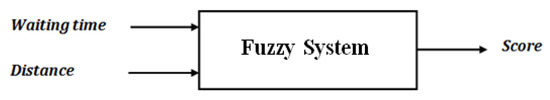 Figure 2. Input and output variables of fuzzy model.
- the waiting time for the charge event in a given station, which represents the time lapse between the parking time and the start of the charging event. This value is known to the user via some kind of communication, e.g., a mobile application. The variable values between 0 and 30 min are normalized with a linear function that varies between 0 and 10. If the waiting time is longer than 30 min, it is normalized to 10 (most disadvantageous score);
- the distance of the CI from the actual parking position. The variable is normalized with a linear function that varies between 0 (corresponding to 0 distance) and 10 (corresponding to the diagonal of the rectangular area selected), which is the most disadvantageous score.
The output is the station attractiveness score, which varies between 0 (lowest score) and 10 (highest score).
The model can in principle include other input variables that can determine the attractiveness score, but we will not examine any further parameter, for the sake of clarity of the model interpretation.
- B.
- Set of rules and membership functions (MFs).
The logic structure of the model is represented by a set of rules, while the membership functions (MFs) are the weights for the input variables, which can be expressed by any function, but must vary between 0 and 1. The function is usually chosen by the model designers on the basis of their experience. The MFs for the inputs in our case are two sigmoidal functions, which attribute a higher membership degree to lower values of the input, while for the output a triangular form was chosen as MF.
We chose a single simple rule for the model:
If (Distance is MFDis) and (Waiting time is MFWT) then (Score is MFSc).
The rule corresponds to the AND operator: the results are the minimum between the input variable values. Then, to obtain the score, the “smallest of local maximum” rule is applied, according to which the output score is identified with the abscissa of the smallest among the local maximum (see Figure 3).
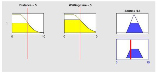
Figure 3.
Membership functions and rule of fuzzy model for the charging infrastructure (CI) score.
The fuzzy model is applied to each trip in the sample, taking into account the temporal distribution of arrivals for the entire week. The first request for a charge in the selected week coincides with the start time of the simulation. According to the fuzzy model, each charge request is assigned to a station, obtaining a list of charge requests for each CP of each CI, which is updated for each new request. The waiting time is calculated accordingly to the CP occupancy for each station. The result of the simulation is the list of charging events and the corresponding waiting times.
The results of this simulation give us an estimation of the crowding profile for the stations in each scenario, reflecting the time sequence of the charge events, and allow us to determine the level of service (LoS), which we define as being inversely proportional to the average waiting time. For a set of predefined scenarios, this method allows the best one to be defined based on the value of the ratio "(LoS) / (total number of Cps)/(number of CIs)".
For example, let us consider the scenario consisting of three stations distributed in the studied zone, as shown in Figure 1, with the following allocation of CPs: (10, 10, 20) for the stations (#1, #2, #3) respectively. Let us fix the fast charge duration in 30 min. The engagement of the CPs for this scenario is shown in Figure 4 for the entire week duration (expressed in hours). The LoS for this scenario is 94.37%.
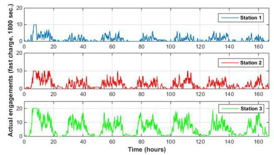
Figure 4.
Engagement at the charging points (CPs) of each CI for (10 10 20) CP distribution.
Different distributions of the CPs can change the LoS. For example, for the scenario (14, 12, 14) of CPs the LoS reduces to 87.6%. This represents a worsening compared to the (10, 10, 20) scenario due to a different redistribution of the users. Moreover, in general, lowering the total number of CPs lowers the LoS.
However, the simulations show that the dynamic of the system is quite complex, and a lower number of CPs does not always reduce the LoS. Indeed, for the distribution (8, 8, 16) the LoS is 87.7%, thus comparable to what was obtained for the previous scenario with 40 CPs. This shows that enhancing the LoS is not always necessary to increase the number of CPs.
We also investigated a different configuration of CIs. As an example, in Figure 5 we show the engagement when only stations #2 and #3 are selected, with a CP distribution (0, 12, 20). The LoS for this scenario is 89.33%, which is even higher than what was obtained for the same number of CPs distributed among three stations.
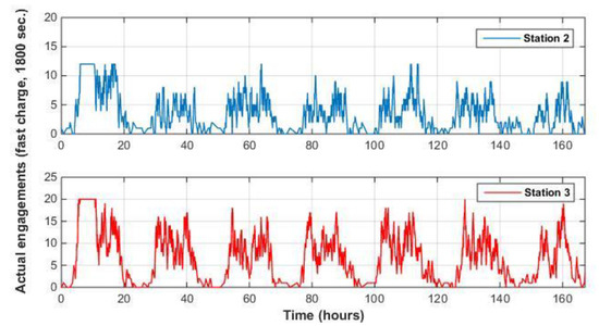
Figure 5.
Engagement at the CPs of each CI for (0 12 20) CP distribution.
Next, we analyzed the sensitivity of the model with respect to the charging duration. In Table 1 we compare the results for the maximum waiting time and LoS obtained using 30 and 23 min as charging session durations. The last value is the average of the mean values for Norway and Sweden, according to [10]. The influence of the charging session durations on the maximum waiting time is more important for the scenarios with high CP availability:

Table 1.
Comparison of maximum waiting time (WT) and LoS with variable charging duration scenarios.
As a further investigation, we considered distribution for the charging session duration. In particular, we compared four probability distributions for the average CP availability scenario (8, 8, 16):
- Poisson distribution with mean value λ = 1380;
- Weibull distribution with parameters k = 2, λ = 1;
- Weibull distribution with parameters k = 3, λ = 1;
- A simple distribution for which the charge duration is inversely proportional to the residual battery charge or depth of discharge (DoD = 1-SOC).
The Poisson distribution is a discrete probability distribution, representing the probability for the occurrence of stochastic independent events whose average time between events λ is known. For high values of λ, the Poisson distribution tends to the Gaussian distribution, which is symmetrically distributed about the mean value. The Weibull distribution is a continuous distribution that is positive only for positive values of x and is zero otherwise. It is often used in the failure analysis and is characterized by two parameters: the shape parameter k > 0, and the scale parameter λ > 0. For this distribution, the median is smaller than the mean, which is consistent with the data reported in [10]. The two distributions considered have different skewness. The last one is an empirical distribution that assumes that the higher the SOC the shorter the charge duration, which is reasonable although not always true in the real world.
All these are simple approximations of the complex charging behavior of EV users. The results for the maximum waiting time and the LoS for the proposed distributions are presented in Table 2. For options 1 to 3, the results are the mean values of 50 trials, while for option 4 we performed a single trial since it is a deterministic function.
Table 2.
Comparison of maximum WT and LoS with different probability distribution for charging duration, with mean equal to 23 min.
The Weibull distributions, which are the most left skewed among the ones considered here, show the smallest values for the maximum waiting time, as is intuitive. Surprisingly enough, the LoS, which is related to the average waiting time, does not show the highest value for the Weibull distributions but for the simple distribution proportional to the residual battery charge, which is derived from the travelled distance and under the hypothesis of a fully charged battery at the beginning of the journey. These data show the need for further investigation of the charging behavior of EV users in the CI modeling. Due to the lack of more detailed information, we will use a fixed charging duration scenario in the following, as was previously used.
The problem of charging station planning presents a contrast between the interests of investors, who aim to lower initial spending by minimizing charging points, and the users, who wish to receive the service in the shortest possible time. The overlapping of charge requests, due to a limited number of CPs, creates inconveniences for users due to long waiting times, thus reducing the LoS provided. To simulate a more realistic scenario, we add the possibility for the users to decide whether to recharge their cars or not, based on the estimated waiting time at the stations and the car battery SOC value. To this end, another fuzzy model is added to the simulation. The input values are the waiting time and the depth of discharge (DoD) of the car battery. The set of rules is represented by the single rule:
If (Waiting time is MFWT) or (DoD is MFDoD) then (Score is MFSc).
The rule and the MFs for the waiting time (MFWT), the DoD (MFDoD), and the score for the decision (MFSc) are graphically represented in Figure 6. The output of the OR operator is the maximum between the input variable values, and the operator for the defuzzifying rule is the “smallest of local maximum” of the MFSc, as was for the previous model.
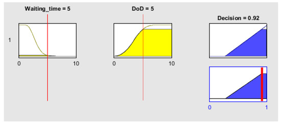
Figure 6.
Membership functions and rule of fuzzy model for charge decision.
Using this fuzzy decision model, designated as the time-out (TO) model in the following, we allow the possibility for the potential users to decide not to charge when stopping if their SOC is sufficiently high and the waiting time at the CI is too long. Conversely, if the SOC is low or there is no or little queue at the CI, the driver would charge. Table 3 and Table 4 present some figures that compare the performance of the original model with the TO one.
Table 3.
Comparison of maximum WT, LoS, and number of users lost for the models with and without time-out (TO) for 30 min charge duration.
Table 4.
Comparison of maximum WT, LoS, and number of users lost for the models with and without TO for 23 min charge duration.
For the 30 min charge duration, in all the scenarios analyzed the loss of users is around 0.9% and 2% of the total for the scenarios with high and low CP availability, respectively, and concerns primarily the peak of arrival on Monday. On the other hand, the maximum waiting time for each scenario decreases and the LoS increases, although they remain unsatisfactory in the low CP availability scenarios.
For the 23 min charge duration, the user loss is around 0.3% and 0.9% for high and low CPs availability, respectively, and the obtained level of service is always very high.
This sensitivity analysis shows that the mean duration of the charge strongly influences the model outcome. In addition, a suitable dislocation of lesser CPs can be more efficient than a larger number not satisfactorily allocated. All of these aspects should be taken into account when planning a charging infrastructure in a predefined scenario.
In the present work, the approach is completed with a detailed analysis of the power demand of a station, which is important information that influences the station performance and operation.
3.2. Fast Charging Profiles for Different SOCs
Currently, the international standards prescribe a direct current charge (Mode 4 IEC 61851-1 or SAE J1772 DC level 2) for fast (and ultra-fast) charge, because the onboard conversion would be very costly, heavy, and cumbersome.
The charging process starts from a punctual check of the conditions presented by the vehicle battery through the battery management system (BMS). This control is guaranteed by a vehicle-station communication protocol that enables charging operations after a correct recognition of the vehicle. Moreover, since the protocol structure is of the master (vehicle)‒slave (station) type, it is always the vehicle BMS that determines the battery charge conditions, according to the battery state of charge (SOC).
The fast charging profile is generally defined as a constant current-constant voltage (CC-CV) profile: at the beginning of the charge process, the battery accepts a constant current at its maximum value, set by the manufacturer and by the standard of supply (CC phase). When the voltage of the battery reaches a certain value, or when one or more cells of the package have reached a limit condition for voltage or temperature, the charging current is gradually decreased, so as to maintain the constant battery voltage (CV phase). If the initial SOC is high, the CC fraction may be short or even absent, because the battery cells quickly reach the threshold value at which the transition to CV charging takes place. The total duration of the charge will depend on a number of factors such as initial charging status, battery conditions, and temperature. The power profile of the CC-CV charge is relatively constant in the initial part and falls during the constant voltage phase, when the value of the current supplied by the battery charger decreases. The average power accepted by the battery during fast charging depends on the battery SOC.
In order to better investigate the charge power profiles for different initial SOCs and the battery behaviors, a series of experimental tests on a commercial electric vehicle of medium size (a 2014 Nissan Leaf, with a 24 kWh nominal battery capacity) was carried out at ENEA laboratories using fast charging research equipment.
The vehicle was equipped with a data acquisition system to detect the most significant battery parameters (total voltage and current, cell temperature, SOC, individual cell voltage) and road tests were conducted. A Controller Area Network (CAN) interface extracted and registered the values of interest from the CAN bus messages between vehicle and charging equipment.
The charging station used is a 50 kW CC circuitor station that uses the CHAdeMO EQC-50 standard. A LAN interface allows access to the setting and control section (see Figure 7), which are stored in a PC. The Nissan Leaf mileage is around eight thousand kilometers on urban and extra-urban roads. The relevant electrical parameters for fast charges have been recorded for several different initial SOCs, with a sampling frequency of 1 Hz.
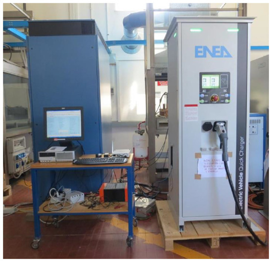
Figure 7.
The charging equipment at ENEA labs.
As an example, Figure 8a shows the battery voltage (red line) and absorbed current (blue line) for a 2000 s fast charge and initial SOC of 21%. The initial plateau for the current (constant current phase) and the subsequent rapidly decreasing current phase are clearly visible; the battery voltage shows an initial rapid growth, followed by a constant phase at the final value.
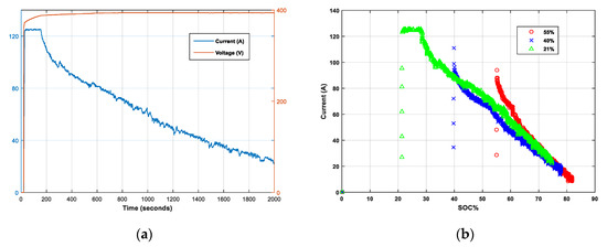
Figure 8.
(a) Battery voltage (red) and absorbed current (blue) during a fast charge, for initial state of charge (SOC) of 21%; (b) charge current profiles at three different initial SOC.
As already mentioned, at high SOC values the BMS can decide to charge the battery without the initial constant current phase. Figure 8b presents three different charging current profiles at about 21%, 40%, and 55% initial SOC and shows a variety of trends: the constant current segment is present only in the lowest SOC profile (21% SOC). The absence of the constant current phase is due to the conditions of the battery cells that require a charge current lower than the maximum deliverable from the station.
In Table 5, some electric parameters pertaining to fast charge events for another set of initial SOCs are presented. Here, Pm and PMAX are the average power and the maximum power delivered during the charge, respectively. Looking at the data, we can deduce that the battery is not fully charged after 30 min. For example, for an initial 20% SOC, corresponding to a residual energy of 4.8 kWh for the battery and considering a nominal capacity of 24 kWh, the total absorbed energy is 12.5 kWh, so the final SOC is about 72% after a 30 min fast charge.
Table 5.
Power delivered during fast charges for different initial values of the SOC.
From the measurements, we selected a set of fast charge time profiles (in terms of absorbed power per second) with initial SOCs very close to the four chosen values, 20%, 40%, 55%, 74%, and we grouped them accordingly. We then averaged the time profiles in each group in order to obtain the four average charge profiles relative to the chosen SOC values and sampled each second for a total duration of 1800 s. Next, we applied an interpolation procedure among these four reference profiles to determine the absorbed charge power relative to any SOC in the 35%–70% range of the sample. In the present work, the interpolation is done through cubic spline functions with the csapi routine in Matlab environment. Iterating the process for each timestep, we obtain the entire charging power profile over time, as shown in Figure 9, where the interpolation for SOC = 30% is reported.
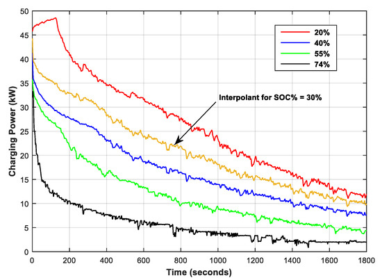
Figure 9.
The interpolated power profile for SOC = 30%.
Dedicated software in Matlab was developed in order to create a complete charge profile for the Nissan vehicle, for any given initial SOC value included in the range (35%–70%).
4. Results
In this section, an evaluation is shown of the instantaneous power load at a given CP as an effect of the charge requests. In this process, a fundamental constraint has to be respected: the sequence of the charge requests at each CP must be properly presented respecting the arrival order and avoiding overlaps during the sequential charges.
After the drivers’ charge request assignment to a CP of one of the stations in a defined scenario, according to the methodology previously illustrated, we developed a software procedure that calculates the actual SOC from the travelled distance (under the hypothesis that they started their journey with a fully charged battery). It then determines the individual charge power profiles through interpolation and, based on each parking time, properly collocates the request on the time axis of the week 6 to 12 May 2013.
We are then able to obtain the electric power load of a CP as a function of time.
We consider three stations distributed in the studied zone as shown in Figure 1, and the scenarios presented in Table 4 for a fixed charge duration of 23 min, with and without the time-out option. For each scenario illustrated in the previous section, our software procedure allows the total electric power load profile of the charging stations to be built. For the sake of simplicity, we illustrate the procedure for station #3 of each scenario.
In Figure 10 the time histories of the power load at CPs number 1, 15, and 20 pertaining to station #3 are presented for the scenario (0, 12, 20), as a result of our software procedure; the profiles are referred to Monday 6 May 2013, in the time interval 12:00 to 24:00. The individual charge power profiles are reported in chronological order, and the different form of the profiles is due to the fact that each vehicle has its own initial SOC which determines a different power absorption.
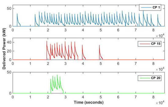
Figure 10.
Charge profiles of CP 1, 15, and 20 of station 3 for scenario (0, 12, 20).
We can observe a situation of almost complete saturation for CP number 1 and a situation of low duty for CPs number 15 and 20. In fact, according to our assignment rules of drivers to a station, the procedure saturates first the CPs of lower numbering, then moves toward the higher ones when necessary.
For comparison, Figure 11 shows the power charge profiles for CPs 1 and 15 for the scenario (0, 10, 15). The crowding level is higher, and the LoS is lower, but the power profiles are quite similar. The power between two charges does not go to zero because we assume a null switch time between two consecutive users.
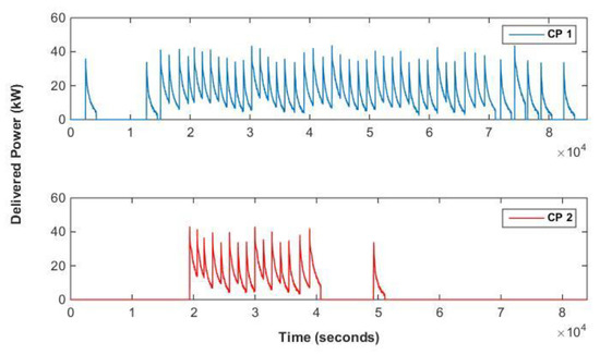
Figure 11.
Charge profiles of CP 1 and 15 of station 3 for scenario (0, 10, 15).
In Table 6 the maximum power load peak values at station #3 are reported. It can be seen that a minor availability of CP redistributes the power load in time, with the peak values of the electric power lowering with the number of CPs, but with a worsening of the LoS, as expected. The total energy supplied for the electric charges is identical in both the situations, but with a different time distribution. Except for the highest availability scenarios, there is an increase in the peak power load for station #3 when the TO is allowed. This is due to a different redistribution of the charging demand among the available charging stations. Indeed, the total energy demand is lowered when the TO for users is allowed, as can be seen in Table 7. In the model, since the charge time is the same whatever the SOC is, the service provider does not apply any SOC-based priority to the request. However, this aspect could be further investigated in business model oriented research.
Table 6.
Peak power load value at station #3 for different scenarios.
Table 7.
Weekly energy demand for the stations in different scenarios.
The sum of all the time-dependent load profiles of the CPs at station #3 gives the second by second station power load profile for the entire week.
Figure 12 and Figure 13 present the two profiles, which refer to the situations of high and low availability of CPs, respectively. It is interesting to note, by comparison between the two figures, how the latter load profile decreases and flattens out as a result of the increased time delay in serving the charge request.
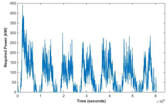
Figure 12.
The required electric power of station #3 in scenario (0, 12, 20) for the week 6 to 12 May 2013.
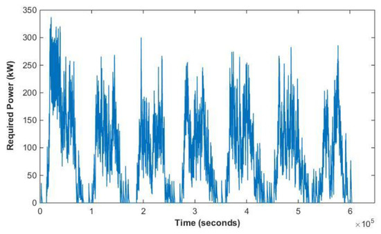
Figure 13.
The required electric power of station #3 in scenario (0, 10, 15) for the week 6 to 12 May 2013.
In Figure 14 and Figure 15, the number of drivers served by each CP of station #3 is presented by means of two bar diagrams referred to as scenario a) and scenario b), respectively.
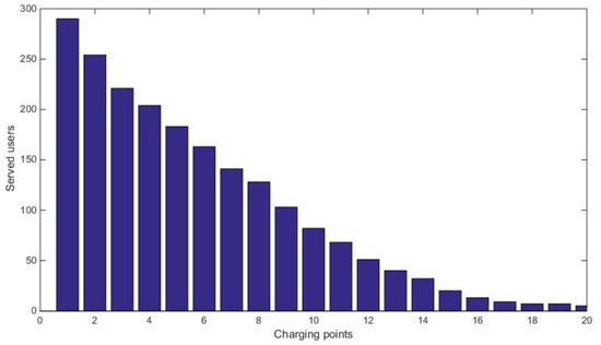
Figure 14.
Distribution among CPs of served users at station #3 in scenario (0, 12, 20).
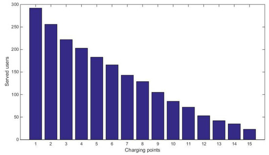
Figure 15.
Distribution among CPs of served users at station #3 in scenario (0, 10, 15).
We can note from Figure 14 how the CPs beyond number 15 for station #3 in scenario a) take a poor part in charge operations, and due to redundancy, an excellent LoS remains assured (see [13]); from Figure 15 we see that the 15 CPs of station #3 in scenario b) are more crowded. This is due to the reduction of the availability of CPs (which passes globally from 80 to 25), which does not assure an acceptable LoS, causing time overlapping between charge requests and consequent spooling (due to the assumed rule of ‘first arrived first served’).
A key strength of our methodology lies in the fact that it is easy to evaluate the ratio between the LoS (in terms of inverse of the average or maximum value of waiting time) and the level of investor profitability (depending among other things on the costs of the activated charging points); in fact, investment costs can be contained by limiting the number of CPs at the expense of the provided LoS. Another important aspect is that the output is very sensitive to the behavior model for the EV users, which needs to be thoroughly investigated.
5. Conclusions
The paper presents a methodology to evaluate the electric demand and the expected quality of service for charging infrastructure in a given scenario, based on different simulation models for users’ behavior. Several scenarios with a different number of stations and charging points have been analyzed. In general, limited availability of charging points redistributes the power load in time, resulting in a lowering of the peak power and a worsening of the quality of the service for the charging stations. Indeed, when more CPs are available, more EVs can be served at the same time, resulting in a rise of the peak demand power. We also investigated the quality of service for different distributions of CIs among the stations, which turns out to be very sensitive to the distribution of CIs and the number of total charging stations. Charging duration influences the overall level of service for any scenario, and passing from a fixed charge duration of 30 to 23 min can enhance the level of service up by 18% in the low charging points availability scenario. Furthermore, if we allow for a time distribution of charge event durations, the results show a better level of service. However, further analysis is needed to find the most appropriate distribution function. As a next step, we included the possibility for the users to decide whether to recharge their cars or not, based on the estimated waiting time at the stations and the car battery SOC value. We found that the loss of users is around 0.9% and 2% of the total for the scenarios with high and low CP availability for a fixed 30 min charge duration, which goes down to 0.3% and 0.9%, respectively, when the charge lasts 23 min. The illustrated model can be used to generate useful information in the design of a charging infrastructure scenario for BEVs, as the results may have implications on the demand side and especially on the investor side, for which the economic analysis necessary in planning new charging stations or upgrading an existing one should not ignore elements such as those presented above. In fact, in order to configure the structure of the station and the consequent economic exposure, investors must consider elements such as the attractiveness of the station, the necessary levels of electricity, and the quality of the service provided. The simulations show a highly complex dynamic of the system, which depends on many factors, sometimes in a non-linear way.
In our analysis, we hypothesized a BEV penetration of approximately 6% of the current fleet of Italian private vehicles. In a scenario of a charging infrastructure that provides high LoS, this penetration translates into the need for stations of several hundreds of kW (estimated from 300 kW to 500 kW of electric power), which represents a medium-high electric load in the context of urban areas. The rapid development of electric mobility implies an increase in the load for the stations and consequent greater demand for the electric grid. The widespread use of BEVs will increase the demand for electric power inside and outside the urban context. Consequently, it is necessary for the grid operators to implement notable structural variations to reallocate their generation points and to modify their energy distribution policies, with an increase in electric generation, integration of renewable energy sources, use of stationary storage, and a reconsideration of the distribution grid in the cities. These findings depend however on the sample chosen. With data on actual electric mobility, more realistic results can be obtained to be used in investor or policymaker analysis. Moreover, to better estimate the load demand, one should take into account the present EV market distributions and the related batteries characteristics. These points will be addressed in future work.
Author Contributions
Conceptualization, R.R. and N.A.; methodology, R.R. and N.A.; software, R.R.; validation, A.G., R.R. and N.A..; formal analysis, R.R. and N.A..; investigation, A.G.; resources, N.A.; data curation, R.R. and N.A.; writing—original draft preparation, R.R. and N.A.; writing—review and editing, A.G., R.R. and N.A.; visualization, R.R. and N.A.; supervision, A.G.; project administration, A.G.; funding acquisition, A.G. All authors have read and agreed to the published version of the manuscript.
Funding
This research was funded by Italian Ministry of Economic Development, under the project PTR 2019—21 of the Electrical System Research, Project 1.7 "Technologies for the efficient penetration of the electric vector in end uses", WP2 “Mobility”.
Conflicts of Interest
The authors declare no conflict of interest.
References
- Gnann, T.; Stephens, T.; Lin, Z.; Plotz, P.; Liu, C.; Brokate, J. What drives the market for plug-in electric vehicles?—A review of international PEV market diffusion models. Renew. Sustain. Energy Rev. 2018, 93, 158–164. [Google Scholar] [CrossRef]
- Tomaszewska, A.; Chu, Z.; Feng, X.; O’Kane, S.; Liu, X.; Chen, J.; Ji, C.; Endler, E.; Li, R.; Liu, L.; et al. Lithium-ion battery fast charging: A review. eTransportation 2019, 1, 100011–100039. [Google Scholar] [CrossRef]
- Li, W.; Long, R.; Chen, H.; Geng, J. A review of factors influencing consumer intentions to adopt battery electric vehicles. Renew. Sustain. Energy Rev. 2017, 78, 318–328. [Google Scholar] [CrossRef]
- Global EV Outlook2016—Beyond One Million ELECTRIC cars, IEA. 2016. Available online: https://webstore.iea.org/global-ev-outlook-2016 (accessed on 11 May 2020).
- Electrifying Insights: How Automakers can Drive Electrified Vehicle Sales and Profitability, McKinsey’s Report. Available online: https://www.mckinsey.com/~/media/McKinsey/Industries/Automotive%20and%20Assembly/Our%20Insights/Electrifying%20insights%20How%20automakers%20can%20drive%20electrified%20vehicle%20sales%20and%20profitability/Electrifying%20insights%20-%20How%20automakers%20can%20drive%20electrified%20vehicle%20sales%20and%20profitability_vF.ashx (accessed on 11 May 2020).
- Gnann, T.; Funke, S.; Jakobsson, N.; Plotz, P.; Sprei, F.; Plotz, P. Fast charging infrastructure for electric vehicles: Today’s situation and future needs. Transp. Res. Part D: Transp. Environ. 2018, 62, 314–329. [Google Scholar] [CrossRef]
- Nicholas, M.; Tal, G.; Woodjack, J. California Statewide Charging Assessment Model for Plug-in Electric Vehicles: Learning from Statewide Travel Surveys, Institute of Transportation Studies, Working Paper Series, Institute of Transportation Studies, UC Davis. 2013. Available online: https://EconPapers.repec.org/RePEc:cdl:itsdav:qt3qz440nr (accessed on 11 May 2020).
- Blythe, P.T.; Neaimeh, M.; Serradilla, J.; Pinna, C.; Hill, G.; Guo, A. Rapid Charge Network Activity 6 Study Report. 2015. Available online: https://rapidchargenetwork.com/resources/ (accessed on 11 May 2020).
- Neaimeh, M.; Salisbury, S.D.; Hill, G.A.; Blythe, P.; Scoffield, D.R.; Francfort, J.E. Analysing the usage and evidencing the importance of fast chargers for the adoption of battery electric vehicles. Energy Policy 2017, 108, 474–486. [Google Scholar] [CrossRef]
- Figenbaum, E. Charging into the Future—Analysis of Fast Charger Usage; TØI Report, 1682/2019; 2019; ISBN 978-82-480-2214-5. Available online: https://www.toi.no/getfile.php?mmfileid=49751 (accessed on 11 May 2020).
- Nicholas, M.; Hall, D. Lessons Learned on Early Electric Vehicle Fast-Charging Deployments, White Paper, The international Council on Clean Transportation. 2017. Available online: https://theicct.org/sites/default/files/publications/ZEV_fast_charging_white_paper_final.pdf (accessed on 11 May 2020).
- Andrenacci, N.; Ragona, R.; Valenti, G. A demand-side approach to the optimal deployment of electric vehicle charging stations in metropolitan areas. Appl. Energy 2016, 182, 39–46. [Google Scholar] [CrossRef]
- Andrenacci, N.; Genovese, A.; Ragona, R. Determination of the level of service and customer crowding for electric charging stations through fuzzy models and simulation techniques. Appl. Energy 2017, 208, 97–107. [Google Scholar] [CrossRef]
- Morrissey, P.; Weldon, P.; O’Mahony, M. Future standard and fast charging infrastructure planning: An analysis of electric vehicle charging behaviour. Energy Policy 2016, 89, 257–270. [Google Scholar] [CrossRef]
- Huang, X.; Li, X.; Yuan, X.; He, B.; Li, J. An Economic Evaluation of Electric Vehicle Charging Infrastructure in Public Places in China. IOP Conf. Series: Earth Environ. Sci. 2018, 168, 012018. [Google Scholar] [CrossRef]
- Narassimhan, E.; Johnson, C. The role of demand-side incentives and charging infrastructure on plug-in electric vehicle adoption: Analysis of US States. Environ. Res. Lett. 2018, 13, 74032–74043. [Google Scholar] [CrossRef]
- Babic, J.; Carvalho, A.; Ketter, W.; Podobnik, V. Electricity Trading Agent for EV-enabled Parking Lots. In Agent-Mediated Electronic Commerce. Designing Trading Strategies and Mechanisms for Electronic Markets; Ceppi, S., David, E., Hajaj, C., Robu, V., Vetsikas, I., Eds.; Springer: Berlin/Heidelberg, Germany, 2017; Volume 271. [Google Scholar]
- Pevec, D.; Babic, J.; Kayser, M.A.; Carvalho, A.; Ghiassi-Farrokhfal, Y.; Podobnik, V. A data-driven statistical approach for extending electric vehicle charging infrastructure. Int. J. Energy Res. 2018, 42, 3102–3120. [Google Scholar] [CrossRef]
- Sadeghi-Barzani, P.; Rajabi-Ghahnavieh, A.; Kazemi-Karegar, H. Optimal fast charging station placing and sizing. Appl. Energy 2014, 125, 289–299. [Google Scholar] [CrossRef]
- Hanabusa, H.; Horiguchi, R. A Study of the Analytical Method for the Location Planning of Charging Stations for Electric Vehicles. In Knowledge-Based and Intelligent Information and Engineering Systems; König, A., Dengel, A., Hinkelmann, K., Kise, K., Howlett, R.J., Jain, L.C., Eds.; Springer: Berlin/Heidelberg, Germany, 2011; Volume 6883. [Google Scholar]
- Davidov, S.; Pantoš, M. Planning of electric vehicle infrastructure based on charging reliability and quality of service. Energy 2017, 118, 1156–1167. [Google Scholar] [CrossRef]
- Zhang, Y.; Qiu, Z.; Gao, P.; Jiang, S. Location model of electric vehicle charging stations. J. Physics: Conf. Ser. 2018, 1053, 12058–12065. [Google Scholar] [CrossRef]
- Xiang, Y.; Liu, J.; Li, R.; Li, F.; Gu, C.; Tang, S. Economic planning of electric vehicle charging stations considering traffic constraints and load profile templates. Appl. Energy 2016, 178, 647–659. [Google Scholar] [CrossRef]
- Mu, Y.; Wu, J.; Jenkins, N.; Jia, H.; Wang, C. A Spatial—Temporal model for grid impact analysis of plug-in electric vehicles. Appl. Energy 2014, 114, 456–465. [Google Scholar] [CrossRef]
- Ma, C.-T. System Planning of Grid-Connected Electric Vehicle Charging Stations and Key Technologies: A Review. Energies 2019, 12, 4201. [Google Scholar] [CrossRef]
- Labeye, E.; Hugot, M.; Brusque, C.; Regan, M.A. The electric vehicle: A new driving experience involving specific skills and rules. Transp. Res. Part F: Traffic Psychol. Behav. 2016, 37, 27–40. [Google Scholar] [CrossRef]
- Rolim, C.; Gonçalves, G.; Farias, T. Rodrigues, Óscar Impacts of Electric Vehicle Adoption on Driver Behavior and Environmental Performance. Procedia - Soc. Behav. Sci. 2012, 54, 706–715. [Google Scholar] [CrossRef]
- Pan, L.; Yao, E.; Zhang, R. Location Model of EV Public Charging Station Considering Drivers’ Daily Activities and Range Anxiety: Case Study of Beijing. In Proceedings of the Transportation Research Board 96th Annual Meeting Proceeding, Washington, DC, USA, 8–12 January 2017. [Google Scholar]
- González, J.; Alvaro, R.; Gamallo, C.; Fuentes, M.; Fraile-Ardanuy, J.; Knapen, L.; Janssens, D. Determining Electric Vehicle Charging Point Locations Considering Drivers’ Daily Activities. Procedia Comput. Sci. 2014, 32, 647–654. [Google Scholar] [CrossRef]
- Iversen, E.B.; Morales, J.M.; Madsen, H. Optimal charging of an electric vehicle using a Markov decision process. Appl. Energy 2014, 123, 1–12. [Google Scholar] [CrossRef]
- Ramesh, K.; Bharatiraja, C.; Raghu, S.; Vijayalakshmi, G.; Sambanthan, P. Design and Implementation of Real Time Charging Optimization for Hybrid Electric Vehicles. Int. J. Power Electron. Drive Syst. (IJPEDS) 2016, 7, 1261–1268. [Google Scholar] [CrossRef]
- Chokkalingam, B.; Padmanaban, S.; Siano, P.; Ramesh, K.; Selvaraj, R. Real-Time Forecasting of EV Charging Station Scheduling for Smart Energy Systems. Energies 2017, 10, 377. [Google Scholar] [CrossRef]
- Tan, K.M.; Ramachandaramurthy, V.K.; Yong, J.Y. Integration of electric vehicles in smart grid: A review on vehicle to grid technologies and optimization techniques. Renew. Sustain. Energy Rev. 2016, 53, 720–732. [Google Scholar] [CrossRef]
- Bayram, I.S.; Michailidis, G.; Devetsikiotis, M.; Granelli, F. Electric Power Allocation in a Network of Fast Charging Stations. IEEE J. Sel. Areas Commun. 2013, 31, 1235–1246. [Google Scholar] [CrossRef]
- Cheon, S.; Kang, S.-J. An Electric Power Consumption Analysis System for the Installation of Electric Vehicle Charging Stations. Energies 2017, 10, 1534. [Google Scholar] [CrossRef]
- Evaluating Electric Vehicle Charging Impacts and Customer Charging Behaviors: Experiences from Six Smart Grid Investment Grant Projects; U.S. Department of Energy Office of Electricity Delivery and Energy Reliability: Washington, DC, USA, 2014.
- Octo Group S.p.A. Available online: https://www.octotelematics.com/it/home-page-it/ (accessed on 11 May 2020).
- Electric Vehicle range. Available online: https://www.ergon.com.au/network/smarter-energy/electric-vehicles/electric-vehicle-range (accessed on 11 May 2020).
- Philipsen, R.; Brell, T.; Biermann, H.; Ziefle, M. Under Pressure—Users’ Perception of Range Stress in the Context of Charging and Traditional Refueling. World Electr. Veh. J. 2019, 10, 50. [Google Scholar] [CrossRef]
- Björnsson, L.-H.; Karlsson, S. Electrification of the two-car household: PHEV or BEV? Transp. Res. Part C: Emerg. Technol. 2017, 85, 363–376. [Google Scholar] [CrossRef]
- Niklas, U.; von Behren, S.; Chlond, B.; Vortisch, P. Electric Factor—A Comparison of Car Usage Profiles of Electric and Conventional Vehicles by a Probabilistic Approach. World Electr. Veh. J. 2020, 11, 36. [Google Scholar] [CrossRef]
© 2020 by the authors. Licensee MDPI, Basel, Switzerland. This article is an open access article distributed under the terms and conditions of the Creative Commons Attribution (CC BY) license (http://creativecommons.org/licenses/by/4.0/).