Article

Energy Use and Labor Productivity in Ethiopia: The Case of the Manufacturing Industry

by
Selamawit G. Kebede
1 and
Almas Heshmati
2,*
1
Department of Economics, Addis Ababa University, Main campus at 6 Kilo, Addis Ababa, Ethiopia
2
Jönköping International Business School, P.O. Box 1026, SE-551 11 Jönköping, Sweden
*
Author to whom correspondence should be addressed.
Energies 2020, 13(11), 2714; https://doi.org/10.3390/en13112714
Submission received: 9 April 2020 / Revised: 10 May 2020 / Accepted: 26 May 2020 / Published: 28 May 2020
(This article belongs to the Collection Energy Use Efficiency)

Abstract

:
This study investigates the effect of energy use on labor productivity in the Ethiopian manufacturing industry. It uses panel data for the manufacturing industry groups to estimate the coefficients using the dynamic panel estimator. The study’s results confirm that energy use increases manufacturing labor productivity. The coefficients for the control variables are in keeping with theoretical predictions. Capital positively augments productivity in the industries. Based on our results, technology induces manufacturing’s labor productivity. Likewise, more labor employment induces labor productivity due to the dominance of labor-intensive manufacturing industries in Ethiopia. Alternative model specifications provide evidence of a robust link between energy and labor productivity in the Ethiopian manufacturing industry. Our results imply that there needs to be more focus on the efficient use of energy, labor, capital, and technology to increase the manufacturing industry’s labor productivity and to overcome the premature deindustrialization patterns being seen in Ethiopia.

1. Introduction

Industrial expansion is essential for socioeconomic development as it generates different opportunities—capital accumulation, structural changes, technological innovations, and productivity—that improve economic performance [1,2,3]. Industrialization or the shift from agriculture to the manufacturing sector is key to development, making development without industrialization an unthinkable process [1,4]. Industrial development is also the pathway for the structural transformation of an economy and society. High rates of economic growth and capital accumulation are essential but not adequate for structural transformation, unless complemented by industrialization [2]. Industrialization promotes economic diversification, inclusive growth, and the efficient utilization of resources, such as physical, human, and mineral resources, which help eradicate poverty [5].
The productivity advantage of manufacturing over other sectors is a major factor for pursuing sustained industrialization, along with the higher externalities that can arise from manufacturing growth [6]. Unlike agriculture and the service sectors, manufacturing accelerates convergence and, with its huge productivity advantages, will enable developing economies to catch up with their developed counterparts [4]. Different factors are attributed to industrial growth and productivity, including human or physical capital, labor, energy, innovations, and capacity utilization [3,7,8]. Among others, energy is critical for productivity and growth as it enables achieving both industrial development and structural transformation [9]. In fact, the use of energy is a precondition for the development of human society and more energy use is required for sustaining industrial development [9]. Energy use is directly related to growth and economic development and is an essential input for all production and consumption activities [8,10].
The causal relationship between energy consumption and growth has been investigated in different countries but the results remain controversial with diverse outcomes in different countries based on the econometric approaches used and the time spans of the studies [10,11,12,13,14]. Some studies validate the positive effects of energy on growth and productivity [15,16,17], while others empirically confirm a negative impact of energy on growth and productivity [11,12]. Others find no causal relationship between the two empirically [10,18]. Here we use different econometric estimators for matters of sensitivity analysis of the result to evaluate how energy affects labor productivity in Ethiopian manufacturing.
In Ethiopia, the share of agriculture and services in gross domestic product (GDP) has been more than 60 percent and 20 percent, respectively, for decades, while manufacturing’s contribution to GDP has been less than five percent, which, too, is attributable to other industries [19,20]. Currently, the service sector contributes 47 percent, agriculture 43 percent, and industry makes up the rest, leaving a very low share of GDP being contributed by manufacturing [21]. The existing literature confirms that Ethiopian people have been depending on agriculture for their livelihood for decades in terms of production and employment, with significantly small contributions from the manufacturing sector to the economy [22,23]. The dominance of, first, the agriculture sector and, later, the service sector shows premature deindustrialization in Ethiopia, while the low share of manufacturing implies output deindustrialization [21,24].
The low industry performance can be attributed to several factors such as inefficient use of labor, energy, human or physical capital, innovations and capacity utilization [3,8,24]. As established theoretically, energy is a significant factor in determining sustainable industrial production. However, the empirical relationship between energy and growth is mixed [10,11,12,13,14]. Besides, there are very few empirical studies on energy and productivity at the industry level. This motivated us to undertake this study on the empirical relationship between energy and labor productivity in the case of the Ethiopian manufacturing industry. Accordingly, this study addresses the following research question:
How does energy effect labor productivity in the Ethiopian manufacturing industry?
The analysis emphasizes the role of energy use in manufacturing labor productivity in Ethiopia. The study uses panel data for estimating the empirical model using a dynamic generalized method of moments (GMM) estimator. The estimation results confirm that energy use positively effects labor productivity in the manufacturing sector in Ethiopia. This implies that the efficient use of energy is a pillar of labor productivity in the Ethiopian manufacturing industry. Thus, this study adds to the existing literature by empirically confirming the relationship between energy use and labor productivity across different model specifications.
The rest of this research is organized as follows. Section 2 reviews the literature on energy and productivity. The empirical model and estimation approach are presented in Section 3, along with the definitions of the variables used in the model. Data are discussed in Section 4. A descriptive and regression-based analysis of the energy and labor productivity of the manufacturing sector in Ethiopia is discussed in Section 5. The final section gives the conclusion and the implications of the findings.

2. Literature Review on Energy and Productivity Growth

This section presents a general overview of the link between energy and productivity, followed by an empirical review of the relationship between energy and growth. It then discusses existing studies on the determinants of labor productivity. This helps establish the rationale for undertaking this study that links energy with labor productivity at the industry level in Ethiopia.
There are two empirically fundamental questions related to disparities in the level of economic development across nations. Economists inquire why some economies are richer than others, and what accounts for the huge increases in real incomes over time [25,26]. The extensive dispersion of output growth rates across countries is documented economically [27]. A comparison between countries shows that countries that at one time had similar levels of per capita income consequently followed very different patterns, with some seemingly caught in long-term stagnation while others were able to sustain high growth rates [28].
Among others, productivity is a determining factor of growth at the national and industrial levels, with increasing globalization and the expansion of competitive industrial product markets [16,29]. High industrial labor productivity results in lower per unit costs and increases firms’ ability to compete in global markets [16]. There are several determinants of labor productivity, including human or physical capital, energy, and technology [29,30,31]. Energy is an essential input that constrains or induces productivity growth in different firms. It is an essential factor of production that is required in all economic processes [29,31]. This basic production input in economic activities provides a conducive platform for industrial growth and productivity. The efficient use of energy leads to the higher productivity of resources and a more dynamically competitive economy that can respond to the required economic transition from agriculture to industry dominated structure [32].
Energy has countless ways of empowering human beings through increasing productivity, powering industrial and agricultural processes, alleviating poverty, and facilitating sound social and economic development [33]. Limited access to energy cripples economic growth and development, which makes universal access to energy a major emphasis of the sustainable development goals [9]. The increased availability and use of energy increases productivity and enhances economic development [34]. Energy is primarily associated with the provision of power for agricultural or industrial production [35,36]. In fact, sustainable development and modern industry require reliable, affordable, and energy services available for all on a sustainable basis [9,33]. However, access to energy is limited and is accompanied by low quality and poor reliability, affordability, and availability [9]. Energy can be measured in terms of cost or value and can be disaggregated into electricity or other forms of energy based on types. It is possible to measure energy consumption in equivalent kilowatt hours (KWh) [37].
Energy use is a major stimulating factor in industrial productivity [16,32]. Public services and industrial production require access to energy use [12]. Recently, the demand for energy has been increasing, with the world having a population of over 7.2 billion, which is increasing [38]. Access to energy in Africa is low—for every ten people in sub-Saharan Africa (SSA), only four have access to electricity compared to the global access of nine out of ten people having access to energy; 57 percent of the global deficiency in access to electricity energy comes from SSA [9].
There is an increasing interest in identifying energy’s role in productivity, as empirical findings on their causal relationship are mixed [13,39]. For instance, Schurr et al. [40] presents the association between energy consumption and growth in the national product (GNP) in the United States over the period 1880-1955. These authors identified two trends in the pattern of the energy share in relation to GNP. The share of energy to GNP was rising, until it declined persistently after the war. This change in the trend is attributed to a compositional change in the national output to light industries, which use less energy compared to heavy manufacturing industries and services and is also due to major improvements in the efficiency of energy conservation in light industries. In a follow-up to the study by Schurr et al. [40], Schurr [41] explored the link between energy use, productive efficiency, and energy efficiency from the 1920s to 1981. His study indicated that energy intensity, defined as energy’s share in GNP, declined when multifactor productivity increased during the study period. Unlike the share of energy in output, which is attributed to technological advances that increased overall productive efficiency, energy intensities in terms of factor inputs increased over the study period. This ultimately led to an increase in the final output, which was more than the consumption of energy.
The role of electrification and non-electricity energy in productivity growth for the USA’s economy is examined by Jorgenson [42]. His study confirms that electricity energy is related to productivity growth. However, there is also a strong association between non-electricity energy and productivity growth in the US economy. In another related study, Boudreaux [43] examined the impact of electricity energy on manufacturing productivity in the US from 1950 to 1984. This study showed that growth in electricity energy accounted for 79 percent of the value added to the manufacturing sector. Empirically, the study showed that the decline in energy growth accounted for the slowdown in productivity and output growth.
The role of energy in productivity growth in the European Union countries is assessed by Murillo-Zamorano [44] who empirically confirmed that energy is a fundamental input in productivity change. In another related study, the relationship between energy and labor productivity was examined by studying the effect of renewable and non-renewable energy in European countries over the period from 1995 to 2015 using the production frontier approach [45]. This study showed that renewable and non-renewable energy had an effect on the growth of the countries in the European Union. Based on his study, the author concluded that non-renewable energy had a positive impact, leading to divergence, while renewable energy had a negative impact, leading to convergence.
Energy and income causality for ten emerging markets, excluding China because of limited data availability and the G-7 countries, is examined in Soytas and Sari [17]. Their results show the bidirectional causality in Argentina, causality running from energy to GDP in France, Germany, Japan, and Turkey and causality running from GDP to energy consumption in Italy and Korea. The nexus between energy and growth for 20 net importer and exporter countries from 1971 to 2002 using the panel vector correction model is investigated by Mahadevan and Asafu-Adjaye [46]. Their findings show that for energy exporter developed countries this causal relationship is bidirectional, while for developing countries energy stimulates growth in the short term.
The effect of energy consumption and human capital on economic growth for 130 oil-exporting and developed countries from 1981 to 2009 is investigated by Alaali et al. [15]. Using GMM, they estimate an augmented neoclassical growth model, including education and health as human capital along with energy consumption. Their results show that energy had a positive and significant effect on growth. The empirical relationship between energy consumption and gross domestic product for six Gulf Cooperation Council (GCC) countries using cointegration and causality methods is investigated by Al-Irani [13]. His results show a unidirectional causal relationship running from GDP to energy consumption, but not the other way around. Moghaddasi [11] investigated the role of energy consumption in total-factor productivity in Iranian agriculture using the Solow residual model and their results show a negative impact, which they attribute to cheap and inefficient use of energy in this sector.
Kebede et al. [12] investigated energy demand in east, west, central, and south sub-Saharan countries using time series cross-sectional data for 20 countries for a 25-year time span. Their results show that energy demand was positively related to GDP, the population growth rate, and agricultural expansion, while it was negatively correlated with industrial development and the price of petroleum. The causal relationship between energy consumption and economic growth for 11 sub-Saharan African countries is investigated by Skinlo [18] using the ARDL bound test and Granger causality. His results show that there was cointegration between energy use and economic growth in seven countries included in the study: Ghana, Cameron, Senegal, Cote d’Ivoire, Zimbabwe, Gambia, and Sudan. In Sudan and Zimbabwe, the Granger causality ran from economic growth to energy use while in Cameroon and Cote d’Ivoire he found no Granger causality between energy consumption and economic growth.
Wolde-Rufael [39] investigated the causal relationship between energy consumption and economic growth for 17 African countries using the variance decomposition factor and impulse response analysis. The variance decomposition analysis confirmed that labor and capital were important, while energy was not as important as these factors. A meta-analysis using a multinomial logit model for 174 samples was conducted by Chen et al. [10] to explore the relationship between energy and GDP, with controversial results that show that the time span, econometric model, and selection characteristics affected the debatable outcomes of the casual relationship significantly.
The second part of this section explores labor productivity and its determinants, as studied by different researchers. Su and Heshmati [30] studied the development and source of labor productivity in 31 provinces of China during 2000-09. They used a fixed effects model adjusted for heteroscedasticity to estimate the coefficients’ fixed assets, average labor wage, total volume of business, post and telecommunications, and profits, which had a positive effect on labor productivity. Accounting for heterogeneity, Velucchi and Viviani [47] examined the determinants of labor productivity in Italian firms using panel data and a quantile regression. Their results show that human capital and assets had a strong positive impact on fostering the productivity of low productive firms compared to high productive ones. Islam and Syed-Shazali [48] studied the impact of the degree of skills, research and development (R&D), and a favorable work environment on the productivity of labor-intensive manufacturing industries in Bangladesh. Their results confirmed a positive correlation between productivity and the degree of skills and the work environment, though it was a weak correlation; R&D had a strong positive correlation with productivity in Bangladesh.
Recently, Heshmati and Rashidghalam [49] studied the determinants of labor productivity in manufacturing and service sectors in Kenya using the World Bank Enterprise Survey database for 2013. Their findings confirm a positive effect of capital intensity and wages on labor productivity while female participation reduced productivity in these sectors. In a comparative study, Nagler and Naudé [50] examined the factors determining the labor productivity of non-farm enterprises in rural sub-Saharan Africa in Ethiopia, Nigeria, Uganda, and Malawi using the World Bank’s Living Standards Measurement Study – Integrated Surveys on Agriculture (LSMS-ISA) database. They found that rural enterprises were less productive than urban enterprises. By estimating Heckman selection and using panel data models, their study confirmed that education and credit availability induced enterprises’ labor productivity.
Samuel and Aram [51] studied the main factors that helped or hindered the realization of industrial productivity in Africa. The study concluded that financial development, economic development, the labor market’s flexibility, and the real effective exchange rate were clear determinants of industrialization in the entire region. In a time-series analysis Otalu and Anderu [7], the determinants of industrial sector growth in Nigeria were examined using the cointegration and error correction model (ECM). Their results show that both labor and capital had significant effects on economic growth. The exchange rate showed a positive and significant impact, signifying that currency appreciation might be detrimental to the growth of the industrial sector. In addition, the authors also found that these factors had a more permanent and not a transitory effect on industrial output.
In the energy literature, the contribution of energy use to productivity in practice is controversial, with some studies claiming that energy use is a fundamental pillar of productivity growth, while others argue that energy has little effect on productivity growth [10,44]. In studies on labor productivity, energy seems to be missing as a major determinant factor in explaining labor productivity [47,48,49,50,51]. Furthermore, there is little focus on investigating the explicit role of energy in labor productivity from the manufacturing industry’s perspective [47,48,49]. Most growth theories fail to include energy use as a pillar of productivity or as one argument for the growth differences between nations [45].
Thus, this study adds to the existing literature by addressing the controversial nature of previous studies’ results by empirically investigating the association between energy and productivity in the Ethiopian manufacturing industry. It also considers energy as a major variable of interest for explaining labor productivity in addition to capital and technical changes. This link is investigated from the manufacturing industry’s perspective. Moreover, this study uses different model specifications to confirm the consistency of this relationship by using both static and dynamic panel data estimators for the manufacturing industry groups.

3. Model Specification and Estimation

3.1. Model Specification

Productivity is a fundamental indicator for assessing economic performance [52]. In general terms, productivity can be defined as the ratio of total output produced to the inputs used. There are different measures of productivity, which can be classified as multifactor productivity measures and single factor measures of productivity [53]. The former relate output to a bundle of inputs, while the latter measure the ratio of output to a single input [52]. For instance, labor productivity is defined as the ratio of the quantity index of gross output to the quantity index of labor input [53]. Among other factors, energy is a key driver of economic growth and industrialization as it enhances the productivity of labor, capital, and other factors of production. In fact, energy use has received considerable attention as a pillar of productivity in the literature on energy economics, but with mixed empirical results for different countries on the causal relationship between the two [13,15,46].
This study empirically investigates the relationship between energy use and labor productivity in Ethiopian manufacturing industries. Like labor and capital production factors, energy is seen as an essential factor for economic development [15]. The production function is a useful tool for analyzing the technological relationship between labor, capital, other inputs, and the output produced [54]. The production function which relates output to the vector of inputs is mostly used for analyzing productivity [55,56]. Accordingly, in this study, the production function developed by Cobb and Douglas [57] is used for estimating the productivity of labor in the manufacturing sector in Ethiopia. The Cobb–Douglas production function, with two inputs in its basic form [58,59], is represented as:
Y = AL α K β
where Y denotes the quantity of production or output or its value, L represents labor or its value, and K stands for the value of capital. α and β are parameters of inputs labor and capital respectively and A is technology. This standard production function can be generalized to include more inputs such as energy and other material inputs:
Y = AL α K β E γ
where the other variables are defined in the same manner as in Equation (1). E stands for energy inputs in the production process and γ denotes a parameter to be estimated as a coefficient for energy input. We can linearize the production function by log transformation as:
LogY = logA + α logL + β logK + γ logE + U
if   α + β + γ > 1 , IRS if   α + β + γ 1 , DRS if   α + β + γ = 1 , CRS
where α, β, and γ stand for elasticities of production with respect to labor, capital, and energy respectively. Equation (3) is the first model to be estimated to decide production’s returns to scale in the manufacturing industry in Ethiopia. The sum of the parameters will give us a measure of the returns to scale from a proportional increase in inputs. If the sum of the parameters is greater than one we have increasing returns to scale (IRS); if the sum is less than one, we get decreasing returns to scale (DRS); if the sum is one then the returns to scale are constant (CRT).
As labor productivity shows how effectively labor inputs are converted into outputs [60], we take production or output per employee to measure labor productivity. There are two ways of doing this. First, if one is interested in the scale effects of energy and capital use on labor productivity, then the right-hand side of the equation to include all inputs in the original form per labor, while the left side is measured as productivity—that is, output is divided by labor. In this case, labor, on the right-hand side, represents the scale of production as:
Y L = AL α K β E γ L
Y / L = AL α 1 K β E γ
LogY / L it = logA it + ( α 1 ) logL it + β logK it + γ logE it + U it
ρ = α 1 ; then , α = ρ + 1
LogY / L it = λ + ρ logL it + β logK it + γ logE it + t it + U it
where the dependent variable is labor productivity, which measures the scale effect of the factors on labor productivity. Value of energy is used for the manufacturing industry as a major variable of interest. Labor is a control variable that represents the scale of production and is defined as the number of employees in the industry group. The second key control variable is capital, which is defined as the value of the industry groups’ fixed assets. All variables are in logarithm form, so that the coefficients are defined elasticities. T represents the trend, which is included for capturing the technical change effect. U represents the error term of the panel model and subscripts i and t represent the industry sector and time period respectively. U contains unobservable sector- and time-specific effects. βs are unknown coefficients of the explanatory variables, where λ is the constant term.
Equations (6a) and (6b) represent the third model, which measures the intensity effect of factors on labor productivity. The other way of specifying the model is by dividing the right-hand side variables (L, K, E) with labor to express energy and capital in the form of capital intensity and energy intensity, respectively, while the L ratio will end up in the intercept. Thus, the third model to be estimated is written as:
Y L = ( A L ) ( L L ) α ( K L ) β ( E L ) γ
Y L = ( A L ) ( K L ) β ( E L ) γ ; ( L L ) α = 1 α = 1
For all the three models to be estimated, an error term is included and the models are linearized and transformed into logarithm forms before estimation. The third model to be estimated (7a) measures energy and capital intensity and their effect on labor productivity in manufacturing industrial groups in Ethiopia:
Log ( Y / L ) it = μ + β logk it + γ loge it + t it + u it
LogMLP it = α + β logCapital   Intensity it + γ logEnergy   Intensity it + λ trend it + U it
where manufacturing labor productivity is the dependent variable defined as the manufacturing output of an industry group per employee. µ is the intercept, β is a slope coefficient for capital intensity, γ is a slope coefficient for energy intensity, while t stands for time trend to represent a shift in the production function over time and thus λ is the rate of technological change. U is the error term in the model with i and t representing industry group and time respectively. It follows an error component structure consisting of industry effects and random error components.

3.2. Model Estimation

Panel data models can be static or dynamic. Static panel data models can be estimated using pooled ordinary least squares (OLS), fixed effects (FE), and random effects (RE) models, but these models do not take the problems of heteroscedasticity, serial correlation, and the endogeneity of the explanatory variables into account [61,62,63]. The pooled OLS model ignores fixed industry and time effects. In FE, these are fixed effects correlated with the inputs, while it is assumed that they do not correlate with inputs in the RE model. In all the models, the time effects are captured by the trend. In the FE model, we estimate the effects in the form of industry intercepts, while, in RE, we estimate the parameters of the distribution of the industry effects which, are assumed to have means of zero and constant variance [63].
To solve the estimation problems related to a static panel formulation, we use the dynamic panel model of difference GMM and system GMM estimators, as proposed by Arellano Bond [64] and Arellano and Bover [65], respectively. The difference GMM and system GMM are dynamic panel estimators designed for large N and small T, many groups/individuals, a few time periods, a linear functional relationship, one left-hand side that is dynamic depending on its own past realization, and for independent variables that are not strictly exogenous [66]. System GMM contains both level and first difference equation parts, it uses instruments in levels for equations in first difference and uses instruments in first difference for equations in levels [61]. After estimating the dynamic panel data models, tests for the serial correlation of the residuals and overidentification were done using Hausman or Sargan tests and the autoregressive AR (2) test, respectively [64,65].

4. The Data

4.1. Data and Variables

All data used in this study are taken from the Ethiopian Central Statistical Authority (CSA). The period 2005–2016 is chosen for the study since the latest information on all variables is available only up to 2016. The number of industry groups and the study period were determined by data availability. A two-digit industry sector level is the most disaggregated data level available for this specific case. The number of observations for industry groups (industrial sectors) is 15, where, for every industry group, the relevant variables available are included. Table 1 provides a list of the industry groups. The medium and large manufacturing industries in Ethiopia are categorized into 15 industry groups.
Table 2 gives the list of variables used in this study and their definitions. To define labor productivity, we need information on production and employment. Production, in our case, is defined as the gross value of production by industry group. Employment is defined as the number of employees by industry group. Accordingly, labor productivity is defined as the ratio of production to employment by industry group or per capita employed production, labeled in the literature as labor productivity. Energy is defined as the ratio of the value of energy consumed by the industry groups. Capital is defined as the total value of the fixed assets by industry groups. Table 2 also shows the expected effects of the variables in the model on labor productivity. Labor productivity is the dependent variable and the explanatory variables are energy use, employment, capital, and trend which are expected to be statistically significant in the empirical estimation. The expected sign for employment is positive as industries in Ethiopia are more labor intensive, so adding more labor is expected to increase production. Similarly, the expected signs of the parameters for energy, capital, and technical change are expected to be positive. It is assumed that energy use and capital will increase labor productivity in the manufacturing industries in Ethiopia. Wages and salaries were included as a proxy for human capital but they were excluded from the estimation due to high collinearity problem. An increase in wages and salaries is expected to positively affect labor productivity and higher wages per capita reflect the laborers’ skills and education levels.

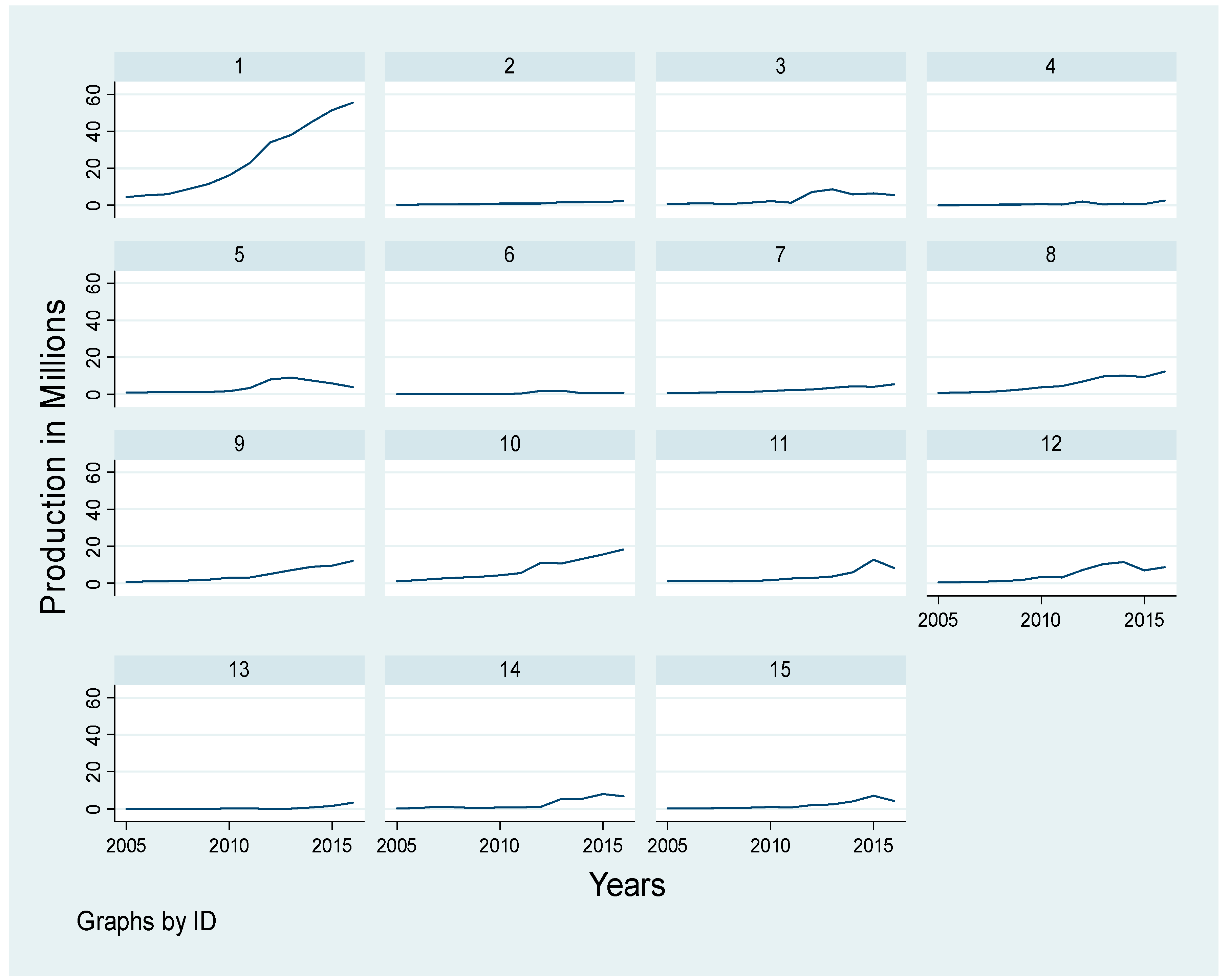
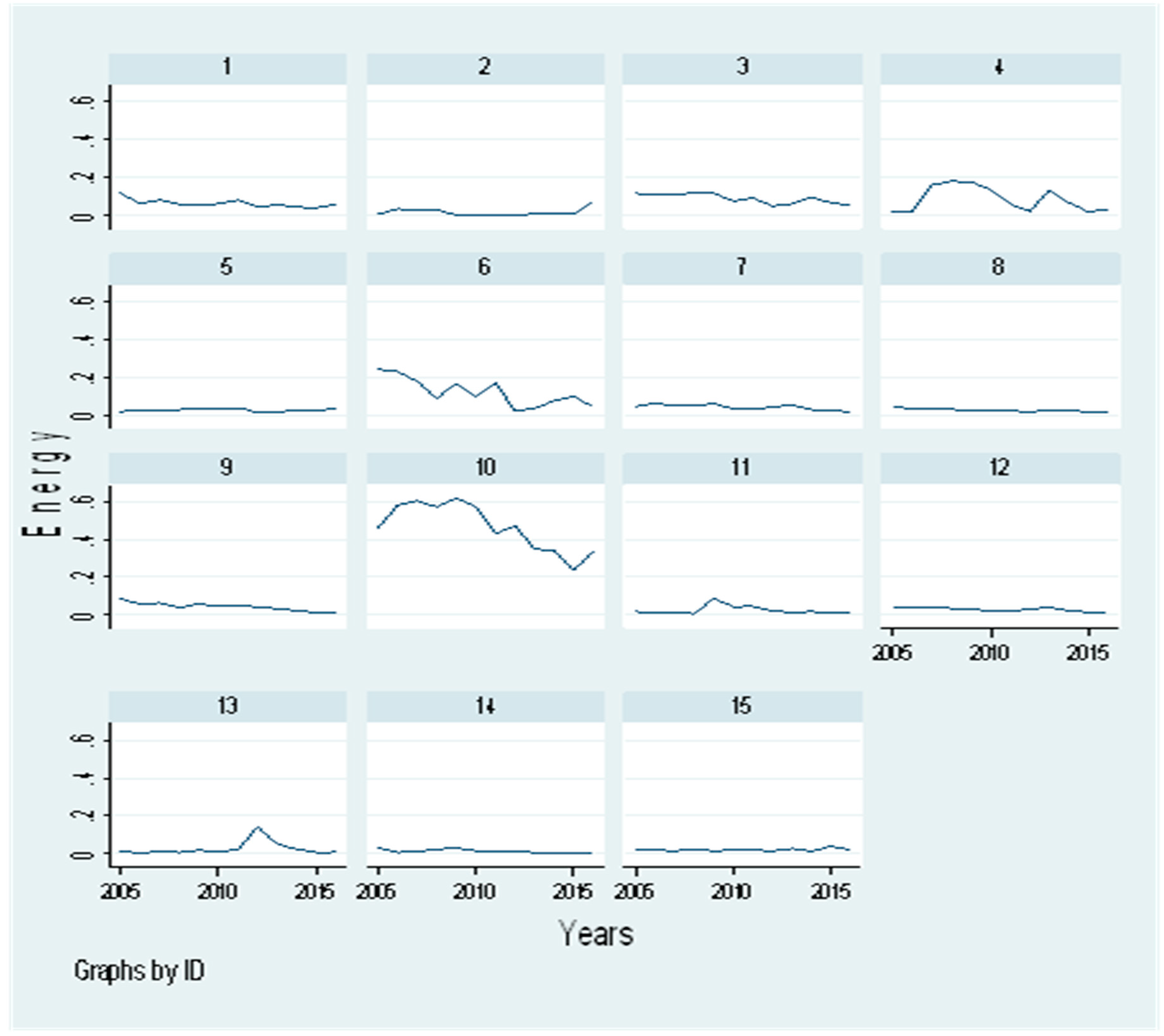
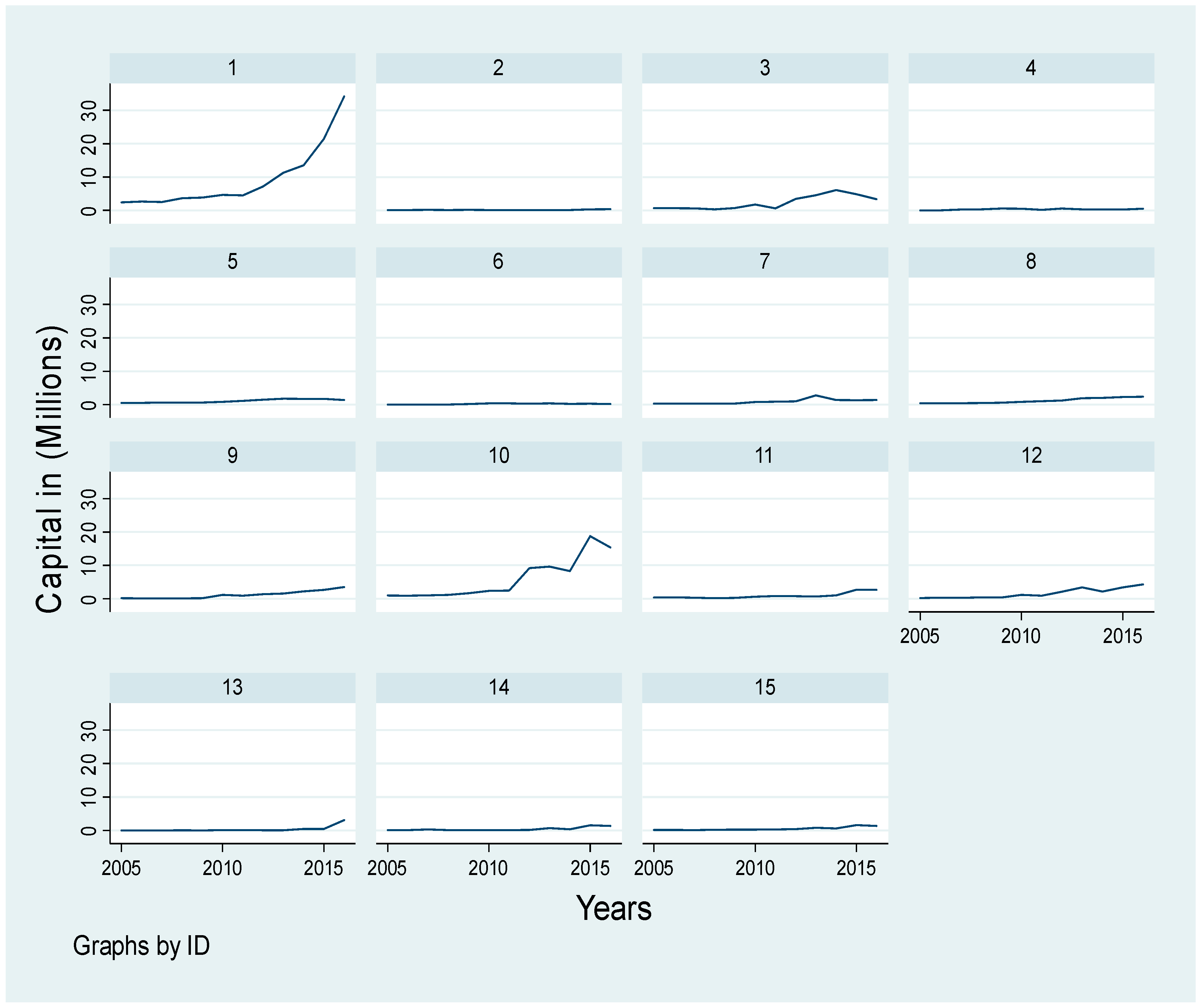
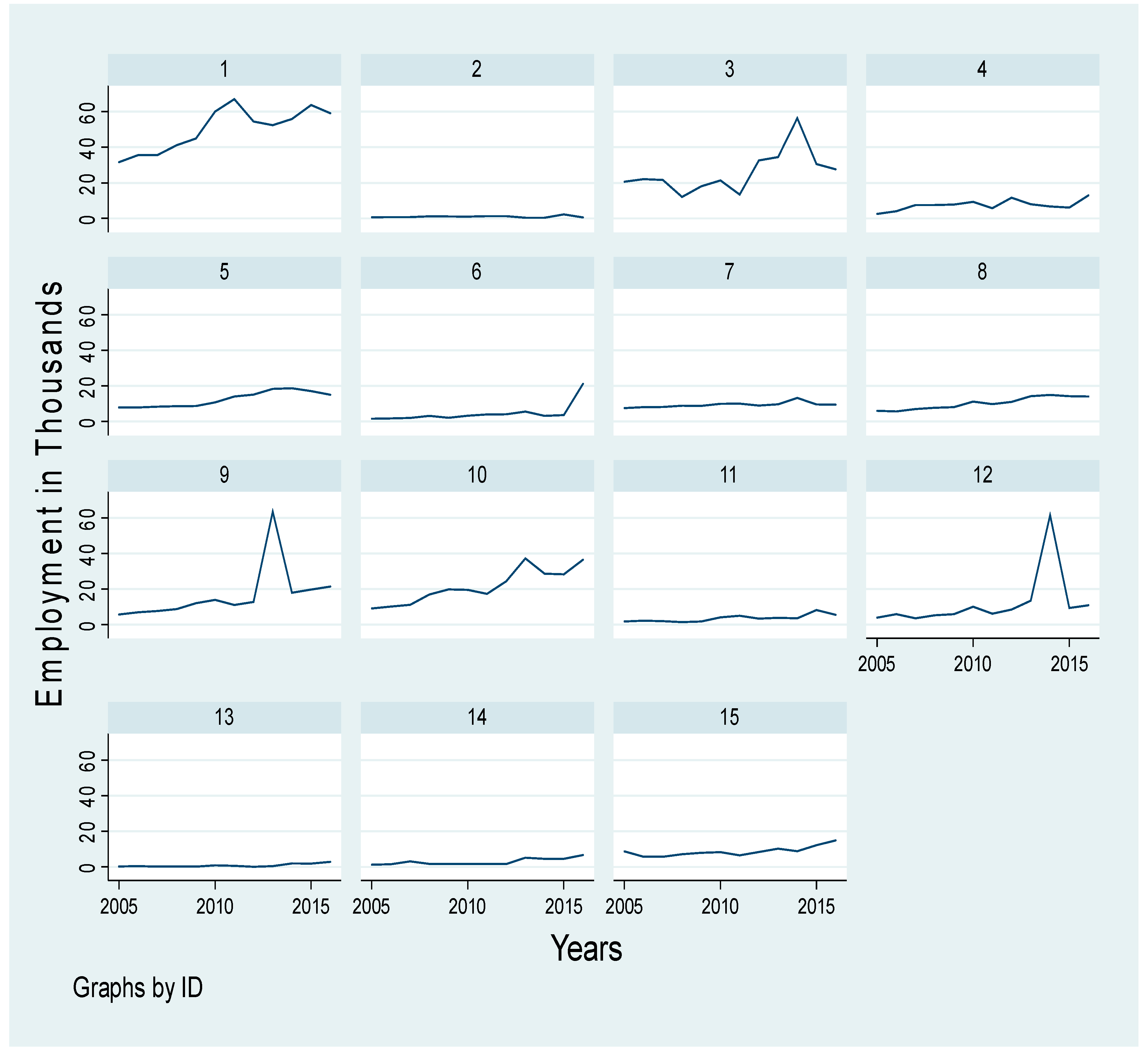
4.2. The Variables’ Development Over Time

Figure 1 gives the trends of production for the 15 industries included in this study. The industry classification is standard, as provided by the Statistics Authority of Ethiopia. A list of the 15 industry groups is reported in Table 1. Based on this, the food and beverage industry (industry code 1) shows an increasing trend for 10 years (2005–2016). Similarly, the other non-metallic mineral products industry (industry code 10) and the motor vehicle and trailer industry (industry code 14) show an increase in the recent years of the study period. However, the remaining industries have constant trends in production. Thus, the outcome of policies in the form of industrial development’s effects are heterogeneous across industry groups. Figure 2 presents the trends of energy use across the industry groups. With the exception of the wood products industry (industry code 6) and the non-metallic mineral industry (industry code 10), the overall trends in energy use throughout the decade, on average, show steady growth. However, these two industries are relatively more energy intensive and, very recently, a decline in energy use has been witnessed in both these industries.
Figure 3 and Figure 4 give the trends of capital and employment in the 15 industry groups in the study period. The use of capital increased over time for the food and beverage industry (industry code 1) and the non-metallic mineral products industry (industry code 10) compared to the other industry groups. Employment in the food and beverage industry (industry code 1) as well as the textile industry (industry code 3), on average, showed an upward trend throughout while the rubber and plastic industry (industry code 9) and the metallic industry (industry code 12) had huge employment in the second half of the study period but, overall, had a flatter upward trend over time. In the remaining industry groups, the overall employment trend was steady.
Figure 5 and Figure 6 show the share of production and energy use by the manufacturing industry groups. The food and beverage industry (code 1) had the lion’s share in terms of production followed by the non-metallic mineral products industry (code 10). The apparel industry (code 4), wood industry (code 6), and machinery industry (code 13) had the lowest shares compared to the other industry groups. The energy use share was the highest in the metallic industry (code 10), followed by the wood industry (code 6), the apparel industry (code 4), and the textile industry (code 3).

5. Empirical Results and Discussion

5.1. Descriptive Statistics

Table 3 gives the summary statistics of the variables of interest. It gives information about the overall, between, and within variations in terms of mean and standard deviations, together with the minimum and maximum values of the variables. The total sample is 180 observations: 15 industry groups and 12 years of data from 2005 to 2016. In the summary, we included variables such as industry production, employment, and labor productivity, defined as the ratio of production per employee in the industry groups, capital proxied by fixed assets, and the value of energy and human capital proxied by wages and salaries. Accordingly, for variables such as production per employee and the value of energy, the within variations are higher than the between variations, while the within variations of labor and capital are higher than the between variations. The minimum and maximum values of each variable are also given in Table 3.

5.2. Regression Results and Analysis

In this section, static and dynamic panel data models are estimated for the industry panel data available from 2005 to 2016. The data contains 15 industry groups listed in Table 1 and all of them are included in the analysis. Thus, the data includes the entire population of the industry groups. The estimated models are pooled OLS, fixed effects (FE), and random effects (RE) models from the static panel estimators, while difference GMM and system GMM are presented as dynamic estimators. Three different model specifications are used in the estimation. In the first model, industry group production is the dependent variable, while energy, labor, and capital are explanatory variables. In this model, the returns in relation to the scale of production are calculated based on the sum of the coefficients for the three input variables. In the second model, manufacturing labor productivity is specified as employment (labor), capital (fixed assets), value of energy, and time trend (technology) as the explanatory variables. In this model, the coefficients measure the scale effect of the explanatory variables on labor productivity of the industry groups and labor represents the scale effect. In the third model, the manufacturing sector’s labor productivity is explained by measuring energy and capital intensities respectively. In all the three model specifications, a trend is included to capture a shift in the labor productivity function or rate of technological change. All variables (with the exception of trend) are transformed into logarithmic form so that the coefficients are interpreted as input elasticities.
Accordingly, Table 4 shows the results of the pooled OLS for the three model specifications. In the first model, labor, capital, energy, and technology are found to be statistically significant and positive. These are among the key factors used for explaining the manufacturing industry’s production growth. The elasticity of the output with respect to capital is higher than the corresponding figures for labor and energy in these industries. The returns in relation to the scale of the production process are 1.06 implying increasing returns in relation to scale in this specification coinciding with predictions in the literature [1,67]. In the second model, labor is significant and positive at the one percent significance level. However, we do not interpret the coefficient of labor and, instead, based on Equation (5d), we find the value of α by adding one to the estimated coefficient in our model, which is zero. Then α, in our case, will be positive, indicating the positive effect of labor on productivity in the manufacturing industries. This can be attributed to the increasing returns in relation to the scale of production and the type of existing industries, which are dominated by labor-intensive industries. In this model, capital is significant and positive for labor productivity, which is a boost for the industry groups. These results are in accordance with Otalu and Anderu and Velucchi Viviani [7,43]. Energy use also positively effects productivity in line with other empirical studies [40,41,42,43,44,45]. In the third model, capital and energy intensities are significant and positive and help explain labor productivity in the manufacturing industries in line with other studies [46,50,51]. Our results confirm that labor productivity is high and more elastic for energy intensity than for capital in the Ethiopian manufacturing industries. The models show that adjusted R2 is high and the probability of F-statistics is significant, confirming the appropriateness of the model’s specifications (see Table 4).
It should be noted that the pooled OLS model ignores industry effects that may generate biased results. However, it serves well to establish the model’s specifications. Table 5 presents the static panel data model estimation results. In this section, only the second and third models are estimated using fixed effects (FE) and random effects (RE) estimation methods. The fixed effects model allows the industry effects and inputs to be correlated, while the random effects model assumes that these are not correlated. The fixed effects model is consistent and unbiased regardless of the correlated effects, but the random effects model is valid and efficient. In this case, since the industry groups are made up of the population of industries, the fixed effects model is a better choice. For a comparison, we estimate the models using both estimation methods.
In the fixed effects model, labor is statistically significant and is a positive factor in explaining the variations in manufacturing productivity in Ethiopia. This is expected based on theoretical predictions as more labor employment induces labor productivity. The fixed effects model’s estimation results confirm that energy, capital, and technology positively effects labor productivity, and all of them are statistically significant at the one percent level of significance. The input intensity model based on the fixed effects estimation shows that capital intensity and energy intensity are statistically significant factors for explaining labor productivity in the Ethiopian manufacturing industries. However, in this case, productivity is more elastic in relation to capital intensity than energy intensity. In the random effects model, energy, capital, and technology are positive and statistically significant in explaining the industry groups’ labor productivity, while the coefficient for labor is negative, but, based on Equation (5d), α is found by adding one to the coefficient, which gives us a positive coefficient with a value of 0.45. For the intensity model, the random effects estimation approach confirms the significance of energy and capital intensities positively effecting labor productivity. Like the fixed effects model’s results, productivity is less elastic in relation to energy intensity than it is to capital intensity. In all the models, the coefficients for trends are positive and significant, implying a positive shift in labor productivity because of technological changes in Ethiopian manufacturing industries during the study period.
The models give different results for some of the explanatory variables, so we cannot take into account the results of all the models. Instead, we must select a model that explains the data using different tests and base the analysis on the optimal model’s specifications. To choose between pooled and random effects models, we used the Breusch and Pagan lagrange multiplier (LM) tests with the null hypothesis that pooled OLS is an appropriate model that explains the data better relative to the random effects model. The Hausman test compares the random effects model with the fixed effects model and the null hypothesis for the Hausman test shows that the random effects model is not appropriate for representing the data relative to the fixed effects model. Accordingly, in both cases, the p-value of chi2 and chibar2 forces us to reject the null hypothesis. Therefore, the fixed effects model is preferred to the pooled OLS model and the fixed effects model is preferred to the random effects model to represent our data. To control for the heteroscedasticity problem, standard errors reported in all the models are robust.
Table 6 gives the dynamic panel model’s estimation results for both the difference GMM and system GMM models. Unlike static panel models, these models include the lag of the dependent variable as an explanatory variable in addition to the other variables. In the dynamic models, problems of heteroscedasticity and autocorrelation are considered. In both the scale effects (Model 2) and the input intensity models (Model 3), lagged labor productivity is found to be significant and positive in explaining changes in the manufacturing industry’s labor productivity in Ethiopia. This shows that the previous year’s productivity increases current productivity, which, in our case, is labor productivity. An increase in employment for the industry groups has a positive and significant effect which is attributed to increasing returns to scale and the labor-intensive nature of manufacturing industries in both the cases. In both the difference GMM and system GMM models, energy induces labor productivity. Comparing our results with those from developing countries suggests that our results are in line with those from some sub-Saharan African countries, such as those reported by Kebede et al. and Akinlo [12,18]. However, the effect of energy on productivity for some African countries shows that it is not as important as labor and capital [10,39], signifying the mixed empirical results of the relationship between energy and growth as one major reason for undertaking this specific study. The empirical validation in our case is at the industry level and not at the aggregate national level and this is one of the contributions of this study to the existing literature, as it is what makes this study different from the existing studies. Unlike other studies, the consistency of our results is empirically confirmed using different model specifications and alternative estimation strategies. In addition to the role of energy in productivity, the effects of labor, capital, and technological change on manufacturing productivity are also empirically validated in Ethiopia. This provides crucial policy input for the country’s industrial policy.
In the input intensity model (Model 3), the elasticity productivity for energy intensity is higher than capital intensity, while the opposite is the case for the system GMM model. Capital is positive and significant in all the models for increasing labor productivity. The coefficient of the time trend has a positive sign in all the models, indicating technological progress with an expected positive effect on the productivity of the industries (see Table 6).
Table 7 discusses the results of the system GMM dynamic estimator, including dummies for trends. Our results show that, in both the models, energy magnitude and energy intensity are statistically significant and positive factors in increasing labor productivity in the manufacturing industry groups; this finding coincides with other findings in the literature [34,35,36]. Besides, the magnitude of capital and capital intensity are positive factors for labor productivity. In both the models, time dummies are positive throughout. The results show that there is no cyclical effect and, instead, labor productivity increases in both cases over time, which can be attributed to technical changes, increasing labor productivity.
One major objective of this study was to ascertain whether an empirical relationship existed between energy and labor productivity in Ethiopian industries, along with investigating whether it positively affected productivity or limited it. The results of all the models confirm that the energy-related parameter is significant and positive, showing that an increase in energy consumption enhances labor productivity in Ethiopian manufacturing industry groups. This result coincides with other empirical studies [15,16,17,46]. However, in Ethiopia, agriculture was previously a major source of livelihood for the population. Agriculture was a dominant sector in terms of the employment share up until recently, when traditional services emerged to dominate the economy [21,23]. The share of manufacturing in Ethiopian GDP was very low, indicating output and premature deindustrialization [20,21,24]. This requires serious engagement for identifying and prioritizing the major explanatory factors for the manufacturing industry. Furthermore, manufacturing is more energy intensive relative to other sectors and the interdependence between energy and industries is a crucial tool for sustainable economic development [6,32]. Accordingly, empirically identifying the role of energy in the manufacturing productivity of Ethiopia can contribute to industrial policy input. The labor input is significant and positive in the scale effects model (Model 2). This means that an increase in labor employment will increase labor productivity due to increasing returns and the labor-intensive nature of the industries [7,30]. Finally, we reported the diagnostic tests for serial correlation and heteroscedasticity. The AR (2) test validated the model, free from the serial correlation problem. The number of instruments used were less than the groups in both the dynamic panel estimation approaches.

6. Conclusions and Policy Implications

This study investigated the effect of energy on manufacturing labor productivity in Ethiopia using panel data for manufacturing industry groups. Fifteen industries were included in the study covering 12 years of data from 2005 to 2016. The number of industry groups and the period was determined by data availability. Data were obtained from the Central Statistical Authority (CSA) in Ethiopia. We used both descriptive and econometric approaches for examining the empirical relationships between the variables of interest conditional on some other variables and characteristics. This study had two specific objectives: examining the existence of an empirical relationship between energy and labor productivity in the manufacturing industry and estimating the elasticity effect of energy on labor productivity.
Three models were estimated. The first model is a conventional production function with labor, capital, and energy as the explanatory variables along with a time trend to proxy for capturing technological change. The second model measures the scale effect of energy with the control variables labor, capital, and technology. The third model measures the intensity effect of energy and capital on labor productivity in Ethiopian manufacturing industries. Accordingly, static and dynamic panel data models were estimated—pooled OLS, fixed effects, and random effects static panel estimators, along with difference and system GMM dynamic panel models.
The data for industrial group production showed that the overall trends in production were steady and constant over the study period, except for the food and beverage industry, which rapidly increased (industry code 1). On average, the energy use trend increased in the food and beverage industry (industry code 1) as well as the textile industry (industry code 3). The share of production across the 15 industry groups was dominated by the food and beverage industry (industry code 1), followed by the non-metallic mineral products industry (industry code 10). The non-metallic mineral products industry was found to be more energy intensive than the others.
In the first model, the manufacturing production function was estimated with labor, capital, and energy as the inputs in the production process. The time trend was included to capture technological change. In this model, energy, capital, and labor were statically significant and positive in augmenting manufacturing production in Ethiopia; this result is similar to that of other empirical studies [15,16,17]. Technology was also significant and a positive factor in industrial growth in Ethiopia. In this model, the sample average returns in relation to the scale of production were 1.07, implying increasing returns in relation to the scale of the manufacturing industries. Labor and capital were statistically significant in all the models at the one percent level of significance.
Across the models, some variables had different significance levels, which led us to select an appropriate model that fit the data best. Both static and dynamic model estimation methods were considered, and we got different estimated coefficient results. For the static models, limitations in considering endogeneity, omitted variable bias, autocorrelation, and heteroscedasticity led to the dynamic panel model estimator being selected over the static panel estimator. The system GMM estimator was chosen over the difference GMM model based on the diagnostic tests and to overcome the limitations of missing observations in the difference GMM model.
In all the models, an increase in employment induced labor productivity due to increasing returns to scale and the labor-intensive nature of the industries. Energy positively explains labor productivity in manufacturing industries in Ethiopia. This means an increase in the use of energy-enhanced labor productivity in the industry groups. Capital intensity use gave a boost to labor productivity, which is consistent with theoretical predictions. In addition, a system GMM model was estimated, including time dummies for the scale effect and input intensity models. In both the cases, labor productivity increased over time, signifying the positive effect of technical change on manufacturing labor productivity in Ethiopia. Across the different approaches used, the role of energy use and energy intensity was consistently significant and positive in explaining labor productivity changes in Ethiopian manufacturing industries.
This study showed that energy induces labor productivity in the manufacturing industry groups in Ethiopia, showing that the efficient use of energy increases industrial growth. It also empirically identified labor and capital as essential determinant factors of productivity in the manufacturing industries in Ethiopia, complemented by technological change effects. This indicates a need to organize resources in a way that boosts the growth of the industries. Energy and capital should also be efficiently used, as the results show that productivity is elastic in relation to a change in energy and capital input intensities in the manufacturing industries in Ethiopia.
A review of the existing literature showed that the role of energy in productivity is controversial across countries [10,17,44,57]. This study adds to the literature by empirically validating the positive role of energy in productivity, applying different model specifications and estimation methods to Ethiopia’s manufacturing industries. This implies that industrial policies in Ethiopia should focus on the efficient use of energy along with labor, capital, and technical changes to overcome the premature deindustrialization pattern over time. Research on the energy efficiency and energy productivity of the manufacturing industries in Ethiopia is expected to provide additional policy inputs. This type of research can be extended to cross-country analyses in developing countries, using the manufacturing industry as a case study.

Author Contributions

Conceptualization, S.G.K. and A.H.; methodology, S.G.K. and A.H.; Data collection, S.G.K.; Formal analysis, S.G.K.; writing—original draft preparation, S.G.K. and A.H.; writing—review and editing, S.G.K. and A.H. All authors have read and agreed to the published version of the manuscript.

Funding

This research received no external funding.

Acknowledgments

The authors gratefully acknowledge the comments and suggestions by the editor of the journal and three anonymous referees on an earlier version of this manuscript.

Conflicts of Interest

The authors declare no conflict of interest.

References

  1. Kaldor, N. Causes of the Slow Rate of Economic Growth of the United Kingdom. An Inaugural Lecture; Cambridge University Press: Cambridge, UK, 1966. [Google Scholar]
  2. Cornwall, J. Modern Capitalism. Its Growth and Transformation; St. Martin’s Press: New York, NY, USA, 1977. [Google Scholar]
  3. Guadagno, F. The determinants of Industrialization in Developing Countries, 1960–2005. UNU-MERIT Maastricht Univ. 2016, 31, 26. [Google Scholar]
  4. UNECA. Dynamic Industrial Policy in Africa: Economic Report on Africa; UNECA: Addis Ababa, Ethiopia, 2014. [Google Scholar]
  5. UNECA. Industrializing Through Trade. Economic Report on Africa; UNECA: Addis Ababa, Ethiopia, 2015. [Google Scholar]
  6. UNIDO. Demand for Manufacturing: Driving Inclusive and Sustainable Industrial Development. Industrial Development Report; United Nations Industrial Development Organization UNIDO: Vienna, Austria, 2018. [Google Scholar]
  7. Otalu, J.A.; Anderu, K.S. An Assessment of the Determinants of Industrial Sector Growth in Nigeria. J. Res. Bus Man 2015, 3, 1–9. [Google Scholar]
  8. Story, D. Time-Series Analysis of Industrial Growth in Latin America: Political and Economic Factors. Soc. Sci. Quart. 1980, 61, 293–307. [Google Scholar]
  9. UNDP (United Nations Development Program). Transforming Lives Through Renewable Energy Access in Africa UNDP’s Contributions. UNDP Afr. Policy Brief 2018, 1, 1–26. [Google Scholar]
  10. Chen, P.Y.; Chen, S.T.; Chen, C.C. Energy consumption and economic growth—New evidence from meta-analysis. Energy Policy 2012, 44, 245–255. [Google Scholar] [CrossRef]
  11. Moghaddasi, R.; Pour, A.A. Energy Consumption and Total Factor productivity in Iranian Agriculture. Energy Rep. 2016, 2, 218–220. [Google Scholar] [CrossRef] [Green Version]
  12. Kebede, E.; Kagochi, J.; Jolly, C.M. Energy consumption and economic development in Sub-Sahara Africa. Energy Econ. 2010, 32, 532–537. [Google Scholar]
  13. Al-Iriani, M.A. Energy-GDP relationship revisited: An Example from GCC Countries Using Panel Causality. Energy Policy 2005, 34, 3342–3350. [Google Scholar] [CrossRef]
  14. Cleveland, C.J.; Kaufmann, R.K.; Stern, D.I. Aggregation and the role of energy in the economy. Ecol. Econ. 2000, 32, 301–317. [Google Scholar] [CrossRef]
  15. Alaali, F.; Roberts, J.; Taylor, K. The Effect of Energy Consumption and Human Capital on Economic Growth: An Exploration of Oil Exporting and Developed Countries. SERPS (Sheffield Econ. Res. Pap. Ser.) 2015, 2015015. [Google Scholar]
  16. Fallahi, F.; Sojood, S.; Aslaninia, N.M. Determinants of Labor Productivity in Iran’s Manufacturing Firms: With Emphasis on Labor Education and Training. MPRA 2010, 27447. [Google Scholar]
  17. Soytas, U.; Sari, R. Energy consumption and GDP: Causality relationship in G-7 countries and emerging markets. Energy Econ. 2003, 25, 33–37. [Google Scholar] [CrossRef]
  18. Akinlo, A.E. Energy consumption and economic growth: Evidence from 11 Sub-Sahara African countries. Energy Econ. 2008, 30, 2391–2400. [Google Scholar] [CrossRef]
  19. CSA (Central Statistic Authority). Industry Sector Data Base of Ethiopian Industries; CSA: Addis Ababa, Ethiopia, 2018. [Google Scholar]
  20. EEA (Ethiopian Economic Association). Data Base on Macroeconomic Variables; EEA: Addis Ababa, Ethiopia, 2017. [Google Scholar]
  21. Ejigu, Z.K.; Singh, I.S. Service Sector: The Source of Output and Employment Growth in Ethiopia. Acad. J Econ. 2016, 2, 139–156. [Google Scholar]
  22. Oqubay, A. Industrial Policy and Late Industrialization in Ethiopia; Working paper Series No. 303; African Development Bank: Abidjan, Cote D’Ivoire, 2018. [Google Scholar]
  23. Gebreeyesus, M. Industrial Policy and Development in Ethiopia: Evolution and Present Experimentation; UNU.WIDER Working Paper No 6; UNU.WIDER: Helsinki, Finland, 2010. [Google Scholar]
  24. Rodrik, D. Premature deindustrialization. J Econ. Growth 2016, 21, 1–33. [Google Scholar] [CrossRef]
  25. Ray, D. Development Economics; Princeton University Press: Princeton, NJ, USA, 1998. [Google Scholar]
  26. Romer, D. Advanced Macroeconomics, 4th ed.; University of California: Berkeley, CA, USA, 2011. [Google Scholar]
  27. Todaro, M.P.; Smith, S.C. Economic Development, 12th ed.; Pearson Education Inc.: New Jersey, USA, 2015. [Google Scholar]
  28. Agénor, P.R.; Montiel, P. Development Macroeconomics, 3rd ed.; Princeton University Press: Princeton, NJ, USA, 2008. [Google Scholar]
  29. Stern, D.I. The Role of Energy in Economic Growth CCEP; Working Paper 3.10; Crawford School, The Australian National University: Canberra, Australia, 2010. [Google Scholar]
  30. Su, B.; Heshmati, A. Development and Sources of Labor Productivity in Chinese Provinces. China Econ. Policy Rev. 2014, 2, 1–30. [Google Scholar]
  31. Stern, D.I. Limits to Substitution and Irreversibility in Production and Consumption: A Neoclassical Interpretation of Ecological Economics. Ecol. Econ. 1997, 21, 197–215. [Google Scholar] [CrossRef]
  32. OECD. Energy; OECD Green Growth Studies; OECD Publishing: Paris, France, 2012. [Google Scholar]
  33. UNDP (United Nations Development Program). Energy for Sustainable Development a Policy Agenda; UNDP: New York, NY, USA, 2002. [Google Scholar]
  34. Toman, M.A.; Jemelkova, B. Energy and economic development: An assessment of the state of knowledge. Energy J. 2003, 24, 93. [Google Scholar] [CrossRef]
  35. Cabraal, R.A.; Barnes, D.F.; Agarwal, S.G. Productive Uses of Energy for Rural Development. Ann. Rev. Environ. Res. 2005, 30, 117–144. [Google Scholar] [CrossRef]
  36. Ejaz, Z.; Aman, M.U.; Usman, M.K. Determinants of Industrial Growth in South Asia: Evidence from Panel Analysis. In Papers and Proceedings; Unpublished; 2016; pp. 97–110. Available online: https://www.pide.org.pk/psde/pdf/AGM33/papers/M%20Aman%20Ullah.pdf (accessed on 26 May 2020).
  37. Heshmati, A. Productivity Growth, Efficiency and Outsourcing in Manufacturing and Service Industries. J. Econ. Sur. 2003, 17, 79–112. [Google Scholar] [CrossRef]
  38. Rybár, R.; Kudelas, D.; Beer, M. Selected Problems of Classification of Energy Sources: What are Renewable Energy Sources? Acta Montan. Slovaca 2015, 20, 172–180. [Google Scholar]
  39. Wolde-Rufael, Y. Energy consumption and economic growth: The experience of African countries revisited. Energy Econ. 2009, 31, 217–224. [Google Scholar] [CrossRef]
  40. Schurr, S.H.; Netschert, B.C.; Eliasberg, V.E.; Lerner, J.; Landsberg, H.H. Energy in the American Economy; Johns Hopkins University Press: Baltimore, MD, USA, 1960. [Google Scholar]
  41. Schurr, S.H. Energy use, technological change, and productive efficiency: An economic-historical interpretation. Ann. Rev. Energy 1984, 9, 409–425. [Google Scholar] [CrossRef]
  42. Jorgenson, D.W. The role of energy in productivity growth. Energy J. 1984, 5, 26–30. [Google Scholar] [CrossRef]
  43. Boudreaux, B.C. The impact of electric power on productivity: A study of US manufacturing 1950–1984. Energy Econ. 1995, 17, 231–236. [Google Scholar] [CrossRef]
  44. Murillo-Zamorano, L.R. The role of energy in productivity growth: A controversial issue? Energy J. 2005, 26, 69–88. [Google Scholar] [CrossRef]
  45. Walheer, B. Labour productivity growth and energy in Europe: A production-frontier approach. Energy 2018, 152, 129–143. [Google Scholar] [CrossRef]
  46. Mahadevan, R.; Asafu-Adjaye, J. Energy consumption, economic growth and prices: A reassessment using panel VECM for developed and developing countries. Energy Policy 2007, 35, 2481–2490. [Google Scholar] [CrossRef]
  47. Velucchi, M.; Viviani, A. Determinants of the Italian Labor Productivity: A Quantile Regression Approach. Statistica 2011, 71, 213–238. [Google Scholar]
  48. Islam, S.; Shazali, S.S. Determinants of Manufacturing Productivity: Pilot Study on Labor-Intensive Industries. Int. J. Product. Perform. Manag. 2010, 60, 567–582. [Google Scholar] [CrossRef]
  49. Heshmati, A.; Rashidghalam, M. Labour productivity in Kenyan manufacturing and service industries. In Determinants of Economic Growth in Africa; IZA: Bonn, Germany, 2016. [Google Scholar]
  50. Nagler, P.; Naudé, W. Labor Productivity in Rural African Enterprises: Empirical Evidence from the LSMS-ISA; IZA Discussion Papers 8524; Institute of Labor Economics (IZA): Bonn, Germany, 2014. [Google Scholar]
  51. Samuel, B.; Aram, B. The Determinants of Industrialization: Empirical Evidence for Africa. Eur. Sci. J. 2016, 12, 219–239. [Google Scholar]
  52. OECD. Productivity Measurement and Analysis. Proceedings from OECD Workshops; Swiss Federal Statistical Office (FSO): Neuchâtel, Switzerland, 2008. [Google Scholar]
  53. OECD. Measuring Productivity—OECD Manual: Measurement of Aggregate and Industry-Level Productivity Growth; OECD Publishing: Paris, France, 2001. [Google Scholar]
  54. Hajkova, D.; Hurnik, J. Cobb-Douglas production function: The case of a converging economy. Czech J. Econ. Financ. 2007, 57, 465–476. [Google Scholar]
  55. Van Beven, L. Total Factor Productivity: A Practical View. J. Econ. Surv. 2010, 26, 98–128. [Google Scholar] [CrossRef] [Green Version]
  56. Del Gatto, M.; Di Liberto, A.; Petraglia, C. Measuring productivity. J. Econ. Surv. 2011, 25, 952–1008. [Google Scholar] [CrossRef]
  57. Cobb, C.W.; Douglas, P.H. A theory of production. Am. Econ. Rev. 1928, 18, 139–165. [Google Scholar]
  58. Murthy, K.V. Arguing a case for Cobb-Douglas production function. Rev. Commer. Stud. 2002, 20, 21. [Google Scholar]
  59. Zellner, A.; Kmenta, J.; Dreze, J. Specification and estimation of Cobb-Douglas production function models. Econom. J. Econom. Soc. 1966, 34, 784–795. [Google Scholar] [CrossRef]
  60. Eldridge, L.P.; Price, J. Measuring quarterly labor productivity by industry. Mon. Labor Rev. 2016, 139, 1–27. [Google Scholar] [CrossRef] [Green Version]
  61. Faustino, H.C.; Leitão, N.C. Intra-industry trade: A static and dynamic panel data analysis. Int. Adv. Econ. Res. 2007, 13, 313–333. [Google Scholar] [CrossRef]
  62. Hummels, D.; Levinsohn, J. Monopolistic competition and international trade: Reconsidering the evidence. Q. J. Econ. 1995, 110, 799–836. [Google Scholar] [CrossRef]
  63. Zhang, J.; van Witteloostuijn, A.; Zhou, C. Chinese bilateral intra-industry trade: A panel data study for 50 countries in the 1992–2001 period. Rev. World Econ. 2005, 141, 510–540. [Google Scholar] [CrossRef]
  64. Arellano, M.; Bond, S. Some Tests of Specification for panel data: Monte Carlo Evidence and an Application to Employment Equations. Rev. Econ. Stud. 1991, 58, 277–297. [Google Scholar] [CrossRef] [Green Version]
  65. Arellano, M.; Bover, O. Another look at the Instrumental Variable Estimation of Error-components Model. J. Econ. 1995, 68, 29–51. [Google Scholar] [CrossRef] [Green Version]
  66. Roodman, D. How to do xtbond2: An Introduction to Difference and System GMM in Stata. Stata J. 2009, 9, 86–136. [Google Scholar] [CrossRef] [Green Version]
  67. Rodrik, D. Unconditional Convergence in Manufacturing. Q. J. Econ. 2013, 128, 165–204. [Google Scholar] [CrossRef]
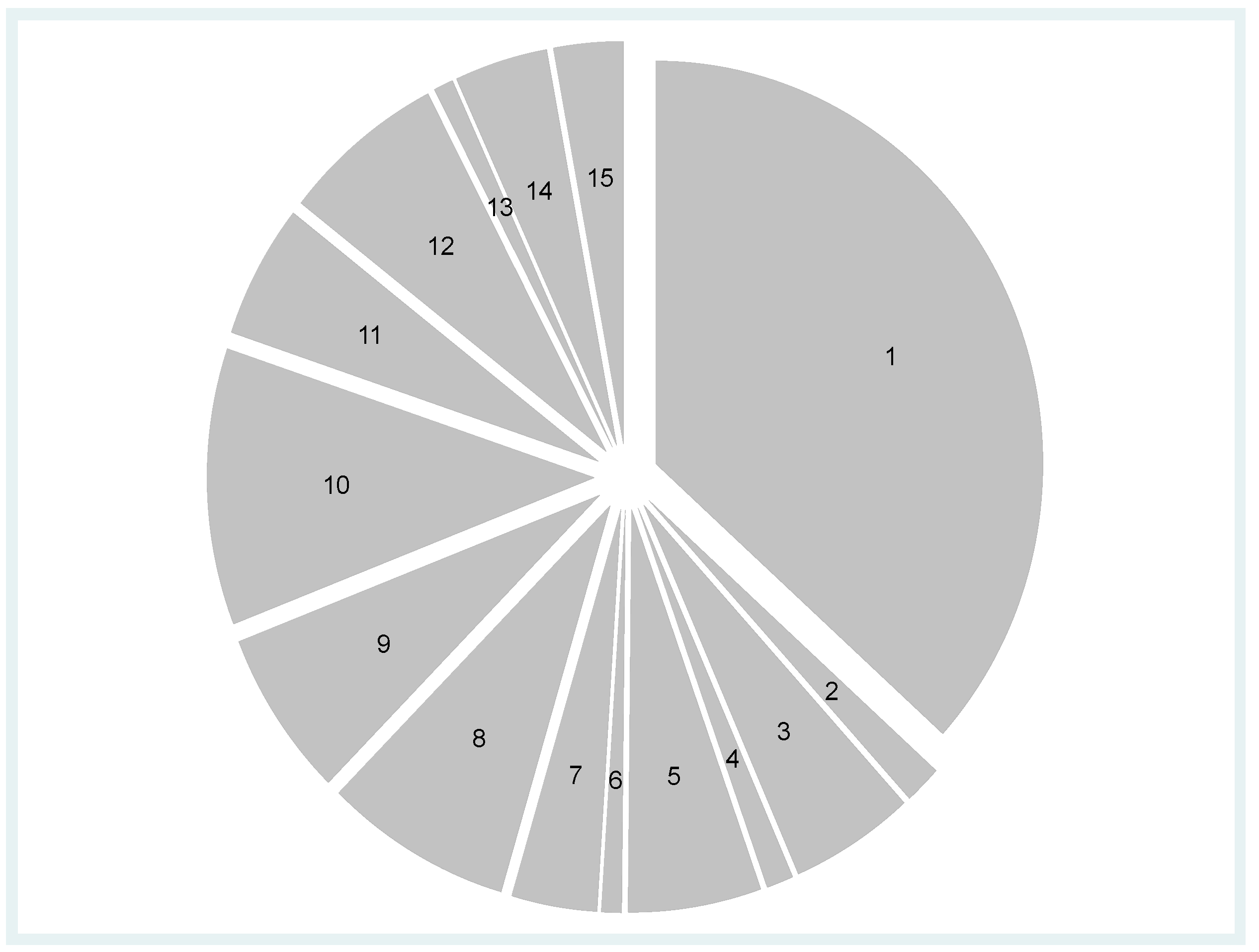
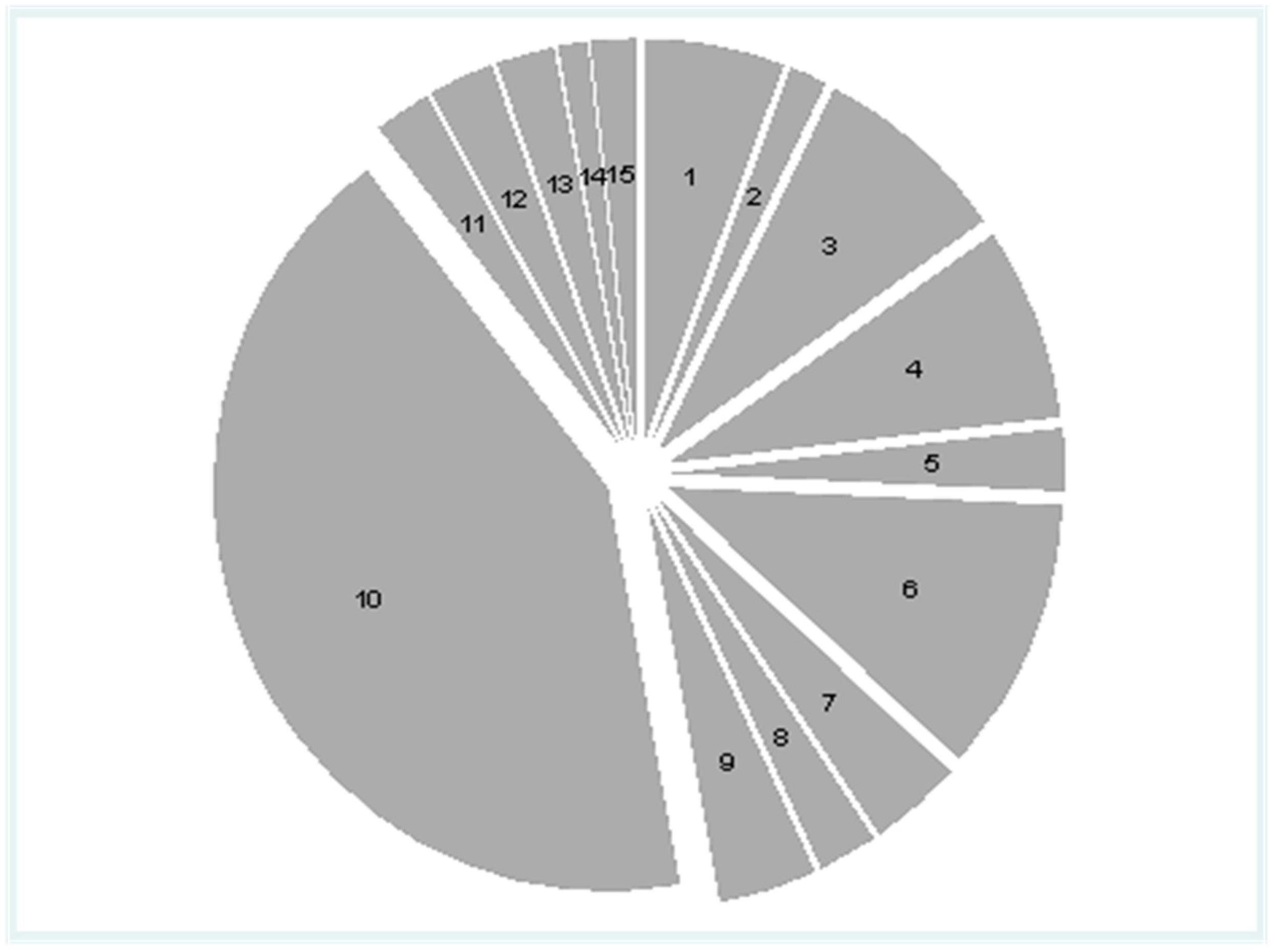
Figure 1. Production trends by industry groups.
Energies 13 02714 g001
Figure 2. Energy use trends by industry groups.
Energies 13 02714 g002
Figure 3. Capital trend by industry groups.
Energies 13 02714 g003
Figure 4. Employment trends by industry groups.
Energies 13 02714 g004
Figure 5. Gross value of production by industry groups.
Energies 13 02714 g005
Figure 6. Energy use across industry groups.
Energies 13 02714 g006
Table 1. List of industry groups.
Industry CodeIndustry Group (Sector)
1Food Products and Beverages Industry
2Tobacco Products Industry
3Textiles Industry
4Wearing Apparel, Except Fur Apparel Industry
5Tanning and Dressing of Leather; Footwear, Luggage, and Handbags Industry
6Wood and of Products of Wood and Cork, Except Furniture Industry
7Paper, Paper Products, and Printing Industry
8Chemicals and Chemical Products Industry
9Rubber and Plastic Products Industry
10Other Non-Metallic Mineral Products Industry
11Basic Iron and Steel Industry
12Fabricated Metal Products Except Machinery and Equipment Industry
13Machinery and Equipment Industry
14Motor Vehicles, Trailers and Semi-Trailer Industry
15Furniture; Manufacturing Industry
Source: Central Statistical Authority (CSA).
Table 2. List of variables, expected level of significance, and coefficient signs.
VariablesVariable DefinitionsExpected Effect
Dependent variable:
Labor ProductivityRatio of gross value of production to number of employees-
Independent variables:
ProductionGross value of production by industrial group (in 000 Birr)-
EmploymentNumber of employees by industrial grouppositive
EnergyRatio of value of energy consumed to total industrial expenditure by industry grouppositive
CapitalTotal value of fixed assets by industry group (in 000 Birr)positive
Time trendIs a proxy for technical change and is included in the model as a control variablepositive
Table 3. Summary statistics of the variables of interest.
VariableVariationsMeanStd. Dev.MinimumMaximumObservations
IDOverall84.3349115NT = 180
Between 4.4721115N = 15
Within 088T = 12
YearsOverall2010.53.461620052016NT = 180
Between 02010.52010.5N = 15
Within 3.461720072016T = 12
ProductionOverall453,2408,002,421136735.54 × 107NT =180
Between 5,985,648551,875.12.50 × 107N = 15
Within 5,514,752−1.60 × 1073.50 × 107T = 12
EmploymentOverall12,512.614,497.454867,072NT = 180
Between 12,699.8681350,190.67N = 15
Within 7668.181−5985.01162,091.91T = 12
ProductivityOverall428.838563.594719.64284078.363NT = 180
Between 364.350585.99311470.145N = 15
Within 439.3695−587.82833037.057T = 12
Capital Overall175,3293,860,28146863.42 × 107NT = 180
Between 2,541,552160,494.19,332,244N = 15
Within 2973086−5,173,3602.66 × 107T = 12
EnergyOverall0.07300.117740.00100.6210NT = 180
Between 0.112850.01320.4650N = 15
Within 0.04369−0.15390.2290T = 12
Cost of LaborOverall275,439488,709.713294,023,882NT = 180
Between 351,034.530,176.831,466,912N = 15
Within 350,976.4−867,7612,832,410T = 12
Source: Authors’ computations using Stata.
Table 4. Pooled OLS estimation results for the three models.
VariablesModel 1Model 2Model 3
Robust Robust Robust
Coef.Std. ErrCoef.Std. ErrCoef.Std. Err
Labor (log)0.2730 ***(0.0755)−0.7269 ***(0.0755)--
Capital (log)0.7029 ***(0.0544)0.7027 ***(0.0544)0.0014 ***0.0004
Energy (log)0.0895 ***(0.0146)0.0895 ***(0.0146)0.1082 ***0.0127
Time trend0.0226 ***(0.0502)0.0226 ***(0.0050)0.0374 ***0.0088
Constant0.7930 ***(0.1996)0.7930 ***(0.1996)1.7272 ***0.0541
RTS1.0655
AdjR20.8979 0.8285 0.6074
F-statistics (p-value)0.0000 0.0000 0.0000
Notes: ***, **, * denote the statistical significance levels at 1%, 5%, and 10%, respectively. *Model 1: Output is the dependent variable. *Model 2: Labor productivity is the dependent variable (scale effect). *Model 3: Labor productivity is the dependent variable (input intensity effect).
Table 5. Static panel estimation results for Models 2 and 3.
Fixed EffectsRandom Effects
VariablesModel 2Model 3Model 2Model 3
Coef.Coef.Coef.Coef.
Log Labor−0.5541 ***
(0.1287)
-
-
−0.5748 ***
(0.1311)
-
-
Log Capital0.3545 ***
(0.0420)
0.3807 ***
(0.0475)
0.4205 ***
(0.0449)
0.4513 ***
(0.0562)
Log Energy0.0405 **
(0.0209)
0.0335 ***
(0.0113)
0.0474 ***
(0.0201)
0.0487 ***
(0.0182)
Time Trend0.0552 ***
(0.0075)
0.0454 ***
(0.0045)
0.0486 ***
(0.0065)
0.0400 ***
(0.0046)
Constant2.0353 ***
(0.5567)
1.3045 ***
(0.0822)
1.7624 ***
(0.4978)
1.1679 ***
(0.1056)
TestH0 & H1Appropriate ModelProb of chi2 & chibar2Decision
Breusch and Pagan LM TestH0Pooled OLS0.000reject H0
H1Random Effects
Hausman testH0Random Effects0.000reject H0
H1Fixed Effects
Notes: ***, **, * denote statistical significance levels at the 1%, 5%, and 10%, respectively. *Model 2: Labor productivity as the dependent variable (scale effect). *Model 3: Labor productivity as the dependent variable (intensity effect).
Table 6. Dynamic panel estimation results for Models 2 and 3.
Difference GMMSystem GMM
VariablesModel 2Model 3Model 2Model 3
Coef.Coef.Coef.Coef.
Productivity_L10.1443
(0.1286)
0.1210
(0.1667)
0.1342 **
(0.0592)
0.0990
(0.1004)
Log Labor−0.6557 ***
(0.1155)
-
-
−0.5997 ***
(0.0549)
-
-
Log Capital0.5438 ***
(0.0516)
0.0007 ***
(0.0002)
0.5276 ***
(0.0442)
0.5391 ***
(0.0373)
Log Energy0.0393 ***
(0.0188)
0.0221
(0.0153)
0.0357 ***
(0.0098)
0.0311 ***
(0.0071)
Time trend0.0263 ***
(0.0091)
0.0451 ***
(0.0157)
0.0255 ***
(0.0039)
0.0251 ***
(0.0086)
Constant1.1946 ***
(0.4445)
1.6935 ***
(0.3551)
1.0919 ***
(0.2333)
0.8973 ***
(0.2006)
AR (2) 0.4990.520
Test for autocorrelation 0.19580.1287
Number of instruments 54
Number of groups 1515
Notes: ***, **, * denote the statistical significance levels at 1%, 5%, and 10% levels respectively. *Model 2: Labor productivity as the dependent variable (scale effect) *Model 3: Labor productivity as the dependent variable (input intensity effect).
Table 7. System GMM dynamic panel with time dummies for Models 2 and 3.
System GMM Dynamic Panel (With Time Dummies)
Scale Effect Model
(Model 2)
Input Intensity Effect Model
(Model 3)
Coff.Std. ErrCoff.Std. Err
Productivity_L10.1653 *(0.0877)0.1660 *(0.0874)
Log Labor−0.6872 ***(0.0607)--
Log Capital0.6784 ***(0.0545)0.7145 ***(0.0481)
Log Energy0.0954 ***(0.0171)0.0947 ***(0.0108)
D.trend(2)0.7977 ***(0.1921)0.0709(0.0805)
D.trend(3)0.8422 ***(0.1929)0.1068 **(0.0805)
D.trend(4)0.8978 ***(0.1933)0.1632(0.0805)
D.trend(5)0.8448 ***(0.1982)0.1036(0.0807)
D.trend(6)0.8115 ***(0.2085)0.0744(0.0817)
D.trend(7)0.9268 ***(0.2058)0.1885 **(0.0814)
D.trend(8)0.9867 ***(0.2121)0.2669 ***(0.0832)
D.trend(9)1.0325 ***(0.2178)0.2701 ***(0.0835)
D.trend(10)1.0505 ***(0.2191)0.2948 ***(0.0832)
D.trend(11)0.9460 ***(0.2271)0.1892 **(0.0858)
D.trend(12)0.9808 ***(0.2277)0.2142 **(0.0857)
AR (2)0.853 0.779
Test for Autocorrelation0.1200 0.1287
Number of Instruments14 14
Number of groups15 15
Notes: ***, **, * denote the statistical significance levels at 1%, 5%, and 10% levels respectively. *Model 2: Labor productivity as the dependent variable (scale effect). *Model 3: Labor productivity as the dependent variable (input intensity effect).

