Frequency-Domain Nonlinear Modeling Approaches for Power Systems Components—A Comparison

Abstract

Harmonic simulations play a key role in studying and predicting the impact of nonlinear devices on the power quality level of distribution grids. A frequency-domain approach allows higher computational efficiency, which has key importance as long as complex networks have to be studied. However, this requires proper frequency-domain behavioral models able to represent the nonlinear voltage–current relationship characterizing these devices. The Frequency Transfer Matrix (FTM) method is one of the most widespread frequency domain modeling approaches for power system applications. However, others suitable techniques have been developed in the last years, in particular the X-parameters approach, which comes from radiofrequency and microwave applications, and the simplified Volterra models under quasi-sinusoidal conditions, that have been specifically tailored for power system devices. In this paper FTM, X-parameters and simplified Volterra approaches are compared in representing the nonlinear voltage –current relationship of a bridge rectifier feeding an ohmic-capacitive dc load. Results show that the X-parameters model reaches good accuracy, which is slightly better than that achieved by the FTM and simplified Volterra models, but with a considerably larger set of coefficients. Simplified Volterra models under quasi-sinusoidal conditions allows an effective trade-off between accuracy and complexity.

1. Introduction

Power electronics devices are widespread in electrical grids, thanks to the impressive advancement of high-power semiconductor devices. Furthermore, the increasing penetration of renewable energy sources we have recently experienced has boosted the amount of power electronics converters in distribution grids; this trend is expected to be reinforced by the diffusion of plug-in electric vehicles. However, power electronics based devices, together with other nonlinear components with magnetic cores, fluorescent lamps, etc. [1,2] may trigger power quality issues. One of the most severe is harmonic pollution: voltage and currents may significantly differ from the purely sinusoidal waveform, because of the nonlinear behavior of some power system devices. In this scenario, analyzing the impact of these nonlinear devices on harmonic pollution has key importance. This task requires performing harmonic simulations of the grid, and thus the availability of proper models that are able to capture the nonlinear behavior of the devices [3,4].

When harmonic simulations have to be performed, different time and frequency domain methods have been proposed in the literature. The IEEE Task Force on Harmonics Modeling and Simulation has made many efforts in this direction [5,6,7]. A time–domain approach is inefficient as long as the purpose is obtaining the steady-state solution of the system, in particular when long time constants are involved. One of the most widespread approach in harmonic power flow is a hybrid time-frequency domain method. It tries to exploit the advantages of time and frequency domain approaches: linear components are modeled in the frequency-domain, while nonlinear components are represented in the time-domain [8,9,10]. However, for every considered nonlinear component, an iterative solver (for example using harmonic balance) is required, and inputs and outputs have to be shifted from frequency- to time-domain and vice versa for each iteration.

Harmonic simulations are steady-state by definition, and, in this respect, a purely frequency-domain approach is surely the most effective from a computational point of view. For this reason, in the last few decades, the scientific community committed to developing, adapting and solving nonlinear frequency-domain models for power system components. The drawback is that it is rarely possible to use physically based models: a behavioral approach is typically adopted.

One of the first examples of behavioral frequency-domain models specifically developed for nonlinear power systems components is represented by the frequency transfer matrix (FTM) method [11,12,13,14,15,16]. Adopting this approach, the behavior of the device is linearized around an operating point in the frequency domain, set by an arbitrary reference input. The output is then modeled as a linear combination of the variations of all the input harmonics, with respect to their reference values.

In the last years, a modelling technique which was initially developed for radiofrequency and microwave devices have been applied also to represent the behavior of nonlinear power system devices: the X-parameters approach [17,18,19,20,21,22]. In this case, the spectrum of the input signal is split into “large” and “small” components. Large components are assumed to drive the nonlinearity, and, thus, the corresponding system response is given by a nonlinear function of them. The system response with respect to the small components is modeled by using the so-called spectral linearization approximation around the large signal components, thus exploiting the amplitude ratio between them.

Finally, frequency-domain Volterra models represent the straightforward extension of the conventional frequency response function (FRF) to nonlinear time invariant (NTI) systems. This approach can be employed to model power electronics converters [23], but the main drawback is that its complexity rapidly increases with the number of input harmonics and the considered nonlinearity degree. The models can be effectively adapted to power systems applications by introducing the so-called quasi-sinusoidal simplification, thus exploiting the fact that electrical signals are made of a strong fundamental component and harmonics that are much smaller in magnitude. In particular, only harmonic distortion and intermodulation between the fundamental component and a single harmonic at once is considered [24,25,26,27,28].

Bridge diode rectifiers are commonly used for widespread applications, such as battery chargers for electric vehicles [14], home appliances [13], LED and fluorescent lamps [15,29], wireless power transfer systems [30], thanks to their simplicity, efficiency and robustness. On the other hand, they are highly nonlinear, which produces strong harmonic distortion, thus resulting in severe power quality degradation. In this work, the three different frequency-domain nonlinear modeling approaches that have been previously introduced will be briefly recalled and applied to represent the current–voltage relationship of a diode rectifier feeding an ohmic-capacitive dc load. These models can be integrated into a harmonic solver, for example, in order to study the power quality issues in a distribution grid. Performance reached by the three different nonlinear models are compared under realistic scenarios (random harmonics and off-nominal frequency conditions) and a detailed discussion is carried out.

2. Nonlinear Frequency-Domain Models

Black box or behavioral models are widespread tools in multifold engineering applications, thanks to their flexibility. In fact, the knowledge of the physical insight is not required: instead, they provide a mapping between input and output signals, thanks to basic relationships. On the other hand, black box models often result in a higher number of coefficients with respect to a physical model, which is the price to pay for their generality.

In power system applications, these behavioral models can be used to express a relationship between voltages and currents in a network. When these models have to be used for studying the propagation of harmonics, a frequency domain approach is generally preferable. In this respect, three different frequency domain nonlinear behavioral models developed for power systems applications will be considered in the study and briefly recalled:

• Frequency Transfer Matrix;
• X-Parameters;
• Simplified Volterra models.

The formulation of each model will be presented considering generic input u(t) and output y(t) quantities, which can be a voltage and a current in power systems applications. The procedure for identifying their parameters will be also explained. Signals are assumed to be periodic; let us introduce the two-sided input signal spectrum U containing harmonics up to order N. Thanks to the Hermitian property of the spectrum (real-valued input and output), the one-sided output spectrum Y completely defines the output signal.

2.1. Frequency Transfer Matrix

Let us assume that the frequency-domain behavior of the considered system can be described by a generic complex-valued, continuous vector function F(·):

$$Y=F\left(U\right)$$

(1)

Having considered the two-sided spectrum U, the function F(·) is differentiable (it obeys to the Cauchy-Riemann condition). Therefore, the function F(·) can be approximated by a Taylor series truncated at the first order in the neighborhood of a base point U_B. By considering a generic input spectrum U = U_B + ΔU, the corresponding output spectrum Y can be approximated as:

$$Y\approx F\left(U_{\mathrm{B}}\right)+J\Delta U=Y_{\mathrm{B}}+\Delta Y$$

(2)

where the Jacobian matrix J is usually called Frequency Transfer Matrix (FTM), while Y_B represents the function F(·) evaluated in the base point U_B, namely the reference input spectrum. Therefore, the variation of each output harmonic is linearly dependent on the variations of each input harmonic; in other terms, the FTM represents the nonlinear behavior of the system as a cross-coupling among the variation of the different harmonics. For this reason, the FTM is often known as frequency coupling matrix (FCM).

A tensor approach is usually adopted [12,16]: it allows considering the one-sided input spectrum by decomposing input and output components in real and imaginary parts. Then, each term of the FTM can be defined as a 2 × 2 real-valued tensor, so that J is a real-valued tensor matrix:

$${\displaystyle \underset{\_}{Y}}={\underset{\_}{Y}}_{\mathrm{B}}+\underset{\_}{\underset{\_}{J}}\left(\underset{\_}{U}-{\underset{\_}{U}}_{\mathrm{B}}\right)$$

(3)

where

$$\underset{\_}{\underset{\_}{J}}\left(m,n\right)=\left[\begin{array}{cc}{j}_{1,1}^{\left[m,n\right]}& j_{1,2}^{\left[m,n\right]}\\ j_{2,1}^{\left[m,n\right]}& j_{2,2}^{\left[m,n\right]}\end{array}\right]$$

(4)

and

$$\underset{\_}{Y}=\left[\begin{array}{c}{Y}_{\mathrm{Re}}\\ Y_{\mathrm{Im}}\end{array}\right]{\underset{\_}{Y}}_{\mathrm{B}}=\left[\begin{array}{c}{Y}_{\mathrm{B},}{}_{\mathrm{Re}}\\ Y_{\mathrm{B},\mathrm{Im}}\end{array}\right]\underset{\_}{U}=\left[\begin{array}{c}{U}_{\mathrm{Re}}\\ U_{\mathrm{Im}}\end{array}\right]{\underset{\_}{U}}_{\mathrm{B}}=\left[\begin{array}{c}{U}_{\mathrm{B},\mathrm{Re}}\\ U_{\mathrm{B},\mathrm{Im}}\end{array}\right]$$

(5)

From Equation (3), it is trivial to define the number of complex coefficients defining the model behavior at the generic mth output harmonic, that is:

$$c_{\mathrm{FTM},m}=\left(1+2N\right)$$

(6)

Identification Procedure

In order to identify the FTM model of a given device, a procedure to estimate the tensor elements of $\underset{\_}{\underset{\_}{J}}$ and ${\underset{\_}{Y}}_{\mathrm{B}}$ has to be defined. Firstly, a reference input spectrum U_B has to be selected. Generally, it may contain an arbitrary number of harmonics, and it should be reasonably near to the typical working condition of the device under test, so that ΔU is rather small during regular operation. First of all, the signal U_B is applied to the device under test, and the corresponding output Y_B is measured: it defines the reference output spectrum.

After that, the tensor matrix J has to be identified by applying a generic periodic input U, which is composed by the previously defined reference spectrum U_B(n), plus a given perturbation ΔU(n) for each input harmonic. In order to model the dependency to the relative phase displacement between the reference spectrum and the perturbation, the relative angle between U_B(n) and ΔU(n) has to assume R values covering the full angle; for this reason, an even number of R input signals evenly spaced have to be considered.

Therefore, let us introduce the generic rth perturbation on nth order input harmonic:

$$U_n^{\left[r\right]}=U_{\mathrm{B}}\left(n\right)+\Delta U^{\left[r\right]}\left(n\right)$$

(7)

The system response to the previous input perturbation is:

$$Y_n^{\left[r\right]}=Y_{\mathrm{B}}+J^{\left[r\right]}\left(n\right)\Delta U^{\left[r\right]}\left(n\right)$$

(8)

where J^[r](n) is the nth column of the complex matrix J, which is the Jacobian matrix that has to be estimated. The relation can be inverted so that each column of J can be estimated by considering each rth stimulus:

$$J^{\left[r\right]}\left(n\right)=\frac{Y_n^{{}^{\left[r\right]}}-Y_{\mathrm{B}}}{\Delta U_{}^{\left[r\right]}\left(n\right)}$$

(9)

Once having computed J^[r](n) for each harmonic n, $\underset{\_}{\underset{\_}{J}}$ can be easily obtained, as shown in [16].

2.2. X-Parameters

Similarly to the FTM method, the X-parameters approach also starts defining each output harmonic Y(m) as a function of the whole input spectrum (1). Without additional hypothesis, it is troublesome to find the mapping function F for an extended solution space region.

The X-parameters approach divides the input spectrum into two different subsets. The first one, Ω_LG is the set of the harmonic orders of the input spectral components, which are considerably larger than the others, and, thus, drive the nonlinearity. All the other harmonic orders, having much smaller amplitudes, compose the small signal set Ω_SM.

Once having defined the two subsets, it is possible to apply the so-called Spectral Linearization Approximation. Each output harmonic Y(m) can be decomposed into two contributions:

$$Y\left(m\right)=Y_{LG}\left(m\right)+Y_{SM}\left(m\right)$$

(10)

Y_LG(m) is a nonlinear function of the large tones in the input spectrum U(n), n$\in$ Ω_LG; while Y_SM(m) is a linear combination of the smaller input spectral components, namely of U(n), n $\in$ Ω_SM. The harmonic tones belonging to Ω_LG define the large signal operating point (LSOP). Once having fixed the LSOP and chosen an output harmonic m, the model is defined by the contribution of the LSOP, plus the corresponding linear sensitivity coefficients with respect to the small signal input harmonics. Definitely, once the LSOP changes, different sensitivity coefficients have to be employed.

The Spectral Linearization Approximation can be perfectly suited to model power system devices. In particular, the input quantity is represented by an electrical signal (typically a voltage), which is made of a strong fundamental term at the rated frequency f₀ and small harmonics up to a generic order N. It is easy to define the set Ω_LG as composed by only the fundamental component U(1), while the other N−1 spectral components represent the small signal.

Remembering Equation (10), for a given output harmonic order m, the large signal contribution Y_LG(m) is a nonlinear function of U(1):

$$\begin{array}{l}{Y}_{LG}\left(m\right)=Y_m\left(U\left(1\right)\right)\\ X_{LG}\left(m\right)=\frac{Y_{LG}\left(m\right)}{P^m}\end{array}$$

(11)

where X_LG is the large signal X-parameter and P is:

$$P=e^{j\angle U\left(1\right)}$$

(12)

Once defined, the LSOP and all the other small-signal harmonics are supposed to produce a linear perturbation of the output:

$$Y_{SM}\left(m\right)={\displaystyle \sum _{n=2}^N\left(X_S\left(m,n\right)U\left(n\right)P^{m-n}+X_T\left(m,n\right)U^{*}\left(n\right)P^{m+n}\right)}$$

(13)

where * denotes the complex conjugate operator. X_S(m,n) and X_T(m,n) represent the sensitivities of the small signal contribution of the mth order output harmonic with respect to the nth order input harmonic and its negative frequency image.

All the X_S and X_T are (nonlinear) functions of the LSOP: in general, for each LSOP, N−1 couples of small signal X-parameters X_S, X_T affect the output Y_SM(m). Adding the LSOP term X_LG and, if it is present, the sensitivity to the dc component, the total number of parameters for each output harmonic and LSOP is:

$$c_{\mathrm{X},m}=2N$$

(14)

In general, defining Q as the number of the considered LSOP, the total number of coefficients is obtained by multiplying Equation (14) by Q.

In most applications, the LSOP continuously changes during operation. Therefore, the Spectral Linearization Approximation has to be applied to different LSOPs covering at least the whole range of interest. When the operating point is different from the estimated ones, the corresponding X-parameter values can be obtained by interpolation [17].

Identification Procedure

Identifying the model consists in defining a procedure to estimate the X-parameters X_LG, X_S, X_T. Similarly to the identification of the reference output spectrum in the FTM approach, the large signal contribution X_LG can be computed at every output harmonic by applying only the large signal input, that is the fundamental component as long as power system applications are considered: from Equation (11), it is trivial to find X_LG(m) as the corresponding response at the mth order harmonic component.

Conversely, different techniques have been synthesized in the literature for obtaining X_S and X_T. In this work, the offset-phase method has been adopted. Two different input signals—U₁ and U₂—characterized by the same LSOP (U(1) in our case) have to be injected: one containing the nth harmonic with a known phase shift (U_S1(n)), the other having the same amplitude and frequency, but shifted by a phase angle of π/2 (U_S2(n)). Y₁ and Y₂ are the system responses to the previously defined input spectra, respectively. Then, by subtracting the bias due to the large signal, Y_S1 and Y_S2 are obtained. Finally, for each input harmonic order n and output harmonic order m, the following linear system of equations can be written:

$$\left[\begin{array}{c}{Y}_{S1}\left(m\right)\\ Y_{S2}\left(m\right)\end{array}\right]=\left[\begin{array}{cc}{U}_{S1}\left(n\right)& {\left(U_{S1}\left(n\right)\right)}^{*}\\ {\left(U_{S2}\left(n\right)\right)}^{*}& U_{S2}\left(n\right)\end{array}\right]\left[\begin{array}{c}{X}_S\left(m,n\right)\\ X_T\left(m,n\right)\end{array}\right]$$

(15)

By inverting Equation (15), X_S(m,n) and X_T(m,n) can be computed.

2.3. Simplified Volterra Model

The frequency-domain Volterra approach sets a polynomial relationship between input and output harmonics. They derive from the most straightforward generalization to the nonlinear case of the well-known LTI systems theory, thus extending the concept of frequency response. In particular, the generic mth order harmonic component of the output signal spectrum Y(m) results:

$$Y\left(m\right)={\displaystyle \sum _{i=1}^I{\displaystyle \sum _{\begin{array}{c}-N\le n_1,...,n_i\le N\\ m={\displaystyle \sum _{j=1}^i{n}_j}\end{array}}{H}^i\left(n_1,...,n_i\right){\displaystyle \prod _{j=1}^{i}U\left(n_j\right)}}}$$

(16)

Each output harmonic is given by the sum of I contributions of nonlinear homogeneous subsystems, each one characterized by its degree i. Since the Volterra approach can be seen as an extension of the usual LTI systems theory, Hⁱ is usually defined as the ith degree generalized frequency response function (GFRF).

The main drawback of Volterra models is related to the large number of coefficients which are required to define the GFRFs: they grow more than exponentially with the nonlinearity degree and with the number of input harmonics. For this reason, in practical applications, only very low orders of nonlinearity (usually two and three) are employed: otherwise, the identification procedure and the computational burden could become troublesome.

The authors of this paper have proposed a pruning technique able to dramatically reduce the complexity of Volterra models, which has been specifically designed for power system applications. It exploits a priori knowledge about the typical spectral content of electrical signals in ac power systems: a strong component at the rated frequency, and harmonics which are much smaller in amplitude [24,25]. Under this assumption (quasi-sinusoidal operation), interactions between harmonics different from the fundamental one are neglected.

Thus, Equation (16) can be modified by exploiting the previously introduced quasi-sinusoidal condition:

$$Y\left(m\right)={\displaystyle \sum _{i=1}^I{\displaystyle \sum _{\begin{array}{c}-N\le n\le N\\ m=i_p-i_m+n\end{array}}{H}^i\left(i_p,i_m,n\right)U{\left(1\right)}^{i_p}U{\left(-1\right)}^{i_m}U\left(n\right)}}={\displaystyle \sum _{i=1}^I{\displaystyle \sum _{\begin{array}{c}-N\le n\le N\\ m=i_p-i_m+n\end{array}}{H}^i\left(i_p,i_m,n\right)W\left(i_p,i_m,n\right)}}$$

(17)

where i_p and i_m are, respectively, the occurrences of the fundamental tone and its negative-frequency image, while n is the harmonic order of a generic input spectral component. For a given output harmonic and nonlinearity degree I, the maximum number of coefficients defining the Quasi-Sinusoidal Volterra model is given by:

$$c_{\mathrm{QS},m}=\frac{I\left(I+1\right)}{2}$$

(18)

Identification Procedure

When the GFRFs coefficients Hⁱ have to be estimated, it is convenient to rearrange Equation (17) using the vector notation:

$$Y(m)=W(m)H(m)={\left[\begin{array}{c}{W}^1\left(m\right)\\ ⋮\\ W^I\left(m\right)\end{array}\right]}^T\left[\begin{array}{c}{H}^1\left(m\right)\\ ⋮\\ H^I\left(m\right)\end{array}\right]$$

(19)

where Wⁱ(m) is a column vector containing all the products between i input components whose sum of the harmonic orders is equal to m; then, the column vector Hⁱ(m) contains the coefficients of the ith degree GFRF.

Estimating the model coefficients in Equation (19) means inverting the linear matrix equation. If one signal is considered, this is a heavily undetermined inverse problem. Conversely, the model can be inverted in the least squares sense only by measuring the system responses to a proper set of P ≥ L linearly independent signals, where L is the maximum length of H(m). By concatenating the P input and output signals:

$$W_{id}\left(m\right)=\left[\begin{array}{c}{W}_{id}^{\left[1\right]}\left(m\right)\\ ⋮\\ W_{id}^{\left[P\right]}\left(m\right)\end{array}\right];Y_{id}\left(m\right)=\left[\begin{array}{c}{Y}_{id}^{\left[1\right]}\left(m\right)\\ ⋮\\ Y_{id}^{\left[P\right]}\left(m\right)\end{array}\right]$$

(20)

Assuming that W_id has full column rank, H(m) can be estimated in the least squares sense by using the Moore-Penrose inverse W_id^†(m):

$$H_e\left(m\right)=W_{id}^{†}\left(m\right)Y\left(m\right)$$

(21)

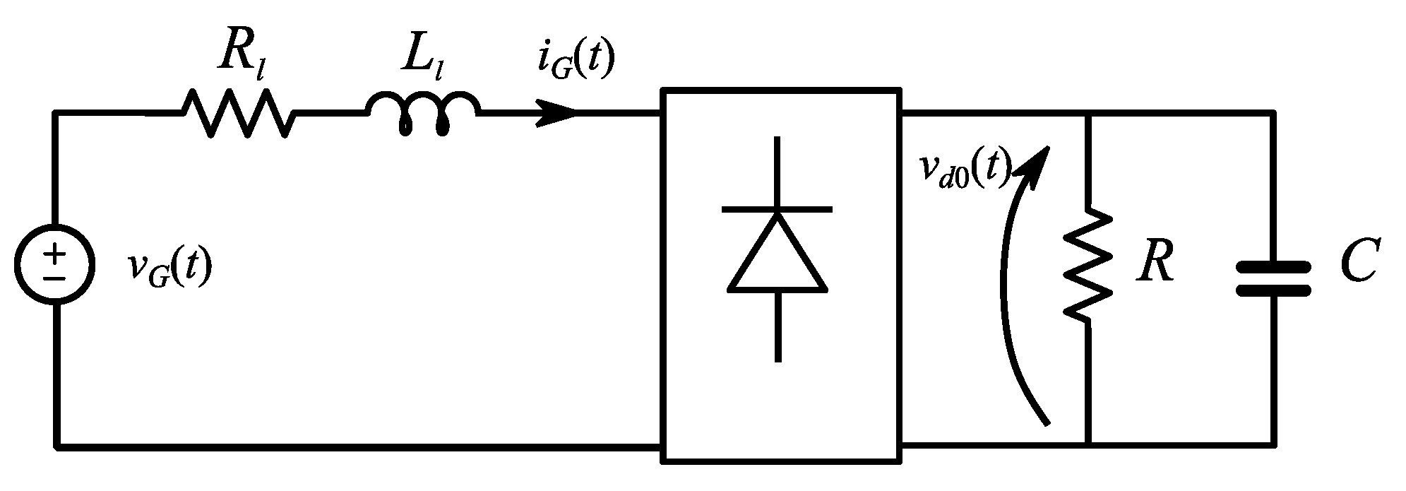
3. Case Study: Diode Bridge Rectifier

The target of this work is performing a comparison in terms of accuracy and complexity among X-parameters, FTM and simplified Volterra modeling approaches in representing the frequency-domain behavior of a strongly nonlinear device. The comparison will be carried out through numerical simulations, in order to avoid the impact of measurement uncertainty, which may mask the differences between different models. The selected case study consists of a diode rectifier feeding an ohmic-capacitive load, as shown in Figure 1: this architecture may represent the input stage of many devices connected to the distribution grid, such as battery chargers (including those for electric vehicles), PCs, household appliances and many others. The target is predicting current harmonics for a given input voltage spectrum. The resulting models, in conjunction with a proper frequency-domain solver, can be employed in order to study the propagation of harmonics in distribution grids.

Equivalent circuit parameters are listed in

Table 1. Parameters of the equivalent circuit.

VG,n (V)	Rl (Ω)	Ll (mH)	R (Ω)	C (mF)
53	0.4	4	50	1.41

(V_G,n represents the rated fundamental rms voltage) and diodes are represented with 0.8 V forward voltage drop and 1 mΩ resistance (no reverse conduction has been considered). The equivalent circuit has been implemented in MatLab/Simulink by using Simscape Power Systems library blocks. As aforementioned, the input u(t) is represented by the ac supply voltage v_G(t), while the resulting current i_G(t) corresponds to the model output y(t). Time-domain waveforms have been sampled with a sampling frequency f_s = 200 kS/s, which is a multiple of 50 Hz, in order to avoid the effect of leakage when spectra have to be computed through DFT, and high enough so that aliasing artifacts are negligible.

4. Model Identification

The three considered models have been identified according to the procedures explained in Section 2.

4.1. Frequency Transfer Matrix

Firstly, for estimating the FTM parameters, the reference condition has to be set: a pure sinewave voltage having a rated rms amplitude of V_G = 53 V and 50 Hz frequency. From the resulting steady-state current, the vector Y_B has been obtained. In order to estimate the tensor matrix, a set of voltage perturbations around the reference spectrum have been applied: R = 30 phase angles have been considered, while the amplitude of the perturbation has been set to ΔV_G(n) = 0.025 V_G for all the N input harmonics. This allows computing of the FTM model, whose parameters are obtained from Equation (9) and the procedure is reported in [12] and [16].

4.2. X-Parameters

Spectral linearization approximation has been applied by considering Q different LSOPs: Q has been varied from 1 to 5, in order to evaluate the accuracy improvement that can be reached by progressively increasing complexity. The Q LSOPs have been selected by dividing a supposed range of variation for the fundamental voltage (from 80% to 120% of the rated voltage in this case) into equal intervals. Once having defined all the LSOPs, the identification process explained in Section 2.2 has been carried out. Firstly, the response to the large signal components has been evaluated. Then 2(N−1) small-signal excitations have been generated, that is, two quadrature perturbations for each harmonic component; harmonic amplitude has been set to 2.5% of the fundamental. Then, Equation (15) has been applied to obtain X_S and X_T. Finally, in order to employ the identified model between different LSOPs, complex splines have been adopted to interpolate all the X-parameters values.

4.3. Simplified Volterra Model

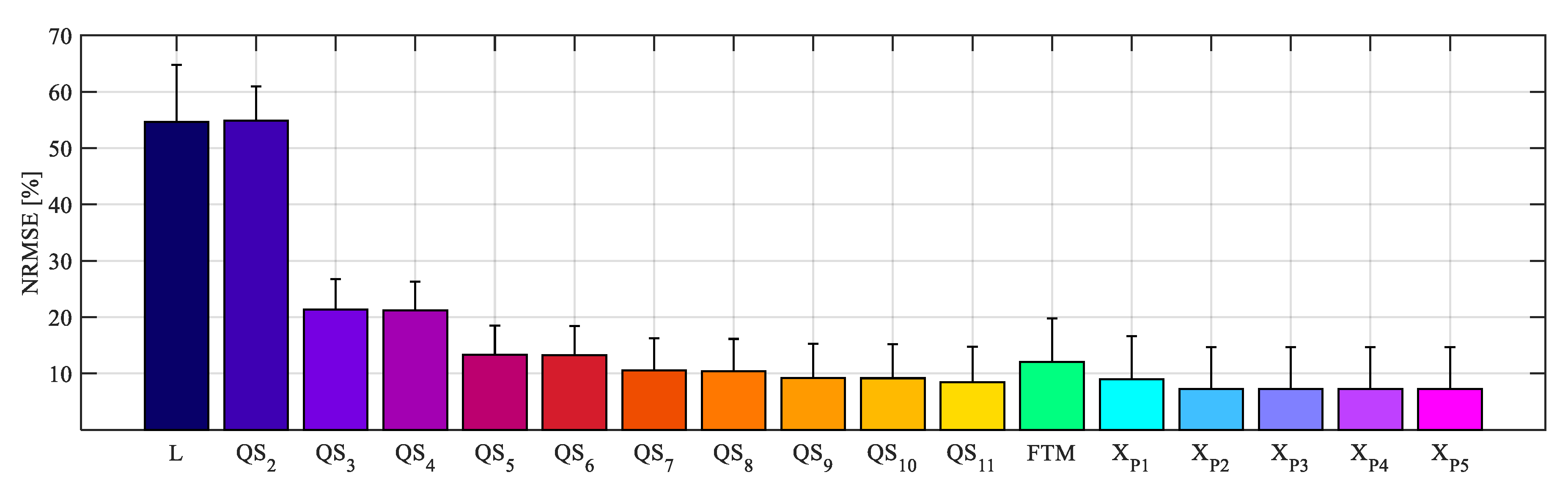
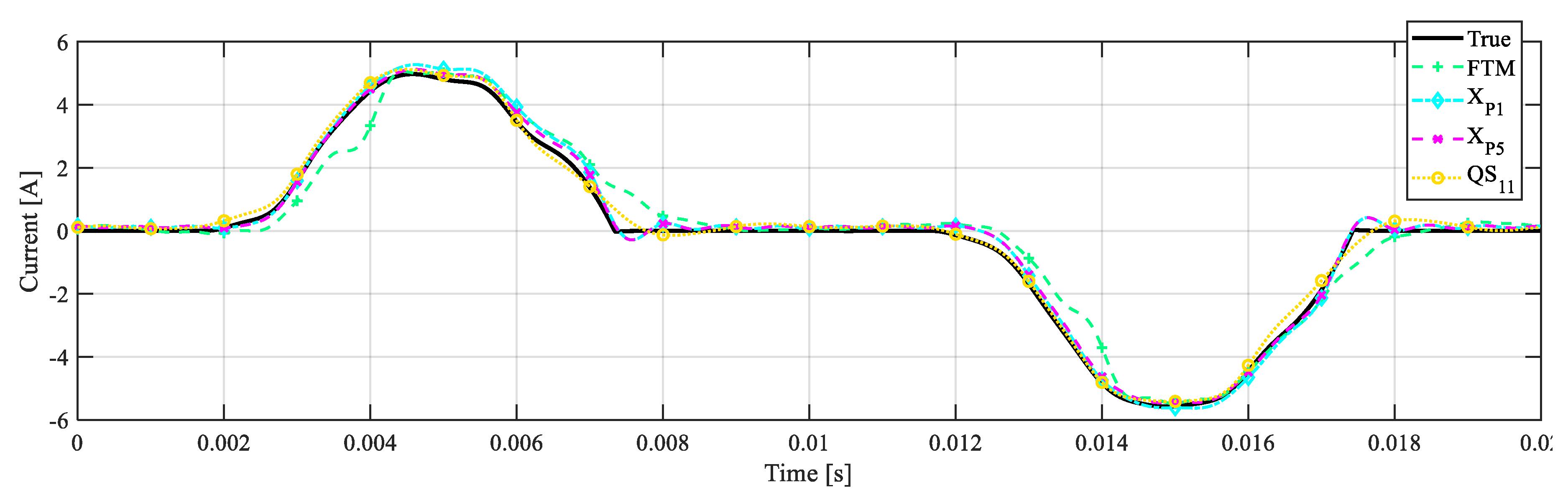
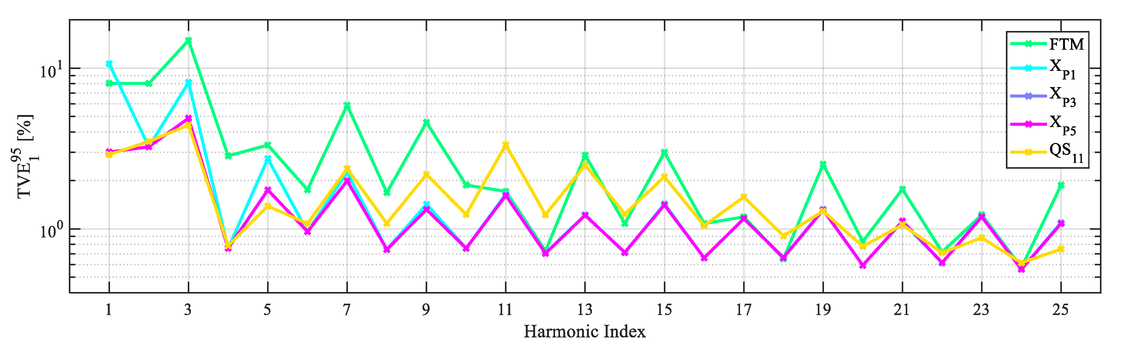
Simplified Volterra models characterized by I = 1 (linear model) to I = 11 have been estimated. In order to perform the identification, a set of P = 2000 test voltages resulting in full column rank matrix W_id(m) has been injected. Each pth voltage is characterized by a random fundamental amplitude (varying between 80% and 120% of the rated grid voltage), and N harmonics with both random amplitude (from 2% to 3% of the fundamental) and phases (between −π and π). Uniform independent pdfs have been considered.

The corresponding set of P steady-state currents waveforms i_G(t) has been obtained. The coefficient vectors H(m) have been estimated according to Equation (21).

5. Model Comparison

5.1. Random Fundamental Amplitude

A comparison of between the accuracy achieved by the different nonlinear approaches has been performed. This has been carried out by applying a proper set of realistic voltages (albeit different with respect to those adopted to estimate the model parameters), while comparing the currents predicted by the different behavioral models with those obtained by the reference circuit model.

A possible class of validation signals can be defined starting from the limits for harmonic voltages in public electricity networks prescribed by [31]. In particular, the 10 min rms value of each voltage harmonic has to be lower than the corresponding limit for 95% of the time over a one-week observation interval. Therefore, these limits can be reasonably considered as the 95th percentile bounds for harmonic amplitudes. However, no information about the shape of the probability density functions is provided in the standard; additional assumptions have to be introduced. Harmonic components are assumed to follow circular symmetric complex normal distributions, that amplitudes follow Rayleigh distributions (parameters are obtained from the respective limits), while phases are uniformly distributed in the range [−π; π]. A normally distributed fundamental amplitude has been supposed; its expectation is assumed to be equal to the rated voltage V_G,n. Ref. [31] states that the 10 min root mean square value of the voltage amplitude should be within 90% and 110% of the rated value for 95% of the time, considering a one-week observation time. Hence, these values have been employed as the 2.5th and 97.5th percentile values for the fundamental amplitude, so that the standard deviation of its distribution can be easily obtained. In order to perform the comparison, a set of P = 2000 random signals sampled from the previous defined pdfs has been applied to the behavioral models, and to the circuit model of the bridge rectifier.

An overall performance indicator is represented by the Normalized Root Mean Square Error (NMRSE). For the generic pth validation signal and model *, the NMRSE^[p] is defined as

$${\mathrm{NRMSE}}_{*}^{\left[p\right]}=\sqrt{\frac{{\displaystyle \sum _{k=1}^M{\left(i_{G,*}^{\left[p\right]}\left(k{T}_S\right)-i_G^{\left[p\right]}\left(k{T}_S\right)\right)}^2}}{{\displaystyle \sum _{k=1}^M{\left(i_G^{\left[p\right]}\left(k{T}_S\right)\right)}^2}}}$$

(22)

where i_G^[p] is the current evaluated by the circuit model when the pth validation signal is applied, while i_G,*^[p] is the corresponding prediction obtained with the validation signal. T_s is the sampling interval, and M = f_s/f₀ is the number of samples per period. An equivalent frequency-domain expression can be also derived. In Figure 2 the mean values and the 95th percentile bounds over the P test signals have been reported for each considered nonlinear model.

Considering a linear model (L in Figure 2), the achieved accuracy is clearly not acceptable: the average NRMSE reaches 55%, while the 95th percentile value is equal to 65%. On the contrary, the simplified Volterra models (QS_I, I = 1 … 11 in Figure 2) allows dramatically reducing these errors as long the degree is increased; as an example, the 11th degree model achieves a mean and a 95th percentile NRMSE of 9% and 15%, respectively. However, it is worth highlighting that passing from an odd-order degree model to the next even-order one has no impact on the NRMSE. The reason is clear since, because of its structure, the bridge rectifier can introduce purely odd-order nonlinearity.

When analyzing the performance of the FTM approach, it can be seen that its accuracy is worse with respect to the 11th degree Volterra model: in this case, the NRMSE is characterized by a mean value of 12% and a 95th percentile value of 20%. Finally, let us consider the X-parameters models with LSOPs varying from 1 to 5: when Q = 1, the model achieves a mean value and a 95th percentile of NRMSE, which are 9% and 16.6%, respectively, thus, slightly lower than FTM approach. Two LSOPs X-parameter model results in a minor accuracy improvement, with a mean NRMSE of 7.27% and a 95th percentile NRMSE of 14.6%. Increasing the number of LSOPs up to five does not significantly reduce these values.

In order to find the best trade-off between accuracy and complexity among all the presented nonlinear models, the total number of complex coefficients defining the considered models is shown in Figure 3.

Let us consider the simplified Volterra model: the number of coefficients grows with the square of nonlinearity degree, thus reaching 1470 when I = 11. The number of coefficients defining the X-parameters model is proportional to the number of the LSOPs, and each model is characterized by 1177 coefficients for each LSOP. Finally, the FTM model requires 1275 coefficients.

Now, let us focus on the 11th degree simplified Volterra model (defined by c_QS = 1470 coefficients), on the FTM approach (c_FTM = 1275) and on X-Parameters models with Q = 1, 3, 5 (c_X = 1177Q). First of all, the corresponding time-domain reconstructions of the current waveform have been obtained and compared with that of the reference circuit model. A random signal among the P tests have been randomly selected, and the result is depicted in Figure 4. It can be clearly noticed that the reconstruction provided by the FTM model shows a high deviation from the true value, especially outside the peaks. In fact, it is also the considered behavioral model resulting in the highest NRMSE values. The X-parameter model with Q = 1 provides a significantly better current waveform reconstruction, but errors near the peak are noticeable. On the other hand, the simplified Volterra model and the X-parameters approach with Q > 2 are more accurate over the entire period.

After that, the accuracy of the models in predicting current harmonics has been quantified. To this purpose, the Total Vector Error (TVE) has been computed for each mth order output harmonic and pth test signal. It corresponds to the distance in the complex plane between each current harmonic phasor obtained with the reference circuit model, and the corresponding prediction obtained by using the different behavioral models. It has been expressed in relative value with respect to the amplitude of the fundamental component:

$${\mathrm{TVE}}_1^{\left[p\right]}\left(m\right)=\frac{\left|I_{G,*}^{\left[p\right]}\left(m\right)-I_G^{\left[p\right]}\left(m\right)\right|}{\left|I_G^{\left[p\right]}\left(1\right)\right|}$$

(23)

In Figure 5, the 95th percentiles of the TVE₁ values evaluated over the P test signals for the different models (TVE₁⁹⁵) have been reported.

Figure 4 shows that the FTM model (green line) is generally the least accurate behavioral representation, especially for low order harmonics: the 95th percentile value of TVE₁ is always higher than 1.5% in this case. However, at the fundamental component the X-parameters approach with a single LSOP achieves the highest error, with TVE₁⁹⁵ exceeding 10%: this result is somewhat expected, since it is not capable to consider the variation of the fundamental component. Conversely, for the other harmonics it reaches a good accuracy, significantly better than that obtained with the FTM approach: TVE₁⁹⁵ is lower than 2% for harmonic orders greater than three. When increasing the number of LSOPs to three, the X-parameter model significantly improves the accuracy in predicting low-order current components. As far as the fundamental, TVE₁⁹⁵ drops from above 10% to about 3%. As already noticed when the NRMSEs have been compared, further increasing the number of LSOPs does not increase accuracy. The simplified Volterra model is able to perform similarly as the X-parameters approach with Q = 3 at low-order and high-order harmonics (albeit with a considerably smaller number of coefficients), but not in the middle part of the spectrum.

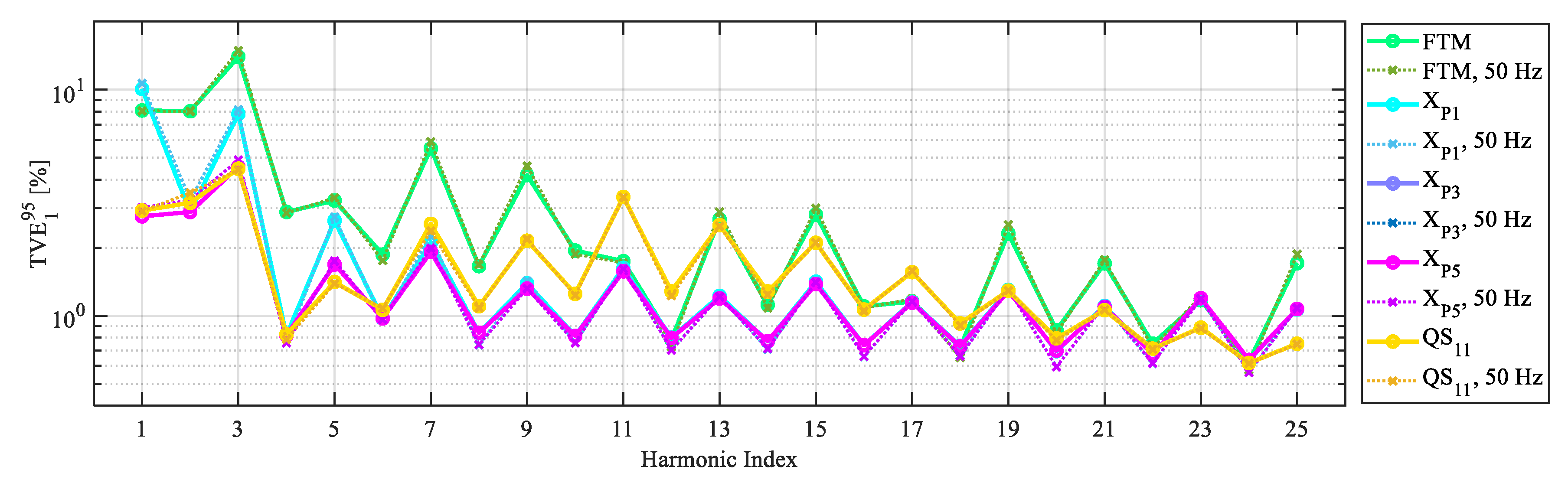
5.2. Random Fundamental Amplitude and Frequency

The previous validation has been performed considering rated fundamental frequency. Actually, grid voltages and currents are characterized by a fundamental frequency that may slightly deviate from nominal conditions. For this reason, it is interesting to evaluate the performances of the different methods when a class of signals having random but realistic fundamental frequency is considered. Standard EN 50160 [31] not only provides limits on harmonic amplitudes, but also states that the fundamental frequency must be within the range 49.5–50.5 Hz.

Therefore, P = 2000 signals have been randomly extracted with the same amplitude and phase distribution as in the previous case, but in this case also the fundamental frequency has been considered as a random variable having uniform distribution in the range prescribed by [31]. The sampling rate has been adjusted in order to have M = 4000 samples per fundamental period, thus guaranteeing synchronous sampling. As for the previous class of validation signals, the TVE₁ has been computed for each pth test signal and mth harmonic component. Its 95th percentile value has been computed (continuous lines) and compared with that obtained with the previous class of validation signals having fixed fundamental frequency (dotted lines). Results are reported in Figure 6.

From Figure 6, it can be concluded that all the models are robust with respect to small but realistic variations of the fundamental frequency. TVE₁⁹⁵ values obtained considering FTM, Volterra and X-parameter model with Q = 1 are completely overlapped to the results achieved with fixed fundamental frequency. A rather small variation is present when X-parameters models with Q = 3 and Q = 5 are considered. In this case, the highest variation occurs at the 20th order harmonic component, whose TVE₁⁹⁵ value increases from 0.5% to 0.6%, but it remains still lower with respect to that reached by the other models. For all the other harmonics, the differences in terms of TVE₁⁹⁵ are below 0.1%.

6. Conclusions

Harmonic simulations are extremely important in order to study and predict the impact of nonlinear devices on power quality. However, they require computationally effective models able to represent the nonlinear behavior of power system devices with adequate accuracy level. The target of this paper is comparing different behavioral, frequency-domain approaches that can be adopted for the purpose: X-parameters, FTM models and simplified Volterra models under quasi-sinusoidal conditions. A bridge rectifier feeding an ohmic-capacitive dc load have selected as case study, since it may represent the input stage of a wide class of devices connected to the distribution grid. The current voltage relationship defined by its circuit model has been represented by the considered behavioral approaches. After identification, their performances have been quantified by applying a class of realistic random voltages, while evaluating the quality of the current reconstructions. Results clearly show that the FTM approach is significantly affected by the variation of the fundamental component, while the X-parameters approach allows exemplary performance when different LSOPs are considered, but the number of coefficients increases noticeably. The 11th degree simplified Volterra model guarantees an accuracy which is close to that can be achieved by with the X-Parameters approach, but complexity is considerably lower. In fact, the 11th degree simplified Volterra model is defined by less than half of the coefficients required by X-Parameters models. Finally, accuracy under off-nominal frequency conditions have been evaluated; the achieved results highlights that the investigated models can be employed also in this case with marginal performance degradation.

References

1. Misra, R.; Paudyal, S.; Ceylan, O.; Mandal, P. Harmonic Distortion Minimization in Power Grids with Wind and Electric Vehicles. Energies 2017, 10, 932. [Google Scholar] [CrossRef] [Green Version]
2. Mastny, P.; Moravek, J.; Vojtek, M.; Drapela, J. Hybrid Photovoltaic Systems with Accumulation—Support for Electric Vehicle Charging. Energies 2017, 10, 834. [Google Scholar] [CrossRef] [Green Version]
3. Arrillaga, J.; Smith, B.C.; Watson, N.R.; Wood, A.R. Power System Harmonic Analysis; Wiley: New York, NY, USA, 1997. [Google Scholar]
4. Acha, E.; Madrigal, M. Power System Harmonics: Computer Modelling and Analysis; Wiley: Hoboken, NJ, USA, 2001. [Google Scholar]
5. IEEE Task Force on Harmonic Modeling and Simulation. Modeling and simulation of the propagation of harmonics in electric power systems Part I: Concepts, models, and simulation techniques. IEEE Trans. Power Deliv. 1996, 11, 452–464. [Google Scholar] [CrossRef]
6. IEEE Task Force on Harmonic Modeling and Simulation. Modeling and simulation of the propagation of harmonics in electric power systems Part II: Sample systems and examples. IEEE Trans. Power Deliv. 1996, 11, 466–474. [Google Scholar] [CrossRef]
7. IEEE Task Force on Harmonic Modeling and Simulation. Harmonic analysis in frequency and time domain. IEEE Trans. Power Deliv. 2013, 28, 1813–1821. [Google Scholar] [CrossRef]
8. Kundert, K.S.; Sangiovanni-Vincentelli, A. Simulation of nonlinear circuits in the frequency domain. IEEE Trans. Comput.-Aided Des. Integr. Circuits Syst. 1986, 5, 521–535. [Google Scholar] [CrossRef]
9. Kundert, K.S.; Sorkin, G.B.; Sangiovanni-Vincentelli, A. Applying harmonic balance to almost-periodic circuits. IEEE Trans. Microw. Theory Tech. 1988, 36, 366–378. [Google Scholar] [CrossRef]
10. Gilmore, R.J.; Steer, M.B. Nonlinear circuit analysis using the method of harmonic balance—A review of the art. Part I. Introductory concepts. Int. J. Microw. Millim.-Wave Comput.-Aided Eng. 1991, 1, 22–37. [Google Scholar] [CrossRef]
11. Fauri, M. Harmonic modelling of non-linear load by means of crossed frequency admittance matrix. IEEE Trans. Power Syst. 1997, 12, 1632–1638. [Google Scholar] [CrossRef]
12. Smith, B.C.; Watson, N.R.; Wood, A.R.; Arrillaga, J. Harmonic tensor linearisation of HVDC converters. IEEE Trans. Power Deliv. 1998, 13, 1244–1250. [Google Scholar] [CrossRef]
13. Yong, J.; Chen, L.; Chen, S. Modeling of Home Appliances for Power Distribution System Harmonic Analysis. IEEE Trans. Power Deliv. 2010, 25, 3147–3155. [Google Scholar] [CrossRef]
14. Zhou, N.; Wang, J.; Wang, Q.; Wei, N. Measurement-Based Harmonic Modeling of an Electric Vehicle Charging Station Using a Three-Phase Uncontrolled Rectifier. IEEE Trans. Smart Grid 2015, 6, 1332–1340. [Google Scholar] [CrossRef]
15. Yong, J.; Chen, L.; Nassif, A.B.; Xu, W. A Frequency-Domain Harmonic Model for Compact Fluorescent Lamps. IEEE Trans. Power Deliv. 2010, 25, 1182–1189. [Google Scholar] [CrossRef]
16. Caicedo, J.E.; Romero, A.A.; Zini, H.C. Frequency domain modeling of nonlinear loads, considering harmonic interaction. In Proceedings of the 2017 IEEE Workshop on Power Electronics and Power Quality Applications (PEPQA), Bogota, Colombia, 31 May–2 June 2017; pp. 1–6. [Google Scholar]
17. Root, D.E.; Verspecht, J.; Horn, J.; Marcu, M. X-Parameters: Characterization, Modeling, and Design of Nonlinear RF and Microwave Components; Cambridge University Press: Cambridge, UK, 2013. [Google Scholar]
18. Baylis, C.; Marks, R.J.; Martin, J.; Miller, H.; Moldovan, M. Going Nonlinear. IEEE Microw. 2011, 12, 55–64. [Google Scholar] [CrossRef]
19. Verspecht, J.; Williams, D.F.; Schreurs, D.; Remley, K.A.; McKinley, M.D. Linearization of large-signal scattering functions. IEEE Trans. Microw. Theory Tech. 2005, 53, 1369–1376. [Google Scholar] [CrossRef]
20. Verspecht, J.; Root, D.E. Polyharmonic distortion modeling. IEEE Microw. 2006, 7, 44–57. [Google Scholar] [CrossRef]
21. Verspecht, J. Describing Functions Can Better Model Hard Nonlinearities in the Frequency Domain Than the Volterra Theory. Ph.D. Thesis, Vrije Universiteit Brussel, Brussels, Belgium, November 1995. [Google Scholar]
22. Uhl, R.; Mirz, M.; Vandeplas, T.; Barford, L.; Monti, A. Non-linear behavioral X-Parameters model of single-phase rectifier in the frequency domain. In Proceedings of the IECON 2016—42nd Annual Conference of the IEEE Industrial Electronics Society, Florence, Italy, 23–26 October 2016; pp. 6292–6297. [Google Scholar]
23. Mirz, M.; Uhl, R.; Vandeplas, T.; Barford, L.; Monti, A. Measurement-based parameter identification of non-linear polynomial frequency domain model of single-phase four diode bridge rectifier. In Proceedings of the 2017 IEEE International Instrumentation and Measurement Technology Conference (I2MTC), Turin, Italy, 22–25 May 2017; pp. 1–6. [Google Scholar]
24. Faifer, M.; Ottoboni, R.; Prioli, M.; Toscani, S. Simplified Modeling and Identification of Nonlinear Systems Under Quasi-Sinusoidal Conditions. IEEE Trans. Instrum. Meas. 2016, 65, 1508–1515. [Google Scholar] [CrossRef]
25. Faifer, M.; Laurano, C.; Ottoboni, R.; Prioli, M.; Toscani, S.; Zanoni, M. Definition of Simplified Frequency-Domain Volterra Models with Quasi-Sinusoidal Input. IEEE Trans. Circuits Syst. I 2018, 65, 1652–1663. [Google Scholar] [CrossRef]
26. Faifer, M.; Laurano, C.; Ottoboni, R.; Toscani, S.; Zanoni, M. Behavioral Representation of a Bridge Rectifier Using Simplified Volterra Models. IEEE Trans. Instrum. Meas. 2019, 68, 1611–1618. [Google Scholar] [CrossRef]
27. Faifer, M.; Laurano, C.; Ottoboni, R.; Toscani, S.; Zanoni, M. Modeling and identification of a bridge rectifier under quasi-sinusoidal conditions. In Proceedings of the 2018 IEEE International Instrumentation and Measurement Technology Conference (I2MTC), Houston, TX, USA, 14–17 May 2018; pp. 1–5. [Google Scholar]
28. Faifer, M.; Laurano, C.; Ottoboni, R.; Toscani, S.; Zanoni, M.; Crotti, G.; Giordano, D.; Barbieri, L.; Gondola, M.; Mazza, P. Overcoming Frequency Response Measurements of Voltage Transformers: An Approach Based on Quasi-Sinusoidal Volterra Models. IEEE Trans. Instrum. Meas. 2018, 68, 2800–2807. [Google Scholar] [CrossRef]
29. Collin, A.J.; Djokic, S.Z.; Drapela, J.; Langella, R.; Testa, A. Light Flicker and Power Factor Labels for Comparing LED Lamp Performance. IEEE Trans. Ind. Appl. 2019, 55, 7062–7070. [Google Scholar] [CrossRef] [Green Version]
30. Femia, N.; di Capua, G.; Ohashi, R.A.P. Harmonic analysis of diode-bridge rectifiers in Wireless Power Transfer System. In Proceedings of the 2017 14th International Conference on Synthesis, Modeling, Analysis and Simulation Methods and Applications to Circuit Design (SMACD), Giardini Naxos, Italy, 12–15 June 2017; pp. 1–4. [Google Scholar]
31. Voltage Characteristics of Electricity Supplied by Public Electricity Networks, Standard EN 50160; CENELEC: Brussels, Belgium, 2010.
Figure 1. Circuit model of the considered case study.
Energies 13 02609 g001
Figure 2. Normalized Root Mean Square Error (NRMSE) mean value and 95th percentile values for each considered model.
Energies 13 02609 g002
Figure 3. NRMSE mean value and 95th percentile values for each considered model.
Energies 13 02609 g003
Figure 4. Time-domain reconstruction of iG for the different models.
Energies 13 02609 g004
Figure 5. Total Vector Error (TVE)1 95th percentile values for the different behavioral models.
Energies 13 02609 g005
Figure 6. TVE1 95th percentile bands for the different behavioral models, random fundamental frequency.
Energies 13 02609 g006