ForecastTB—An R Package as a Test-Bench for Time Series Forecasting—Application of Wind Speed and Solar Radiation Modeling

Abstract

This paper introduces an R package ForecastTB that can be used to compare the accuracy of different forecasting methods as related to the characteristics of a time series dataset. The ForecastTB is a plug-and-play structured module, and several forecasting methods can be included with simple instructions. The proposed test-bench is not limited to the default forecasting and error metric functions, and users are able to append, remove, or choose the desired methods as per requirements. Besides, several plotting functions and statistical performance metrics are provided to visualize the comparative performance and accuracy of different forecasting methods. Furthermore, this paper presents real application examples with natural time series datasets (i.e., wind speed and solar radiation) to exhibit the features of the ForecastTB package to evaluate forecasting comparison analysis as affected by the characteristics of a dataset. Modeling results indicated the applicability and robustness of the proposed R package ForecastTB for time series forecasting.

1. Introduction

Decision making is one of the most crucial tasks in many domains and often decisions are based on the most accurate forecast available in the respective domains. A large number of areas, such as energy [1,2], economics [3], infrastructure [4,5], health [6,7], agriculture [8,9], defense [10], education [11,12], technology [13,14], geo-science [15], climate [16] and structural engineering [17] among several others, are looking forward to benefits that can be achieved with time series forecasting. Time series are consecutive sequences of values ordered with respect to time. Statistically, it is represented by the theory of stochastic processes [18]. The notable feature of time series data is the time-based correlation between values such that the probability of occurrence of a value depends on future or past observations [19,20].

Standardizing the process of the forecasting methods comparison is associated with numerous challenges [21]. The apparent concern is the nature of the time series and selection of appropriate methods such as the complete variation from seasonality, trends, and random parameters, that should be handled with each method. For instance, one forecasting model may perform better for a seasonal time series but show poor accuracy as compared to other models for a trendy or a random one [22]. Besides, interpretations might be affected by the error metric selection, for example, Root mean square error (RMSE), as different metrics have different objectives [23].

The ForecastTB package can be helpful for professionals and researchers working in the field of data science and forecasting analysis. The salient features of the ForecastTB package are as follows:

• Reduction in efforts and time consumption: The ForecastTB package is designed to reduce the efforts and time consumption for the time series forecasting analysis. It avoids the repetitive steps in the analysis and leads to the promising comparative results report generation.
• Truthful comparison assurance: The ForecastTB package ensures a truthful and unbiased comparison of forecasting methods. Hence, this package may be considered a reliable tool for forecasting models based on industrial reports generation or scientific publications.
• Reproducible research: Along with unbiased comparisons, the ForecastTB package provides ease in reproducible research with minimum efforts. In other words, the forecasting comparison can be reproduced several times easily with the help of the ForecastTB package.
• Stepping stone in machine learning automation: Forecasting methods play a very important role in machine learning applications [24]. The ForecastTB package aims to evaluate the best performing forecasting method for a given time series dataset and this can be presented as a stepping stone in machine learning automation modeling. For example, on changing nature and patterns of the time series dataset, a machine learning application could automatically replace the existing forecasting methods based on the output of the ForecastTB package.
• A handy tool: The ForecastTB package is a handy tool, especially for researchers who are not comfortable with computer coding, since it is a plug-and-play module based package. A very simple syntax leads to very impressive and accurate forecasting comparison analysis.

This paper demonstrates the inspection of the ForecastTB package as a testbench for the comparative study of different forecasting methods [25]. The motivation behind this package is another R package, named imputeTestbench [26,27], which demonstrated great success in performing comparison analysis with time series imputation methods in several research studies [28,29,30,31]. The ForecastTB package aims at providing an evaluation toolset that overcomes the challenges of discovering the most suitable forecasting method along with a detailed comparative analysis. This package allows simulating random possibilities of different strategies including Monte-Carlo simulation. Values forecasted with several different methods are then compared with a user defined error metric. A couple of plotting functions are provided for overall forecast evaluation visualization. Besides, demonstration examples and case studies on natural time series datasets are discussed to showcase the usage of ForecastTB package.

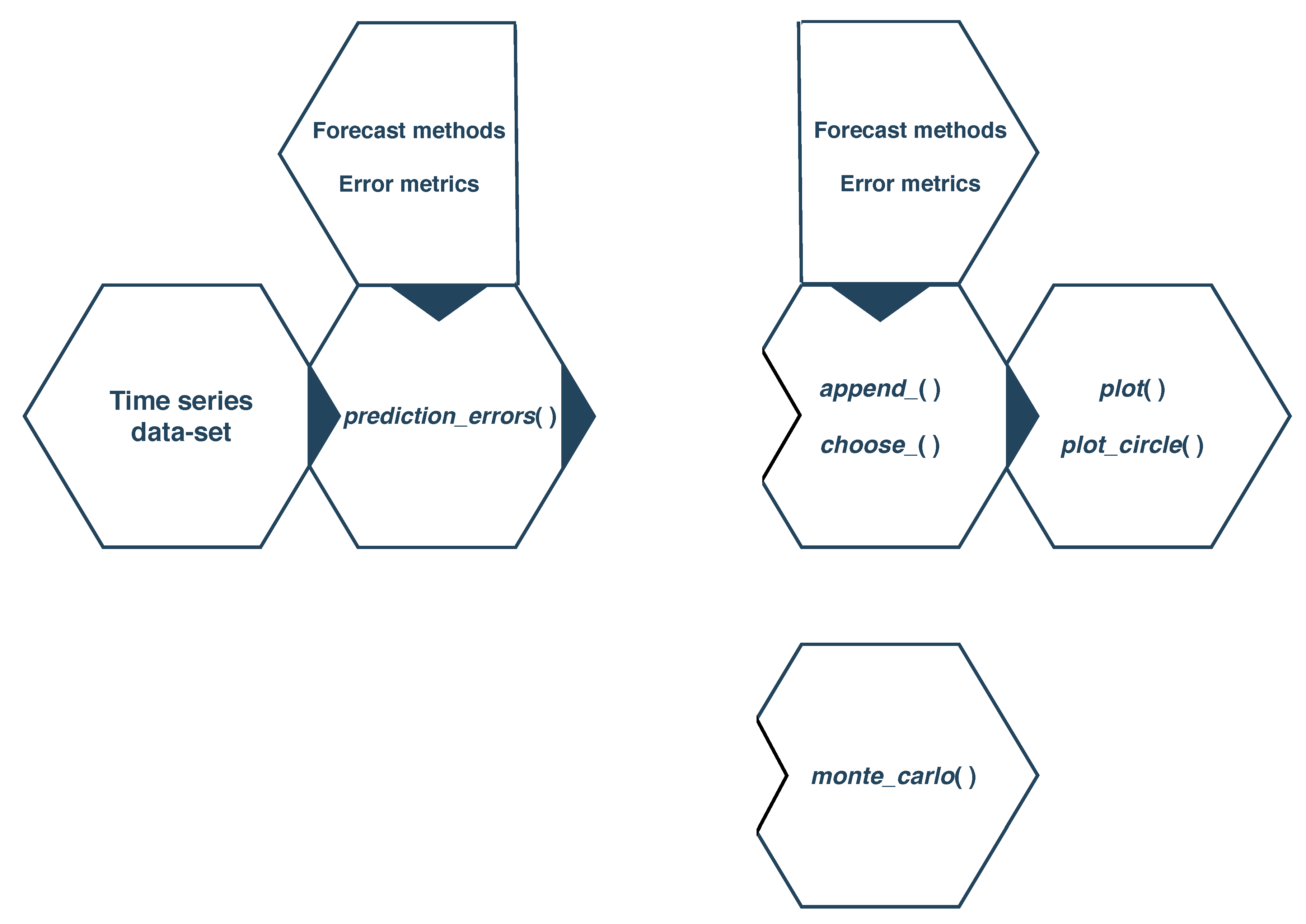
2. Overview of ForecastTB

The ForecastTB package is a plug-and-play structured module as shown in Figure 1. It is used to compare the forecasting methods, which begins by forecasting time series with distinct strategies. Then the prediction accuracies are evaluated with the error metrics for all methods for several repetitions. The prediction_errors() function is employed for a forecasting method comparative evaluation with the consideration of various input parameters. It returns an object, which is the basic module in the package. Further this module can be updated with new methods and other parameters with append_() and choose_() functions. The Monte_Carlo() function is a further extension of the prediction_errors() module to compare distinct methods for randomly selected patches of the input time series. The remaining two functions, plotMethods() and plot_circle(), are used to visualize forecasted results and error summaries for the chosen methods. All functions, as a set of modules, are based on and connected with the object provided by the prediction_errors() function. Hence, the framework of the ForecastTB package is version-control-friendly. It means, in the future, new features in the next versions of the package, can be easily introduced.

Dependencies include additional packages for data manipulation (reshape2, [32]; stats, [33]), graphing (ggplot2, [34]; circlize, [35]; graphics, [33]; gridExtra, [36]; RColorBrewer, [37]), and forecast (forecast, [38]; PSF, [39,40,41]; decomposedPSF, [42]; methods, [33]).

Recently, a package in R was proposed for streamlining time series forecasting with limited facilities and features, named as predtoolsTS [43,44]. This tool assists in forecasting with the automated Auto-Regressive Integrated Moving Average (ARIMA) model [38] and only regression type algorithms from the caret [45] package in the closed environment. Beyond this, there is no facility to append new forecasting methods and updating the comparison environment as per the user’s need. On the contrary, the proposed ForecastTB package provides such multiple facilities along with the possibilities of introducing new features with a simple plug-and-play structure as discussed in the article.

2.1. The prediction_errors() function

The prediction_errors() is a primary function that compares the performance of different forecasting methods depends on various parameters supplied by user. The default methods included in prediction_errors() are ARIMA from the forecast package [38] and the Pattern sequence based forecast (PSF) method from the PSF package [39,40]. This statistical method, ARIMA, is most widely and frequently used in time series forecasting. It is comfortably modeled as compared to more complex approaches. Moreover, to avoid further complexity, the auto.arima() function in the forecast package [38] and psf() from the PSF package are used, which automatically estimates the model parameters required for the given dataset. With the following examples, we show the possibility of adding extra and user-defined methods as needed.

Following are the arguments of the prediction_errors() function:

a <- prediction_errors(data = data, nval = 12,

          ePara = c(’RMSE’, ’MAE’), ePara_name = c(’RMSE’, ’MAE’),

          Method = c(’ARIMA’, ’PSF’), MethodName = c(’ARIMA’, ’PSF’),

          strats = ’Recursive’, dval = length(data),

          append_ = 0)

data:

A ts (stats) as input dataset (numeric object) to be evaluated. It is a time varied dataset for comparison of performance and accuracy of forecasting methods.

nval:

An integer value to decide a number of values to be predicted while comparing the forecasting methods. The default value is 12.

ePara:

The forecasted and observed values are compared with error metrics. The root-mean-squared error (RMSE), mean absolute error (MAE), and mean absolute percent error (MAPE) [46] are the default error metrics included in ForecastTB, but the individual metric can be opted using ePara = ‘rmse’, ‘mae’, or ‘mape’. The error metrics are defined as:

$$\mathrm{RMSE}=\sqrt{\frac{1}{\mathrm{N}}\sum _{\mathrm{i}=1}^{\mathrm{N}}{\left|{\mathrm{X}}_{\mathrm{i}}-{\widehat{\mathrm{X}}}_{\mathrm{i}}\right|}^2}$$

(1)

$$\mathrm{MAE}=\frac{1}{\mathrm{N}}\sum _{\mathrm{i}=1}^{\mathrm{N}}\left|{\mathrm{X}}_{\mathrm{i}}-{\widehat{\mathrm{X}}}_{\mathrm{i}}\right|$$

(2)

$$\mathrm{MAPE}=\frac{1}{\mathrm{N}}\sum _{\mathrm{i}=1}^{\mathrm{N}}\frac{\left|{\mathrm{X}}_{\mathrm{i}}-{\widehat{\mathrm{X}}}_{\mathrm{i}}\right|}{{\mathrm{X}}_{\mathrm{i}}}\times 100\%,$$

(3)

where ${\mathrm{X}}_{\mathrm{i}}$ and ${\widehat{\mathrm{X}}}_{\mathrm{i}}$ are the observed and forecasted data at time $\mathrm{t}$, respectively. $\mathrm{N}$ is the number of data for forecast evaluation.

Additionally, a new error metric of the user’s choice can be introduced in the following manner: ePara = c("errorparametername"), where errorparametername is an external function which returns desired error values for original and forecasted values. It is discussed in detail in the following sections.

ePara_name:

A string of characters for the names of error metrics provided in ePara. In the prediction_errors() function, RMSE, MAE and MAPE are the default names for the error parameters.

Method:

A string with method names that are used to forecast values with ARIMA, PSF and user-defined methods. The ARIMA is a default method until the user changes it. For instance, Method = c("PSF") will use only the PSF with the prediction_errors() function. New forecasting methods can be included in prediction_errors() function with Method = c("test1(data, nval)") vector, where test1 is an external function which forecasts nval number of future values for input data and returns the forecasted values. Such multiple functions can be added in the Method parameter. The external function is expected to provide forecast methods using the recursive strategy.

MethodName:

A string of characters provided by user as one or more forecast methods passed to Method. The default list of name of method in the prediction_errors() function is ARIMA.

strats:

A character string of names of forecasting strategies used for time series forecasting. The strategies used in the current version of the prediction_errors() function are Recursive and DirRec. In the recursive approach, the first value is predicted with a prediction model and then appended to the data-set. Fits to the same model are then used to predict the next value. In the DirRec approach, the first value is predicted with a model and appended it to the data-set. A new model is then fitted and used to predict the next value and so on. The default strategy in the prediction_errors() function is the Recursive one.

append_:

A flag that suggests if the function is used to append to another instance. The default flag is 1, which indicates newly added methods are compared with the default methods. When the flag is 0, all methods, excluding default methods, will be compared.

dval:

An integer that specifies the length of the data subset to be used for forecasting. The default value is the length of the data parameter.

With the default entities for all arguments, the prediction_errors() function generates an S4 object of class prediction_errors as the error profile for the forecasting methods. This prediction_errors() function returns two slots as output. The first slot is output, which provides Error_Parameters, indicating error values for the forecasting methods and error parameters defined in the framework, and Predicted_Values as values forecasted with the same foreasting methods. Further, the second slot is parameters, which returns the parameters used or provided to prediction_errors() function. This is illustrated in the following example:

## An object of class "prediction_errors"

## Slot "output":

## $Error_Parameters

##       RMSE    MAE    MAPE exec_time

## ARIMA 53.357458 45.662500  9.647511  1.248623

##

## $Predicted_Values

##           1     2     3    4     5    6     7

## Test values 417.0000 391.0000 419.0000 461.0000 472.0000 535.0000 622.0000

## ARIMA    425.5702 432.2525 489.0878 499.4493 539.9511 539.7919 536.0011

##           8    9    10    11    12

## Test values 606.000 508.0000 461.000 390.0000 432.0000

## ARIMA    525.408 492.9301 486.233 461.6871 470.2665

##

##

## Slot "parameters":

## $data

##    Jan Feb Mar Apr May Jun Jul Aug Sep Oct Nov Dec

## 1949 112 118 132 129 121 135 148 148 136 119 104 118

## 1950 115 126 141 135 125 149 170 170 158 133 114 140

## 1951 145 150 178 163 172 178 199 199 184 162 146 166

## 1952 171 180 193 181 183 218 230 242 209 191 172 194

## 1953 196 196 236 235 229 243 264 272 237 211 180 201

## 1954 204 188 235 227 234 264 302 293 259 229 203 229

## 1955 242 233 267 269 270 315 364 347 312 274 237 278

## 1956 284 277 317 313 318 374 413 405 355 306 271 306

## 1957 315 301 356 348 355 422 465 467 404 347 305 336

## 1958 340 318 362 348 363 435 491 505 404 359 310 337

## 1959 360 342 406 396 420 472 548 559 463 407 362 405

## 1960 417 391 419 461 472 535 622 606 508 461 390 432

##

## $nval

## [1] 12

##

## $ePara

## [1] "RMSE" "MAE"  "MAPE"

##

## $ePara_name

## [1] "RMSE" "MAE"  "MAPE"

##

## $Method

## [1] "ARIMA"

##

## $MethodName

## [1] "ARIMA"

##

## $Strategy

## [1] "Recursive"

##

## $dval

## [1] 144

2.2. The append_() and choose_() functions

The append_() and choose_() are functions to add new forecasting methods and choose the selected methods to and within the prediction_errors object. These functions make ForecastTB a handy plug-and-play tool for forecasting analysis. The append_() function has the following arguments:

append_(object = a,

    Method = c("test2(data,nval)"), MethodName = c(’Test2’),

    ePara = c(’RMSE’, ’MAE’), ePara_name = c(’RMSE’, ’MAE’))

object:

A prediction_errors object with two slots, output and parameters returned by the prediction_errors() function.

Method, MethodName, ePara and~ePara_name:

These parameters are with similar meaning as that supplied to the prediction_errors() function. The ePara and ePara_name parameters of the append_() function automatically get synced with the prediction_errors() function. The append_() function returns the error profile for the forecasting methods along with newly added ones in the form of an updated prediction_errors object.

Further, the choose_() function helps the user to manipulate the prediction_errors object, by allowing selection of the desired methods existing in the object. The choose_() function has the following argument:

choose_(object)

object:

A prediction_errors object returned by the prediction_errors() or append_() function. The syntax of the choose_() function is discussed in the following example. The variable c is an object with three forecasting methods comparisons. After provide the c object to the choose_() function, it returns the following output showing names of forecasting methods attached in the c object and asks the index number of method to be removed from the same object. Finally, it stores the newly updated object in the variable d.

## > d <- choose_(object = c)

## Following are the~methods attached with the~object:

##      [,1]  [,2]  [,3]

## Indices "1"   "2"  "3"

## Methods "ARIMA" "DPSF" "xyz"

## Enter the~indices of methods to remove:2

After removing on of the methods with the choose_() function, a new object d is returned as follows:

## > d@output

## $Error_Parameters

##       RMSE    MAE    MAPE exec_time

## ARIMA 2.3400915 1.9329816 4.2156087 0.1328349

## xyz  4.0909453 3.3250000 7.1517742 0.4336619

##

## $Predicted_Values

##           1     2     3    4     5    6     7    8

## Test values 39.40000 40.90000 42.40000 47.80000 52.40000 58.00000 60.70000 61.80000

## ARIMA    37.41933 37.69716 41.18252 46.29926 52.24804 57.10696 59.71674 59.41173

## xyz     44.20000 39.80000 45.10000 47.00000 54.10000 58.70000 66.30000 59.90000

##           9    10    11    12

## Test values 58.20000 46.7000 46.60000 37.80000

## ARIMA    56.38197 51.4756 46.04203 41.52592

## xyz     57.00000 54.2000 39.70000 42.80000

In this way, the append_() and choose_() functions provide features to manage the desired forecasting methods in the prediction_errors object with simple and single lined syntax. Besides, these functions avoid repetitive computation and execution of the methods which are already attached in the prediction_errors object.

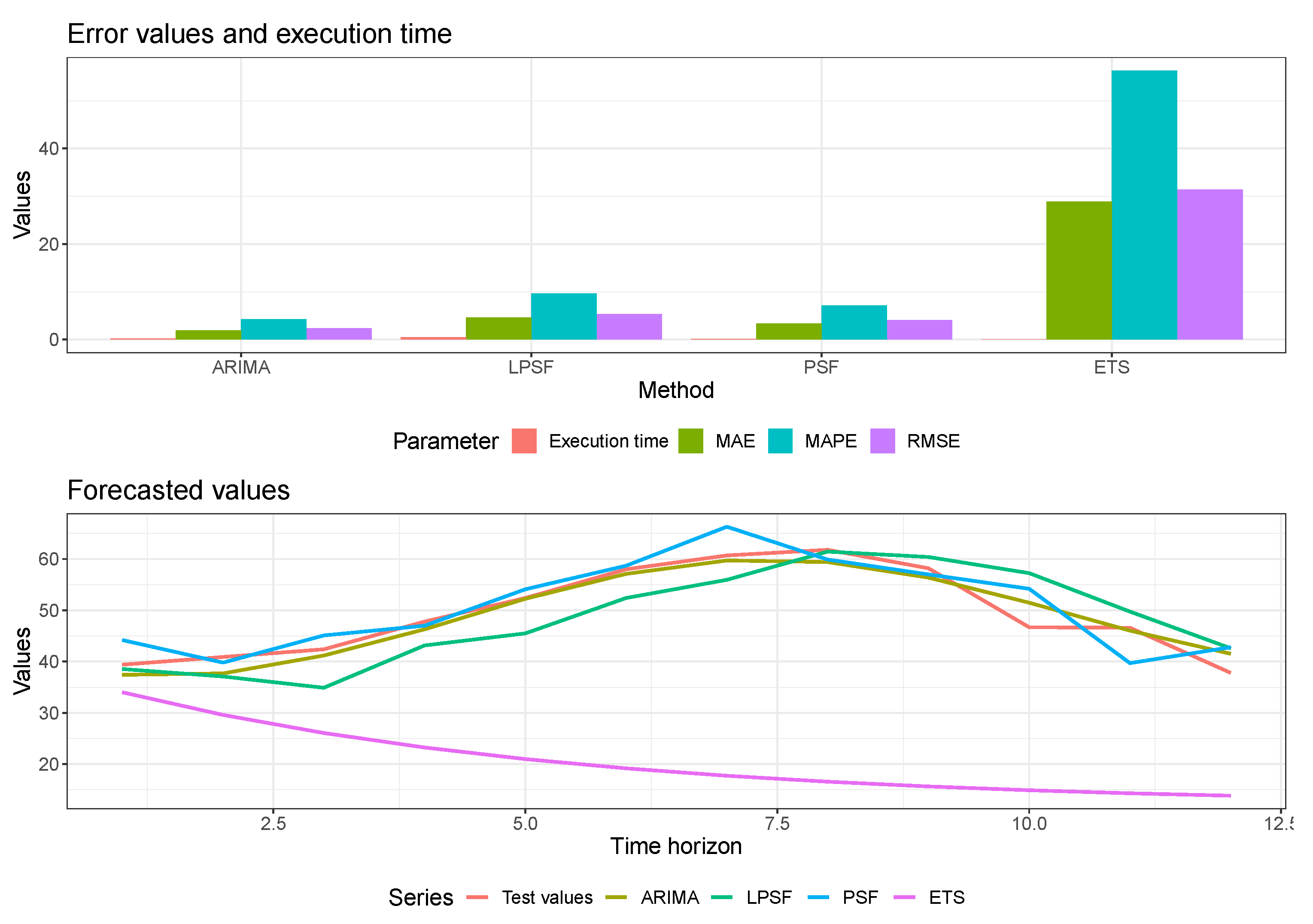
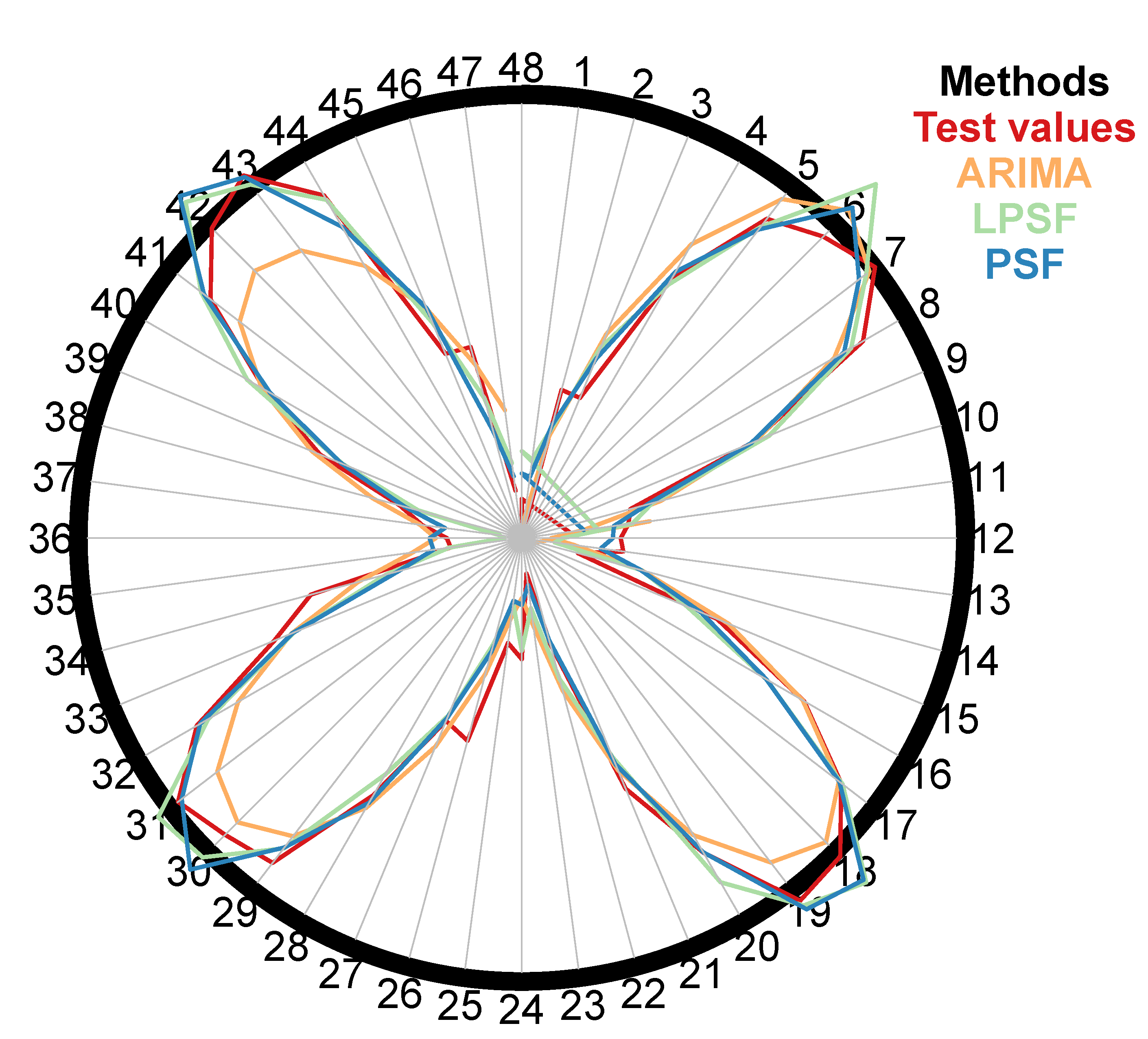
2.3. The plot.prediction_errors() and plot_circle() functions

The plot.prediction_errors() and plot_circle() functions allow users to plot the S4 object of the prediction_errors class. The plot.prediction_errors() is an S3 method, in which, along with the prediction_errors object, it optionally accepts other variables in used to describe plots in R, such as, legends, axes, labels, and so forth. This function plots a bar-chart of error values and execution time and line plots of forecasted values with significant color changes for different forecasted methods. The plot generated plot.prediction_errors() consists of a dynamic margin size with which forecasted values can be included if required. The plot.prediction_errors() function syntax and usage are discussed below:

plot.prediction_errors(object = a, ...)

Furthermore, the plot_circle() function provides a polar plot for showing forecasted values, especially if these are seasonal values. This plot shows how forecasted observations are behaving on an increasing number of seasonal time horizons. The syntax of the plot_circle() function is similar to that of plot.prediction_errors() one, as shown below:

plot_circle(object = a, ...)

2.4. The monte_carlo() function

Monte-Carlo sampling is a very popular strategy to compare the performance of forecasting methods. In this strategy, multiple patches of a dataset are selected randomly and then tests of the performance of the forecasting methods are executed. It returns the average of error values obtained for each data patches. The most notable feature of the Monte-Carlo strategy is that it ensures an accurate comparison of forecasting methods and avoids the biased results which might be obtained by chance.

The monte_carlo() function has the following arguments:

monte_carlo(object, size, iteration, fval, figs)

object:

An S4 object of the prediction_errors class with two slots, output and parameters returned by the prediction_errors(), append_() or choose_() functions. The monte_carlo() function tunes itself based on parameters returned by the object.

size:

An integer value representing the length of the patches from the time series dataset used in the Monte Carlo strategy. The input dataset is referred from the prediction_errors object.

iteration:

A numeric value representing the iterations to be used by the Monte-Carlo strategy.

fval:

A flag, when it is on (fval = 1), the monte_carlo() function return the output along with the forecasted values for each iteration. The default value of fval is 0, that returns only the error values in RMSE in each iteration.

figs:

A flag to plot with the plot.prediction_errors() function for each iteration in Monte-Carlo strategy when figs = 1. The default value of figs is 0 and it does not return any plots.

This way, the monte_carlo() function returns the error values along with the mean values for the provided forecasted methods in each iteration of the Monte-Carlo strategy. This function can be used as a quick tool to create an intuition of best-suited forecasting method for a given time series dataset.

3. A Case Study: Performance of Forecasting Methods on Standard Natural Time Series

This section presents a case study to introduce the use of the ForecastTB package as a test-bench to compare the performance of time series forecasting methods. The methods used in the case study are the auto.arima(), ets(), psf(), and lpsf() that are frequently used R functions for time series forecasting. The two standard datasets used in this example are nottem and sunspots. The nottem is the average air temperatures recorded at Nottingham Castle in degrees Fahrenheit from 1920 to 1930 (datasets package, [33]) Similarly, the sunspots is mean relative sunspot numbers from 1749 to 1983 (datasets package, [33]). Both datasets are measured on monthly basis.

In the following examples, the whole comparison analysis and visualization are done for the nottem dataset, but only the error values are shown for the sunspots dataset. The following are the two functions that represent forecasting methods. These methods include LPSF and PSF methods from the decomposedPSF [42] and PSF [39] packages. These functions consume time series dataset and nval as input parameters and return the forecasted values as a string.

The following code chunk is the main function in the ForecastTB package, in which performance of ARIMA along with the above mentioned (PSF and LPSF) methods are compared for the nottem time series for next 12 months forecast. The output of the function is saved in the variable a1 as an S4 object of prediction_errors class.

## An object of class "prediction_errors"

## Slot "output":

## $Error_Parameters

##       RMSE    MAE    MAPE exec_time

## ARIMA 2.3400915 1.9329816 4.2156087 0.2290468

## LPSF  5.3525306 4.5916667 9.6590830 0.2280521

## PSF   2.2454324 1.9450000 4.1462600 0.1007819

##

## $Predicted_Values

##           1     2     3    4     5    6     7

## Test values 39.40000 40.90000 42.40000 47.80000 52.40000 58.00000 60.70000

## ARIMA    37.41933 37.69716 41.18252 46.29926 52.24804 57.10696 59.71674

## LPSF     38.55000 37.10000 34.90000 43.15000 45.50000 52.40000 55.95000

## PSF     38.38000 37.56000 41.80000 45.46000 52.96000 57.14000 61.68000

##           8     9    10    11    12

## Test values 61.80000 58.20000 46.7000 46.60000 37.80000

## ARIMA    59.41173 56.38197 51.4756 46.04203 41.52592

## LPSF     61.45000 60.40000 57.2500 49.75000 42.60000

## PSF     59.20000 56.68000 49.6000 42.56000 40.38000

##

##

## Slot "parameters":

## $data

##     Jan Feb  Mar Apr  May Jun  Jul Aug  Sep Oct  Nov Dec

## 1920 40.6 40.8 44.4 46.7 54.1 58.5 57.7 56.4 54.3 50.5 42.9 39.8

## 1921 44.2 39.8 45.1 47.0 54.1 58.7 66.3 59.9 57.0 54.2 39.7 42.8

## 1922 37.5 38.7 39.5 42.1 55.7 57.8 56.8 54.3 54.3 47.1 41.8 41.7

## 1923 41.8 40.1 42.9 45.8 49.2 52.7 64.2 59.6 54.4 49.2 36.3 37.6

## 1924 39.3 37.5 38.3 45.5 53.2 57.7 60.8 58.2 56.4 49.8 44.4 43.6

## 1925 40.0 40.5 40.8 45.1 53.8 59.4 63.5 61.0 53.0 50.0 38.1 36.3

## 1926 39.2 43.4 43.4 48.9 50.6 56.8 62.5 62.0 57.5 46.7 41.6 39.8

## 1927 39.4 38.5 45.3 47.1 51.7 55.0 60.4 60.5 54.7 50.3 42.3 35.2

## 1928 40.8 41.1 42.8 47.3 50.9 56.4 62.2 60.5 55.4 50.2 43.0 37.3

## 1929 34.8 31.3 41.0 43.9 53.1 56.9 62.5 60.3 59.8 49.2 42.9 41.9

## 1930 41.6 37.1 41.2 46.9 51.2 60.4 60.1 61.6 57.0 50.9 43.0 38.8

## 1931 37.1 38.4 38.4 46.5 53.5 58.4 60.6 58.2 53.8 46.6 45.5 40.6

## 1932 42.4 38.4 40.3 44.6 50.9 57.0 62.1 63.5 56.3 47.3 43.6 41.8

## 1933 36.2 39.3 44.5 48.7 54.2 60.8 65.5 64.9 60.1 50.2 42.1 35.8

## 1934 39.4 38.2 40.4 46.9 53.4 59.6 66.5 60.4 59.2 51.2 42.8 45.8

## 1935 40.0 42.6 43.5 47.1 50.0 60.5 64.6 64.0 56.8 48.6 44.2 36.4

## 1936 37.3 35.0 44.0 43.9 52.7 58.6 60.0 61.1 58.1 49.6 41.6 41.3

## 1937 40.8 41.0 38.4 47.4 54.1 58.6 61.4 61.8 56.3 50.9 41.4 37.1

## 1938 42.1 41.2 47.3 46.6 52.4 59.0 59.6 60.4 57.0 50.7 47.8 39.2

## 1939 39.4 40.9 42.4 47.8 52.4 58.0 60.7 61.8 58.2 46.7 46.6 37.8

##

## $nval

## [1] 12

##

## $ePara

## [1] "RMSE" "MAE"  "MAPE"

##

## $ePara_name

## [1] "RMSE" "MAE"  "MAPE"

##

## $Method

## [1] "ARIMA"       "test1(data, nval)" "test2(data, nval)"

##

## $MethodName

## [1] "ARIMA" "LPSF"  "PSF"

##

## $Strategy

## [1] "Recursive"

##

## $dval

## [1] 240

The object a1 shows the comparison of ARIMA, PSF, and LPSF methods in addition to the parameters provided by users and the defaults ones, whenever not provided. Imagining a case that the user wishes to attach a new method in the object a1. Though this could be done with the prediction_errors() function, as discussed above, this will lead to the execution of all methods which were already available in the object. To avoid such redundant calculations and executions, the append_() function could be used. The Error, Trend, Seasonal (ETS) method from the forecast [38] package is framed in a function as follows:

The object a1 is updated with ETS method into object c1 with the append_() function and returns the error parameters as shown below:

##         RMSE      MAE      MAPE   exec_time

## ARIMA   2.3400915   1.9329816   4.2156087   0.2290468

## LPSF    5.3525306   4.5916667   9.6590830   0.2280521

## PSF    2.2454324   1.9450000   4.1462600   0.1007819

## ETS   31.41914256 28.87699844 56.31295348  0.04888916

Further, the object c1 is plotted with the S3 method plot.prediction_errors() as follows and are shown in Figure 2. This figure shows the forecasting errors (bar plot) and forecasted values (line plot) for all methods attached in object c1.

From Figure 2, it can be observed that the performance of the ETS method is not satisfactory for the nottem time series dataset. In this case, the user can omit the unwanted method from object d1 with the choose_() function as shown below. After providing the object as input to the choose_() function, it returns the names of forecasting methods available in the prediction_errors object with respective indices, and asks the user to enter the indices of the methods to be removed from the object. In the following code chunk, index 4 for the ETS method is provided by the user and this results in a new object e1, which is nothing but the object d1 without the ETS method. The choose_() function permits the user to remove multiple numbers of methods from the object, where the user needs to enter multiple numbers in a vector format.

# > e1 <- choose_(object = c1)

# Following are the~methods attached with the~object:

#      [,1]  [,2]  [,3]  [,4]

# Indices "1"   "2"   "3"  "4"

# Methods "ARIMA" "LPSF" "PSF" "ETS"

#

# Enter the~indices of methods to remove:4

#

# > e1@output$Error_Parameters

#       RMSE    MAE exec_time

# ARIMA 2.5233156 2.1280641 0.1963789

# LPSF  2.3915796 1.9361111 0.2990961

# PSF  2.2748736 1.8301389 0.1226711

3.1. Adding New Error Metrics

As described in the earlier section, RMSE, MAPE, and MAE are the default error metrics assigned to ForecastTB. All these error metrics compare the forecasting methods in different perspectives [26]. Based on the information provided by each metric, users should use an appropriate one. All of these metrics are used internally within the prediction_errors() function.

Additionally, new error metrics can be added using an approach similar to that used for adding forecasting methods described in earlier sections. The following code demonstrates how the percentage change in variance (PCV, [47]) is added to the existing object as an additional error metric:

$$PCV=\frac{\mid var\left(Predicted\right)-var\left(Observed\right)\mid }{var\left(Observed\right)}$$

(4)

where $var\left(Predicted\right)$ and $var\left(Observed\right)$ are variance of predicted and obvserved values.

The user-defined error function should be provided in an R script with two mandatory input arguments, that is, the same length vectors of observed and forecasted values. The defined function should return a summary of the errors or differences. The function and its name must be supplied to the ePara and ePara_name argument of the prediction_errors() function, respectively.

The following code chunk shows how the new error function is attached to the prediction_errors object and corresponding update are observed with the plot() function, as shown in Figure 3.

##        RMSE     MAE     MAPE    PCV  exec_time

## ARIMA  2.8191449  2.3527391  4.9283784 17.3881625  0.1586161

## LPSF   2.2180209  1.7208333  3.6520057 28.7072293  0.3137138

## PSF   2.404563   1.781872   3.726139  23.872712   0.109726

3.2. A Polar Plot

The ForecastTB package provides a polar plot of showing forecasted values, especially if the time series dataset shows seasonality as shown in Figure 4. This plot shows the nature of forecasted values and how these values are behaving on an increasing number of time horizons. The numbers on the circle shows the forecasted time steps. Several forecasting methods are suitable for short-range forecasts but fail to maintain the accuracy for longer horizons. This proposed plot is capable of reflecting this feature in a more intuitive way. In Figure 4, the yellow-colored line for the ARIMA method is moving away from the test values as the time horizon proceeds.

3.3. Monte-Carlo Strategy

The code chunk below shows Monte-Carlo simulation on nottem time series with monte_carlo() function. This function is supplied with above mentioned prediction_errors object a1. It is also supplied with size of each data patch in each iteration as 144 and the number of iterations as 10. The flag parameters fval and figs are set to 0, in order to avoid display of forecasted values and comparison plots for all iterations in the Monte-Carlo simulations. The effect of these flags is further discussed in the vignette published in ForecastTB package.

##      ARIMA   LPSF   PSF

## 19  3.597220 5.415615 5.228346

## 18  4.547199 5.411696 5.257050

## 67  2.080661 5.062059 4.747707

## 72  2.894787 5.392858 5.197034

## 79  2.641607 5.885326 5.003352

## 45  2.103611 4.739618 4.648975

## 58  2.522385 5.253795 5.140588

## 82  2.152816 4.889250 5.129120

## 33  3.193709 4.854308 4.949747

## 11  3.960024 5.834563 5.746631

## Mean 2.969402 5.273909 5.104855

This output shows the performance of ARIMA, LPSF, and PSF methods on nottem time series for 10 different time patches. The first column in the output shows the numeric number as an index in time series from which the data patch is selected for the analysis. Besides, the last row shows the averaged error values for all methods and it ensures more accurate and unbiased performance of the forecasting methods.

Furthermore, the following code chunk shows an object to compare the performance of forecasting methods on the sunspots time series and further a more rigorous comparison is done with Monte-Carlo simulations.

##       RMSE    MAE    MAPE exec_time

## ARIMA 67.141209 59.680909 95.074983  0.755336

## LPSF  45.251790 38.436458 37.283434  1.459494

## PSF  34.834718 28.803750 28.943332  0.496691

The flag parameters fval and figs in following monte_carlo() function are not provided, hence these flags takes the value 0 as default.

##      ARIMA    LPSF   PSF

## 2012 34.416174 24.383396 46.38433

## 252  20.804560 15.604257 15.56385

## 1524 14.008383 42.509944 22.56851

## 1081  5.928826 57.622837 23.16030

## 977  27.636099 35.118654 28.71433

## 734  16.529586 19.400491 21.04473

## 826  47.850499 26.893230 32.96957

## 1467 20.846583 17.438523 12.10345

## 484  29.408694 41.441812 31.73321

## 668  6.505468  7.243862 15.30992

## Mean 22.393487 28.765701 24.95522

It is interesting to know that, for the full-length sunspots time series, the PSF method was observed to be the best among the selected methods with the prediction_error() function, where last 24 values of the dataset were forecasted. Whereas, for the Monte-Carlo simulation, with rigorous iterations, ARIMA outperformed with a significant error difference as compared to PSF and LPSF methods. In this way, the monte_carlo() function can be used in comparing forecasting methods by avoiding the biased results that can be obtained by chance.

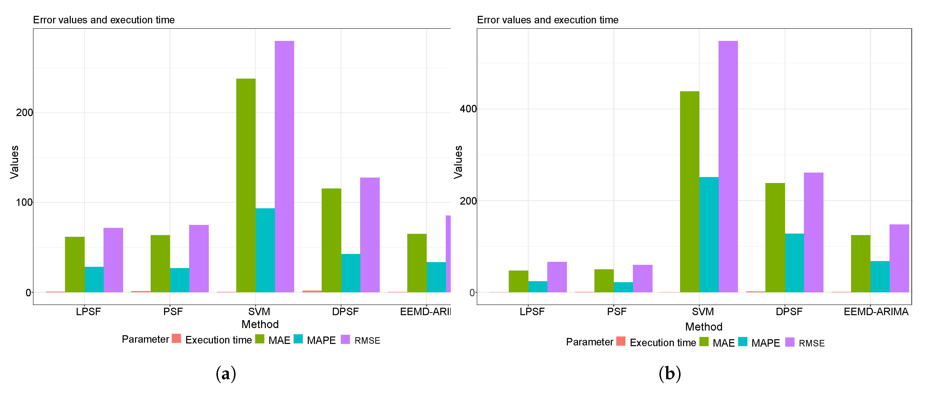
4. Case Study Related to the Energy Application

In the current research, it is important to validate the proposed R package ForecastTB based on real-world applications. In this manner, a reliable and feasible application can demonstrate the capacity of the developed R package forecasting code. Wind speed and solar radiation data of two meteorological stations (Robinson and Watford City) located in the North Dakota, USA, were used to test the predictability performance of the LPSF: modified pattern sequence-based forecast and PSF—pattern sequence-based forecast models. Three time scales were examined for the forecasting of 12 steps ahead of each scale including daily, weekly, and monthly. The modeling result was tested using several statistical performance metrics (RMSE, MAE, and MAPE), time convergence, and graphical presentation. The data span covers 20 years of historical data over the period (1 January 2000 to 31 December 2019). Three models were developed for modeling verification including support vector machine (SVM), decomposed pattern sequence-based forecast (DPSF), and hybridized ensemble empirical mode decomposition with Autoregressive integrated moving average (EEMD-ARIMA).

4.1. Statistical Performance Metrics Results

Following several established studies from the literature on wind speed and solar radiation prediction, RMSE, MAE, and MAPE are the commonly used statistical metrics for forecasting evaluation [48]. Those metrics can give an informative evaluation of the prediction capacity. For the Robinson station, the forecasting results attained the minimal values of the absolute error measures for the applied models—LPSF (RMSE = 7.57 and 71.6, MAE = 5.34 and 61.52 and MAPE = 35.84 and 28.22) and PSF (RMSE = 8.47 and 74.74, MAE = 7.0 and 63.65 and MAPE = 57.69 and 26.93) for the daily scale wind speed and solar radiation; LPSF (RMSE = 3.75 and 66.17, MAE = 3.2 and 47.36 and MAPE = 32.82 and 23.72) and PSF (RMSE = 3.3 and 59.33, MAE = 3.57 and 49.72 and MAPE = 24.5 and 21.88) for the weekly scale wind speed and solar radiation; LPSF (RMSE = 2.09 and 99.8, MAE = 1.58 and 82.74 and MAPE = 19.15 and 33.79) and PSF (RMSE = 1.6 and 39.32, MAE = 1.19 and 32.51 and MAPE = 13.77 and 10.84) for the monthly scale wind speed and solar radiation, respectively (

Table 1. The statistical performance of the forecasting wind speed and solar radiation at Robinson station for the daily, weekly and monthly time scale for the applied (LSPF and PSF) and the comparable predictive models (i.e., SVM, DPSF and EEMD-ARIMA).

Methods	Wind Speed				Solar Radiation
Daily Scale
	RMSE	MAE	MAPE	Execution Time	RMSE	MAE	MAPE	Execution Time
LPSF	7.57	5.34	35.84	0.55	71.60	61.52	28.22	0.49
PSF	8.47	7.00	57.69	0.42	74.74	63.65	26.93	1.06
SVM	54.28	49.02	472.57	0.43	279.86	237.87	93.45	0.30
DPSF	13.24	11.07	73.07	1.12	127.47	115.48	42.43	1.63
EEMD-ARIMA	9.38	7.99	74.56	0.25	85.32	64.96	33.35	0.23
Weekly Scale
	RMSE	MAE	MAPE	Execution Time	RMSE	MAE	MAPE	Execution Time
LPSF	3.75	3.20	32.82	0.19	66.17	47.36	23.72	0.30
PSF	3.30	2.57	24.50	0.50	59.33	49.72	21.88	0.78
SVM	13.51	10.73	117.89	0.30	548.47	438.63	250.93	0.24
DPSF	3.40	2.74	24.28	1.64	260.68	238.28	128.00	1.77
EEMD-ARIMA	2.73	2.33	24.60	0.44	147.88	124.65	67.65	0.39
Monthly Scale
	RMSE	MAE	MAPE	Execution Time	RMSE	MAE	MAPE	Execution Time
LPSF	2.09	1.58	19.15	0.47	99.80	82.74	33.79	0.46
PSF	1.60	1.19	13.77	0.35	39.32	32.51	10.84	0.32
SVM	8.66	7.11	77.86	0.18	3881.20	3384.89	1632.05	0.19
DPSF	1.73	1.49	16.65	0.95	100.60	88.72	32.25	1.02
EEMD-ARIMA	1.93	1.63	19.55	0.19	50.00	36.94	13.90	3.62

). In comparison with the SVM, DPSF and EEMD-ARIMA, the LPSF and PSF models revealed an acceptable prediction enhancement. For instance, wind speed prediction was improved using the LPSF model by (86.04%, 42.77%, and 19.22%) based on the RMSE metric against the SVM, DPSF, and EEMD-ARIMA models, respectively. Whereas, solar radiation prediction accuracy was enhanced by (74.41%, 43.83% and 16.08%) using the LPSF model and RMSE metric over the SVM, DPSF and EEMD-ARIMA models, respectively.

For Watford City station, the best forecasting results achieved for the proposed LPSF and PSF models with minimum values of (RMSE, MAE, and MAPE). Statistically, the performance metrics accomplished were; LPSF (RMSE = 6.67 and 162.74, MAE = 5.48 and 158.21 and MAPE = 39.85 and 156.09) and PSF (RMSE = 6.98 and 131.67, MAE = 5.73 and 123.64 and MAPE = 41.45 and 125.34) for the daily scale wind speed and solar radiation; LPSF (RMSE = 2.95 and 70.21, MAE = 2.04 and 55.65 and MAPE = 23.68 and 26.74) and PSF (RMSE = 2.18 and 80.83, MAE = 1.79 and 68.79 and MAPE = 21.33 and 32.76) for the weekly scale wind speed and solar radiation; LPSF (RMSE = 1.98 and 115.18, MAE = 1.7 and 90.65 and MAPE = 20.16 and 42.48) and PSF (RMSE = 1.43 and 32.09, MAE = 1.17 and 25.23 and MAPE = 13.84 and 8.77) for the monthly scale wind speed and solar radiation, respectively (

Table 2. The statistical performance of the forecasting wind speed and solar radiation at Watford City station for the daily, weekly and monthly time scale for the applied (LSPF and PSF) and the comparable predictive models (i.e., SVM, DPSF and EEMD-ARIMA).

Methods	Wind Speed				Solar Radiation
Daily Scale
	RMSE	MAE	MAPE	Execution Time	RMSE	MAE	MAPE	Execution Time
LPSF	6.67	5.48	39.85	0.48	162.74	158.21	156.09	0.23
PSF	6.98	5.73	41.45	0.67	131.67	123.64	125.34	1.69
SVM	39.51	36.36	377.76	0.26	235.05	198.34	192.34	0.26
DPSF	10.48	9.02	64.90	1.77	44.29	36.30	30.20	1.18
EEMD-ARIMA	9.20	8.20	64.60	0.27	33.86	29.13	29.67	0.54
Weekly Scale
	RMSE	MAE	MAPE	Execution Time	RMSE	MAE	MAPE	Execution Time
LPSF	2.95	2.04	23.68	0.79	70.21	55.65	26.74	0.22
PSF	2.18	1.79	21.33	0.44	80.83	68.79	32.76	0.96
SVM	11.05	8.60	94.95	0.26	117.46	89.32	53.93	0.53
DPSF	2.28	1.61	17.26	2.16	134.15	124.54	61.43	1.21
EEMD-ARIMA	1.87	1.55	17.56	0.38	147.10	126.24	71.94	0.23
Monthly Scale
	RMSE	MAE	MAPE	Execution Time	RMSE	MAE	MAPE	Execution Time
LPSF	1.98	1.70	20.16	1.30	115.18	90.65	42.48	1.05
PSF	1.43	1.17	13.84	0.71	32.09	25.23	8.77	0.49
SVM	3.34	2.74	31.63	0.37	3739.78	3231.79	1719.36	0.52
DPSF	1.90	1.67	19.46	1.79	102.93	92,20	35.60	1.76
EEMD-ARIMA	1.30	1.02	11.29	0.73	65.96	58.27	26.29	0.39

). The statistical results of the Watford City station demonstrated more or less similar predictability performance of wind speed and solar radiation in comparison with the benchmark models (i.e., SVM, DPSF and EEMD-ARIMA).

The convergence execution time is one of the essential modeling components in the field of soft computing and modeling aspects [49]. With respect to the convergence execution time of the developed models, the LPSF and PSF revealed a very faster time learning process with an acceptable execution process.

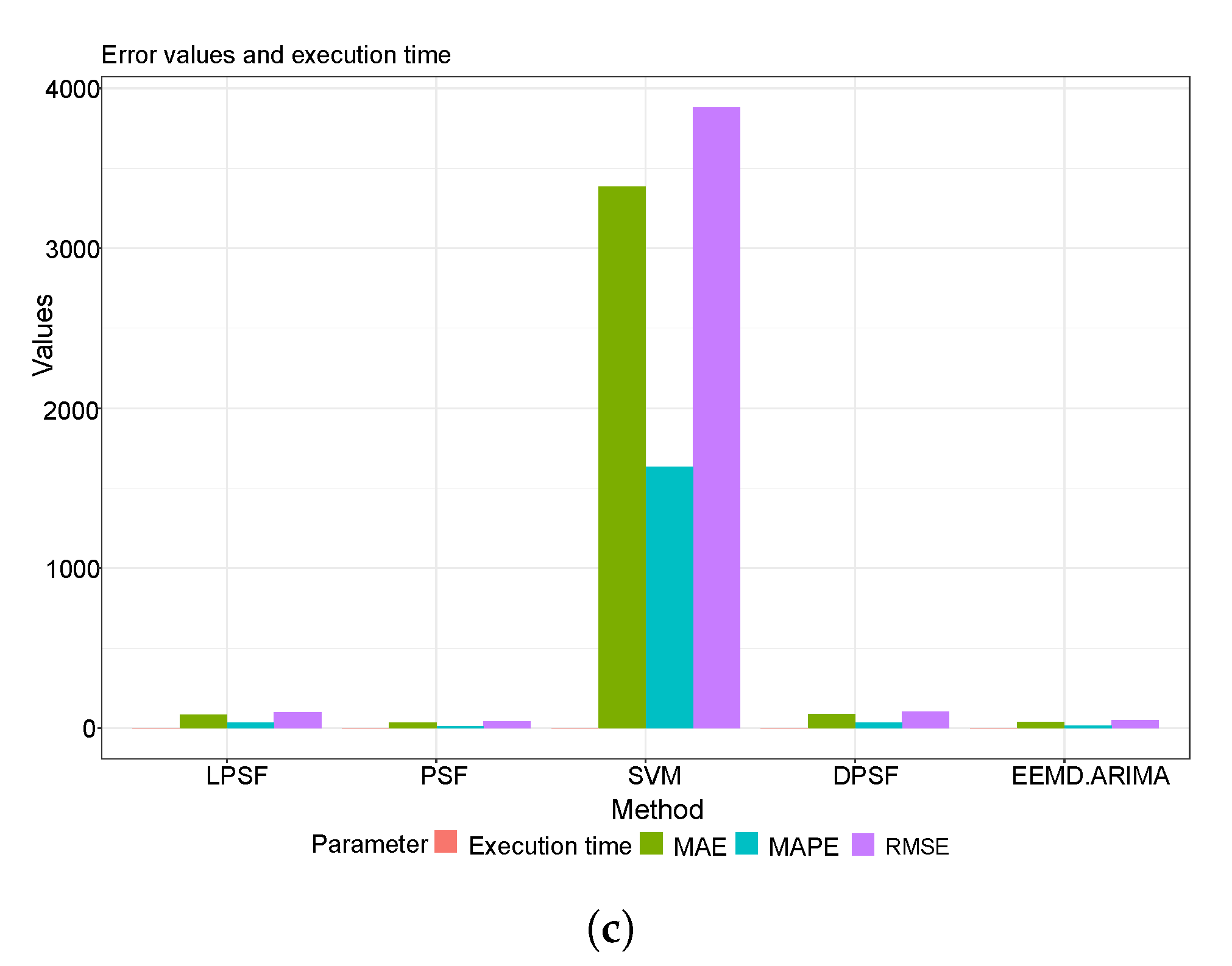
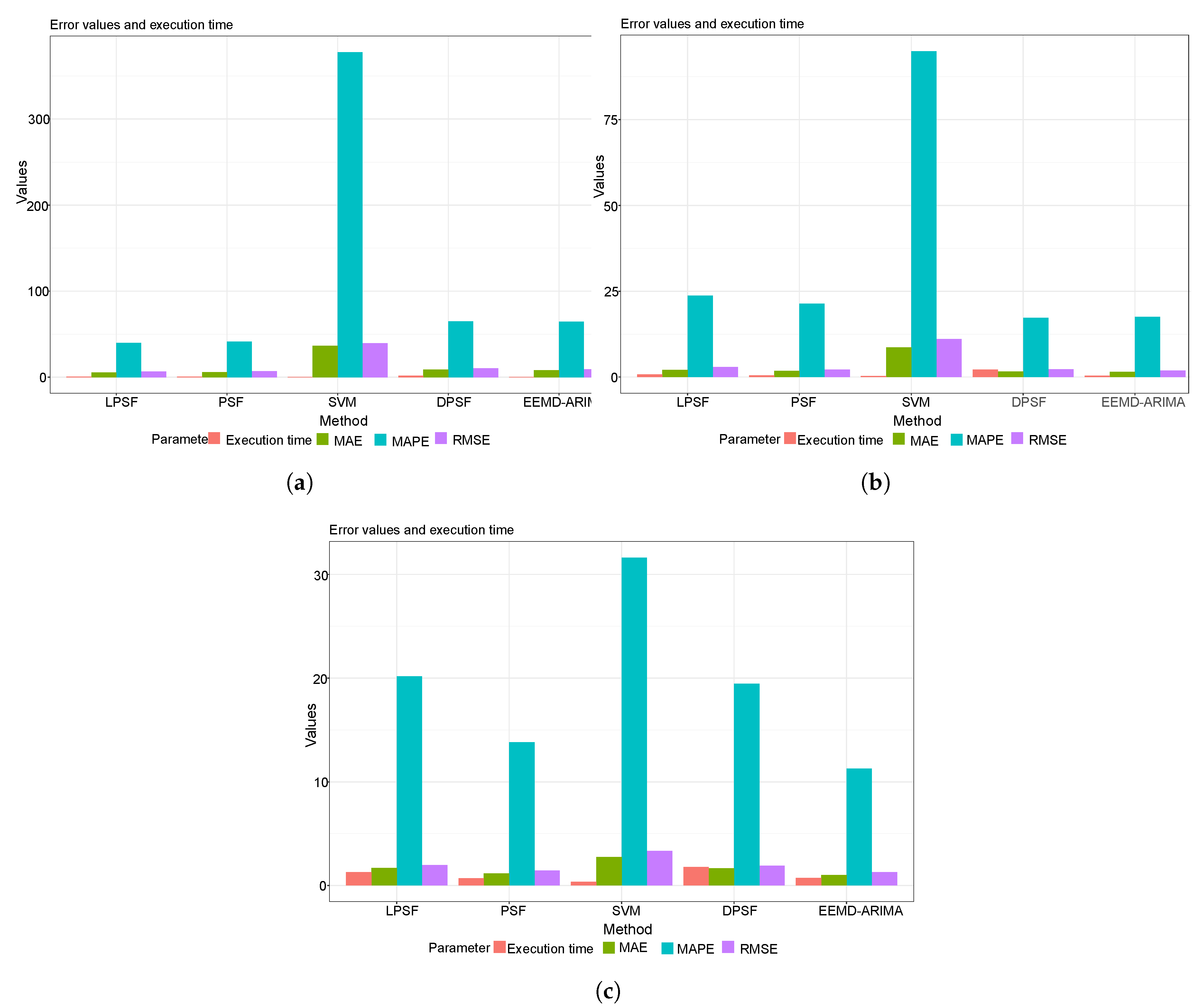
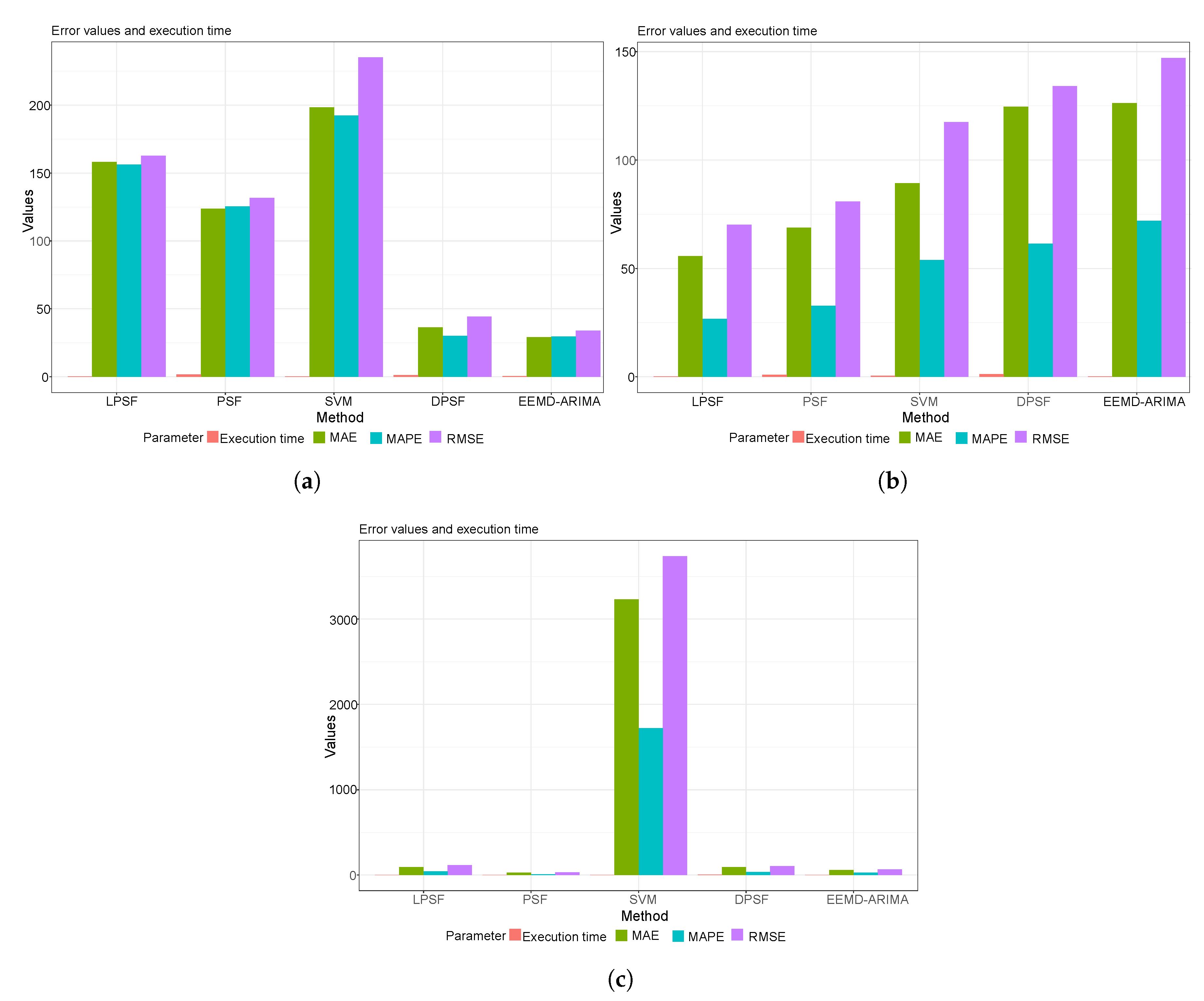
4.2. The Graphical Presentation of the Developed Forecasting Models

Figure 5a–c reported the performance metrics and time execution results of the wind speed forecasting daily, weekly, and monthly in the form of a bar chart. For all investigated time scales, the LPSF and PSF models revealed a slightly similar performance to the DPSF and EEMD-ARIMA. However, the SVM model showed very poor predictability performance and this can be explained due to the essential tuning procedure required for the SVM model for the internal parameters, that were not adopted or focused on in this research [50,51]. Figure 6a–c indicated the performance metrics and time execution results of solar radiation forecasting for the daily, weekly, and monthly scales at the Robinson station. It is clearly seen that the monthly scale solar radiation for LPSF, PSF, DPSF, and EEMD-ARIMA models were similar. However, the SVM model still reported the lowest capacity. Figure 7a–c displayed the forecasting capacity of the proposed and comparable forecasting models for wind speed modeling at Watford City station. For the daily and weekly wind speed scales, the LPSF and PSF models exhibited a distinguished performance against the results of SVM models. Yet, the monthly scale results of the LPSF, and PSF models were slightly poorer and similar to the ones attained by DPSF and EEMD-ARIMA. Figure 8a–c reported the performance of the solar radiation forecasting Watford City station and for all molded time series scales. For the daily scale, Figure 8a shows that the performance of the DPSF and EEMD-ARIMA models is superior to that of the LPSF models and PSF models. This might be due to the high stochasticity of the solar radiation process on a daily scale and thus the proposed models could not capture the actual trend. On the weekly base scale, the DPSF and EEMD-ARIMA models indicated the worst forecasting potential, even worse than the SVM model. Whereas, similar performance attained using LPSF, PSF, DPSF, and EEMD-ARIMA models for the monthly scale of solar radiation other hand, for the monthly.

5. Discussion

This article proposed and demonstrated the ForecastTB package as a test-bench for comparing the time series forecasting methods as a crucial step towards more formal time series analysis. This demonstration is further described with some case studies to show how characteristics of the temporal correlation structure can influence the forecast accuracy. The ForecastTB package greatly assists in comparing different forecasting methods and considering the characteristic of the time series dataset.

Also, this paper explains how new forecasting methods and error metrics can be introduced in the comparative test-bench. As such, the package allows users to include additional forecasting methods for comparison, which can be extremely useful given the capability of R to interface with other programming languages (e.g., matlabr for MatLab [52]; Rcpp for compiled languages [53] and many other). Finally, a simple plug-and-play module based architecture of the ForecastTB to append or remove several forecasting methods and error metrics makes it a robust and handy tool to evaluate forecasting analysis.

It is worth mentioning that forecasting different time scale wind speed and solar radiation is highly essential for multiple energy sources harvesting [54,55,56]. Providing an accurate and reliable forecasting intelligent computer aid models for wind speed and solar radiation can contribute to the base knowledge of friendly energy sources and sustainable green cities. To the best knowledge of the current research, the feasibility of the LPSF and PSF models is evidenced to be capable to module related energy datasets.

References

1. Sagheer, A.; Kotb, M. Time series forecasting of petroleum production using deep LSTM recurrent networks. Neurocomputing 2019, 323, 203–213. [Google Scholar] [CrossRef]
2. Bokde, N.; Feijóo, A.; Kulat, K. Analysis of differencing and decomposition preprocessing methods for wind speed prediction. Appl. Soft Comput. 2018, 71, 926–938. [Google Scholar] [CrossRef]
3. Arce, P.; Antognini, J.; Kristjanpoller, W.; Salinas, L. Fast and Adaptive Cointegration Based Model for Forecasting High Frequency Financial Time Series. Comput. Econ. 2019, 54, 99–112. [Google Scholar] [CrossRef]
4. Gonzalez-Vidal, A.; Jimenez, F.; Gomez-Skarmeta, A.F. A methodology for energy multivariate time series forecasting in smart buildings based on feature selection. Energy Build. 2019, 196, 71–82. [Google Scholar] [CrossRef]
5. Divina, F.; García Torres, M.; Goméz Vela, F.A.; Vázquez Noguera, J.L. A comparative study of time series forecasting methods for short term electric energy consumption prediction in smart buildings. Energies 2019, 12, 1934. [Google Scholar] [CrossRef] [Green Version]
6. Shih, H.; Rajendran, S. Comparison of time series methods and machine learning algorithms for forecasting Taiwan Blood Services Foundation’s blood supply. J. Healthc. Eng. 2019, 2019, 6123745. [Google Scholar] [CrossRef]
7. Vázquez, M.; Melin, P.; Prado-Arechiga, G. Hybrid Neural-Fuzzy Modeling and Classification System for Blood Pressure Level Affectation. In Hybrid Intelligent Systems in Control, Pattern Recognition and Medicine; Springer: Berlin/Heidelberg, Germany, 2020; pp. 257–269. [Google Scholar]
8. Mithiya, D.; Datta, L.; Mandal, K. Time Series Analysis and Forecasting of Oilseeds Production in India: Using Autoregressive Integrated Moving Average and Group Method of Data Handling–Neural Network. Asian J. Agric. Ext. Econ. Sociol. 2019, 30, 1–14. [Google Scholar] [CrossRef] [Green Version]
9. Gupta, A.; Bokde, N.; Kulat, K. Hybrid leakage management for water network using PSF algorithm and soft computing techniques. Water Resour. Manag. 2018, 32, 1133–1151. [Google Scholar] [CrossRef]
10. Kim, J.; Lee, H. A study on predictive model for forecasting anti-aircraft missile spare parts demand based on machine learning. Korean Data Inf. Sci. Soc. 2019, 30, 587–596. [Google Scholar]
11. Eze, N.; Asogwa, O.; Obetta, A.; Ojide, K.; Okonkwo, C. A Time Series Analysis of Federal Budgetary Allocations to Education Sector in Nigeria (1970–2018). Am. J. Appl. Math. Stat. 2020, 8, 1–8. [Google Scholar]
12. Li, M.; Hinnov, L.; Kump, L. Acycle: Time-series analysis software for paleoclimate research and education. Comput. Geosci. 2019, 127, 12–22. [Google Scholar] [CrossRef]
13. Adamuthe, A.C.; Thampi, G.T. Technology forecasting: A case study of computational technologies. Technol. Forecast. Soc. Chang. 2019, 143, 181–189. [Google Scholar] [CrossRef]
14. Patil, J.; Bokde, N.; Mishra, S.K.; Kulat, K. PSF-Based Spectrum Occupancy Prediction in Cognitive Radio. In Advanced Engineering Optimization Through Intelligent Techniques; Springer: Berlin/Heidelberg, Germany, 2020; pp. 609–619. [Google Scholar]
15. Maroufpoor, S.; Maroufpoor, E.; Bozorg-Haddad, O.; Shiri, J.; Yaseen, Z.M. Soil moisture simulation using hybrid artificial intelligent model: Hybridization of adaptive neuro fuzzy inference system with grey wolf optimizer algorithm. J. Hydrol. 2019, 575, 544–556. [Google Scholar] [CrossRef]
16. Sanikhani, H.; Deo, R.C.; Samui, P.; Kisi, O.; Mert, C.; Mirabbasi, R.; Gavili, S.; Yaseen, Z.M. Survey of different data-intelligent modeling strategies for forecasting air temperature using geographic information as model predictors. Comput. Electron. Agric. 2018, 152, 242–260. [Google Scholar] [CrossRef]
17. Yaseen, Z.M.; Tran, M.T.; Kim, S.; Bakhshpoori, T.; Deo, R.C. Shear strength prediction of steel fiber reinforced concrete beam using hybrid intelligence models: A new approach. Eng. Struct. 2018, 177, 244–255. [Google Scholar] [CrossRef]
18. Casdagli, M. Chaos and deterministic versus stochastic non-linear modelling. J. R. Stat. Soc. Ser. B (Methodol.) 1992, 54, 303–328. [Google Scholar]
19. Shumway, R.H.; Stoffer, D.S. Time series analysis and its applications. Stud. Inform. Control 2000, 9, 375–376. [Google Scholar]
20. Box, G.E.; Jenkins, G.M.; Reinsel, G.C.; Ljung, G.M. Time Series Analysis: Forecasting and Control; John Wiley & Sons: Hoboken, NJ, USA, 2015. [Google Scholar]
21. Yaseen, Z.M.; Mohtar, W.H.M.W.; Ameen, A.M.S.; Ebtehaj, I.; Razali, S.F.M.; Bonakdari, H.; Salih, S.Q.; Al-Ansari, N.; Shahid, S. Implementation of univariate paradigm for streamflow simulation using hybrid data-driven model: Case study in tropical region. IEEE Access 2019, 7, 74471–74481. [Google Scholar] [CrossRef]
22. Beyaztas, U.; Salih, S.Q.; Chau, K.W.; Al-Ansari, N.; Yaseen, Z.M. Construction of functional data analysis modeling strategy for global solar radiation prediction: Application of cross-station paradigm. Eng. Appl. Comput. Fluid Mech. 2019, 13, 1165–1181. [Google Scholar] [CrossRef]
23. Yozgatligil, C.; Aslan, S.; Iyigun, C.; Batmaz, I. Comparison of missing value imputation methods in time series: The case of Turkish meteorological data. Theor. Appl. Climatol. 2013, 112, 143–167. [Google Scholar] [CrossRef]
24. Tao, H.; Salih, S.Q.; Saggi, M.K.; Dodangeh, E.; Voyant, C.; Al-Ansari, N.; Yaseen, Z.M.; Shahid, S. A Newly Developed Integrative Bio-Inspired Artificial Intelligence Model for Wind Speed Prediction. IEEE Access 2020, 8, 83347–83358. [Google Scholar] [CrossRef]
25. Bokde, N.D.; Andersen, G.B. ForecastTB: Test Bench for the Comparison of Forecast Methods; R Package Version 1.0.1; R Foundation for Statistical Computing: Vienna, Austria, 2020. [Google Scholar]
26. Beck, M.W.; Bokde, N.; Asencio-Cortés, G.; Kulat, K. R package imputetestbench to compare imputation methods for univariate time series. R J. 2018, 10, 218. [Google Scholar] [CrossRef] [PubMed] [Green Version]
27. Bokde, N.; Beck, M. imputeTestbench: Test Bench for Missing Data Imputing Models/Methods Comparison; R Package Version 3.0.3; R Foundation for Statistical Computing: Vienna, Austria, 2016. [Google Scholar]
28. Bokde, N.; Beck, M.W.; Álvarez, F.M.; Kulat, K. A novel imputation methodology for time series based on pattern sequence forecasting. Pattern Recognit. Lett. 2018, 116, 88–96. [Google Scholar] [CrossRef] [PubMed]
29. Shaadan, N.; Rahim, N. Imputation Analysis for Time Series Air Quality (PM10) Data Set: A Comparison of Several Methods. J. Phys. Conf. Ser. Iop Publ. 2019, 1366, 012107. [Google Scholar] [CrossRef]
30. Arowolo, O.A. Foreign Investment Dependence and Infant Mortality Outcomes in the Sub-Sahara: A Bayesian P-Spline Approach to Processing Missing Sub-Regional Data. Ph.D. Thesis, University of Texas, Dallas, TX, USA, 2019. [Google Scholar]
31. Bokde, N.; Feijóo, A.; Villanueva, D. Wind Turbine Power Curves Based on the Weibull Cumulative Distribution Function. Appl. Sci. 2018, 8, 1757. [Google Scholar] [CrossRef] [Green Version]
32. Wickham, H. Reshaping Data with the reshape Package. J. Stat. Softw. 2007, 21, 1–20. [Google Scholar] [CrossRef]
33. R Core Team. R: A Language and Environment for Statistical Computing; R Foundation for Statistical Computing: Vienna, Austria, 2019. [Google Scholar]
34. Wickham, H. ggplot2: Elegant Graphics for Data Analysis; Springer: New York, NY, USA, 2016. [Google Scholar]
35. Gu, Z.; Gu, L.; Eils, R.; Schlesner, M.; Brors, B. circlize implements and enhances circular visualization in R. Bioinformatics 2014, 30, 2811–2812. [Google Scholar] [CrossRef] [Green Version]
36. Auguie, B. gridExtra: Miscellaneous Functions for “Grid” Graphics; R Package Version 2.3; R Foundation for Statistical Computing: Vienna, Austria, 2017. [Google Scholar]
37. Neuwirth, E. RColorBrewer: ColorBrewer Palettes; R Package Version 1.1-2; R Foundation for Statistical Computing: Vienna, Austria , 2014. [Google Scholar]
38. Hyndman, R.J.; Khandakar, Y. Automatic time series forecasting: The forecast package for R. J. Stat. Softw. 2008, 26, 1–22. [Google Scholar]
39. Bokde, N.; Asencio-Cortes, G.; Martinez-Alvarez, F. PSF: Forecasting of Univariate Time Series Using the Pattern Sequence-Based Forecasting (PSF) Algorithm; R Package Version 0.4; R Foundation for Statistical Computing: Vienna, Austria, 2017. [Google Scholar]
40. Bokde, N.; Asencio-Cortés, G.; Martínez-Álvarez, F.; Kulat, K. PSF: Introduction to R Package for Pattern Sequence Based Forecasting Algorithm. R J. 2017, 9, 324–333. [Google Scholar] [CrossRef] [Green Version]
41. Alvarez, F.M.; Troncoso, A.; Riquelme, J.C.; Ruiz, J.S.A. Energy time series forecasting based on pattern sequence similarity. IEEE Trans. Knowl. Data Eng. 2010, 23, 1230–1243. [Google Scholar] [CrossRef]
42. Bokde, N. decomposedPSF: Time Series Prediction with PSF and Decomposition Methods (EMD and EEMD); R Package Version 0.1.3; R Foundation for Statistical Computing: Vienna, Austria, 2017. [Google Scholar]
43. Vico Moreno, A.; Rivera Rivas, A.J.; Perez Godoy, M.D. PredtoolsTS: Time Series Prediction Tools; R Package Version 0.1.1; R Foundation for Statistical Computing: Vienna, Austria, 2018. [Google Scholar]
44. Charte, F.; Vico, A.; Pérez-Godoy, M.D.; Rivera, A.J. predtoolsTS: R package for streamlining time series forecasting. Prog. Artif. Intell. 2019, 8, 505–510. [Google Scholar] [CrossRef]
45. Kuhn, M. Caret: Classification and Regression Training; R Package Version 6.0-85; R Foundation for Statistical Computing: Vienna, Austria, 2020. [Google Scholar]
46. Sharafati, A.; Khosravi, K.; Khosravinia, P.; Ahmed, K.; Salman, S.A.; Yaseen, Z.M.; Shahid, S. The potential of novel data mining models for global solar radiation prediction. Int. J. Environ. Sci. Technol. 2019, 16, 7147–7164. [Google Scholar] [CrossRef]
47. Tak, S.; Woo, S.; Yeo, H. Data-driven imputation method for traffic data in sectional units of road links. IEEE Trans. Intell. Transp. Syst. 2016, 17, 1762–1771. [Google Scholar] [CrossRef]
48. Elsheikh, A.H.; Sharshir, S.W.; Elaziz, M.A.; Kabeel, A.; Guilan, W.; Haiou, Z. Modeling of solar energy systems using artificial neural network: A comprehensive review. Sol. Energy 2019, 180, 622–639. [Google Scholar] [CrossRef]
49. Yaseen, Z.M.; Sulaiman, S.O.; Deo, R.C.; Chau, K.W. An enhanced extreme learning machine model for river flow forecasting: State-of-the-art, practical applications in water resource engineering area and future research direction. J. Hydrol. 2019, 569, 387–408. [Google Scholar] [CrossRef]
50. Al-Musawi, A.A.; Alwanas, A.A.; Salih, S.Q.; Ali, Z.H.; Tran, M.T.; Yaseen, Z.M. Shear strength of SFRCB without stirrups simulation: Implementation of hybrid artificial intelligence model. Eng. Comput. 2020, 36, 1–11. [Google Scholar] [CrossRef]
51. Tao, H.; Sulaiman, S.O.; Yaseen, Z.M.; Asadi, H.; Meshram, S.G.; Ghorbani, M. What is the potential of integrating phase space reconstruction with SVM-FFA data-intelligence model? Application of rainfall forecasting over regional scale. Water Resour. Manag. 2018, 32, 3935–3959. [Google Scholar] [CrossRef]
52. Muschelli, J. Matlabr: An Interface for MATLAB using System Calls; R Package Version 1.5.2; R Foundation for Statistical Computing: Vienna, Austria, 2018. [Google Scholar]
53. Eddelbuettel, D.; François, R.; Allaire, J.; Ushey, K.; Kou, Q.; Russel, N.; Chambers, J.; Bates, D. Rcpp: Seamless R and C++ integration. J. Stat. Softw. 2011, 40, 1–18. [Google Scholar] [CrossRef] [Green Version]
54. Kisi, O.; Heddam, S.; Yaseen, Z.M. The implementation of univariable scheme-based air temperature for solar radiation prediction: New development of dynamic evolving neural-fuzzy inference system model. Appl. Energy 2019, 241, 184–195. [Google Scholar] [CrossRef]
55. Tao, H.; Ebtehaj, I.; Bonakdari, H.; Heddam, S.; Voyant, C.; Al-Ansari, N.; Deo, R.; Yaseen, Z.M. Designing a new data intelligence model for global solar radiation prediction: Application of multivariate modeling scheme. Energies 2019, 12, 1365. [Google Scholar] [CrossRef] [Green Version]
56. Bokde, N.; Feijóo, A.; Villanueva, D.; Kulat, K. A review on hybrid empirical mode decomposition models for wind speed and wind power prediction. Energies 2019, 12, 254. [Google Scholar] [CrossRef] [Green Version]
Figure 1. The plug-and-play module of the ForecastTB package.
Energies 13 02578 g001
Figure 2. Forecasting errors (in bar plot) and forecasted values (in line plot) for methods attached in the object c1.
Energies 13 02578 g002
Figure 3. A plot showing the new error function in prediction_errors object.
Energies 13 02578 g003
Figure 4. A polar plot to represent forecasted values.
Energies 13 02578 g004
Figure 5. The bar chart of the performance metrics and time execution results of wind speed forecasting for the daily (a), weekly (b) and monthly (c) at Robinson station.
Energies 13 02578 g005
Figure 6. The bar chart of the performance metrics and time execution results of solar radiation forecasting for the daily (a), weekly (b) and monthly (c) at Robinson station.
Energies 13 02578 g006aEnergies 13 02578 g006b
Figure 7. The bar chart of the performance metrics and time execution results of wind speed forecasting for the daily (a), weekly (b) and monthly (c) at Watford City station.
Energies 13 02578 g007
Figure 8. The bar chart of the performance metrics and time execution results of solar radiation forecasting for the daily (a), weekly (b) and monthly (c) at Watford City station.
Energies 13 02578 g008