Abstract
Increased concerns over global warming and air pollution has pushed governments to consider renewable energy as an alternative to meet the required energy demands of countries. Many government policies are deployed in Taiwan to promote solar and wind energy to cope with air pollution and self-dependency for energy generation. However, the residential sector contribution is not significant despite higher feed-in tariff rates set by government. This study analyzes wind and solar power availability of four different locations of southern Taiwan, based on the Köppen–Geiger climate classification system. The solar–wind hybrid system (SWHS) considered in this study consists of multi-crystalline photovoltaic (PV) modules, vertical wind turbines, inverters and batteries. Global reanalysis weather data and a climate-based electricity load profile at a 1-h resolution was used for the simulation. A general framework for multi-objective optimization using this simulation technique is proposed for solar–wind hybrid system, considering the feed-in tariff regulations, environmental regulations and installation area constraints of Taiwan. The hourly load profile is selected using a climate classification system. A decomposition-based differential evolutionary algorithm is used for finding the optimal Pareto set of two economic objectives and one environmental objective with maximum installation area and maximum PV capacity constraints. Two types of buildings are chosen for analysis at four climate locations. Analysis of Pareto sets revealed that the photovoltaic modules are economic options for a grid-connected mode at all four locations, whereas solar–wind hybrid systems are more environmentally friendly. A method of finding the fitness index for the Pareto front sets and a balanced strategy for choosing the optimal configuration is proposed. The proposed balanced strategy provides savings to users—up to 49% for urban residential buildings and up to 32% for rural residential buildings with respect to buildings without a hybrid energy system (HES)—while keeping carbon dioxide (CO2) emissions lower than 50% for the total project lifecycle time of 20 years. The case study reveals that for all four locations and two building types an HES system comprising a 15 kW photovoltaic system and a small capacity battery bank provides the optimal balance between economic and environmental objectives.
1. Introduction
Global warming is one of the biggest concerns among global communities [1,2]. The climate action summit [3] organized by the United Nations (UN) in 2019 set a goal of achieving a 1.5 °C goal by the end of the century, by reducing GHG emissions by 7.6% annually. The target includes decreasing the dependency on fossil fuels and promoting clean energy. According to the International Renewable Energy Agency (IRENA), Asia would continue to dominate the solar photovoltaic (PV) [4] and onshore wind [5] power industries with an estimated share of more than 50% in both sectors by 2050. Taiwan has implemented several policies to promote renewable energy generation. The million solar rooftop PVs project [6,7] focuses on the gradual expansion of rooftop PV installation prior to ground installations, and the thousand wind turbine project proposes the strategy of developing onshore wind power systems before off-shore wind farms. Furthermore, the Bureau of Energy has announced promotional feed-in tariff (FiT) rates [8] for onshore wind power with capacity between 1 kW and 30 kW and rooftop solar PV systems with capacities between 1 kW and 20 kW. The “Greenhouse Gas Reduction and Management Act” [9,10] enacted by Taiwan, legislates a 50% reduction target for 2050 compared to 2005 levels. This act also implements carbon reduction by setting goals every five years. The Environmental Protection Administration (EPA), Taiwan, also encourages and develops strategies to build low-carbon infrastructures for local communities.
Government incentives and FiT play important roles in designing and sizing of hybrid power system. Economic factors, such as net present cost (NPC), levelized cost of energy (LCOE) and total cost of power bought from the grid over the project lifecycle time, have great impact on the choices made by independent electricity users. The environmental objective of such systems mainly focuses on reducing overall GHG emissions (CO2 emission in particular). Many studies have proposed sizing optimization methods and strategies for hybrid energy systems [11,12]. Optimal sizing of a hybrid renewable energy system (HRES), considering the economic objectives like NPC, initial capital and system payback period, are discussed in detail in [13,14]. Weather and energy price data are important for hybrid energy system (HES) cost optimization. Using this concept, a quantitative control approach to reduce the HES energy cost is proposed by [15]. The clear advantages of multi-objective optimization using meta-heuristics approaches as opposed to the iterative method and linear programming is discussed in [16]. Many multi-objective approaches for HES optimization have also been proposed over the years, considering several criteria, including technical, economic, environmental and socio-political objectives [17,18,19,20].
Several meta-heuristic algorithms have been developed by researchers for handling multi-objective optimization problems. The two widely used multi-objective optimization algorithms are the non-dominated sorting genetic algorithm (NSGA-II) [21] and the multi-objective evolutionary algorithm based on decomposition (MOEA/D) [22]. The solar–wind hybrid power generation optimization method proposed in [23], hybrid distributed energy system (HDES) optimization presented in [24] as well as the hydro–PV HES optimization [25] uses NSGA-II for finding the optimal Pareto sets. The goal of optimal sizing for an HES or HRES is to find the optimal configuration of the components of the system based on multi-objective Pareto set analysis. In [26], the differential evolution variant of MOEA/D (MOEA/D-DE) is used for multi-objective optimization of an off-grid solar/wind/battery HES. MOEA/D and MOEA/D-DE are frequently used in engineering optimization problems [27,28,29,30]. An enhanced MOEA/D using a localized penalty-based boundary intersection is proposed in [31] for HRES optimization. Power optimization of HRES with the help of neural architecture and the bee colony algorithm is presented as an alternative to traditional optimization methods in [32]. A combined dispatch strategy for HES optimization and energy management is proposed in [33]. This study shows that a combined dispatch strategy can reduce the NPC, cost of electricity and CO2 emissions. Several multi-objective optimization algorithms and methods have been studied for the HRES and microgrid sizing that either focus on advanced algorithms [34,35] or dealing with optimization uncertainties [36]. Several commercial HES and microgrid optimization tools use mono-objective optimization or a linearized model for optimization. In [37], the authors developed a multi-objective optimization tool for HRES configurations. An HES with renewable energy and a hydrogen generation system is optimized in [38], using typical load profiles and historic weather data.
Some studies have tried to study the effect of climate on energy requirement and production. In [39], the authors have presented a methodology for a PV climate classification and studied the climate’s implication for PV system performance. Similarly, in [40] a database is presented for promoting a ground source heat pump by studying the climate data of Europe using the Köppen–Geiger scale. Reference [41] introduces a multi-criteria decision-making method for an HRES system. This study also briefly introduces other studies targeting different climate areas. The system design as well as the feasibility of the trigeneration systems for zero-energy office buildings in three climate areas, Stuttgart, Dubai and Moscow, are discussed in [42]. A location’s climate condition for stand-alone HES optimization is taken into account in [43].
Most of the studies mentioned above uses typical load and weather profiles. Several times, these profiles are artificially modeled and may not represent the real-world conditions. The residential buildings in Taiwan are constraint by installation area limits due to higher property prices and a high population density. Therefore, the feasibility of an HES system for residential buildings are explored using case study analysis. In this study, we also try to overcome the unavailability of the hourly load-profile data of the Taiwan region by using alternative profiles from similar climate zones. We also propose a framework to optimize and analyze the multiple objectives of a solar–wind HES system by considering the different socio-political and economical factor of the Taiwan region. In summary:
- This study proposes a general framework for multi-objective optimization of the NPC, total power bought from the grid and total CO2 emission objectives for a project lifecycle of 20 years. The power trading method includes different FiT rates for solar and wind power, as stated by the local government. Climate classification scales are used to obtain the hourly load profiles. Maximum solar power and installation area constraints are used.
- A fitness evaluation method with a balanced selection strategy is introduced for Pareto optimal sets to maximize the savings from the HES system while keeping the CO2 emissions at least 50% lower than the “No-HES” systems.
- The results of the case study show that by using the proposed balanced strategy to select a balanced HES configuration, residential building users can save up to 49% in urban building areas and up to 32% in rural buildings.
- The case study shows that wind power is crucial for reducing the total CO2 emissions and reducing the dependability on the utility grid while being constrained by a limited installation area. However, the higher NPC rates makes it non-feasible for independent electricity users to use wind power without government incentives.
- The case study also shows that an HES system consisting of a 15 kW PV system and small capacity battery bank provides the optimal balance between the economic and environmental objectives.
We organized the paper as follows: Section 2 introduces the grid-connected HES and its components, including the PV module, vertical wind turbine, inverters and battery bank. Section 3 describes the problem formulation, objectives and optimization method. Section 4 discusses the climate classification analysis of southern Taiwan. The hourly load profile corresponding to these major climate locations are also discussed. It further includes the wind and solar energy-related weather variables obtained from global reanalysis data. The components of the HES considered in this study are detailed in Section 5. In Section 6, we present the results of the sizing optimization for four locations. A fitness matrix and selected configurations are also listed with an alternative optimal configuration. Section 7 draws the conclusion and presents the limitations of the study, including directions for future work.
2. Hybrid Energy System
2.1. Photovoltaic System
A photovoltaic (PV) system consists of an inverter and an array of PV panels. There are mainly three types of PV panels, namely mono-crystalline, multi-crystalline and thin film, as shown in Figure 1. Multi-crystalline panels are the most economic option due to their low cost and good performance. Therefore, in this study we used a multi-crystalline module for modelling our PV system. The PV system used in this study was modeled using Pvlib [44] in the Python programming environment. Pvlib enable users to create a high accuracy model of a system using several user-defined parameters. In this study we used the De Soto PV array model [45] to compute the direct current (DC) parameters, and the open rack glass model [46] was used to estimate the PV cell temperature. The incidence angle modifier parameters for glass-covered PV panels [45] were set as follows: the refractive index equals 1.526; the glazing extinction coefficient equals 4/m; and the glazing thickness equals 0.002 m. The solar position was calculated using the algorithm proposed in [47] using date, time, latitude, longitude, altitude and temperature data for the PV system installation location. The clear sky global horizontal irradiance (GHI), direct normal irradiance (DNI) and direct horizontal irradiance were computed using the Ineichen/Perez model [48,49]. The diffused irradiance from the sky on a tilted PV panel’s surface was calculated using Hay and Davies’ model [50]. Spectral losses were not considered in this study. The PV module’s coefficients were retrieved from the system advisor model’s (SAM) California Energy Commission (CEC) PV module database hosted at [51]. The performance models for the grid connected inverters [52] were also retrieved from the CEC inverter database [51].
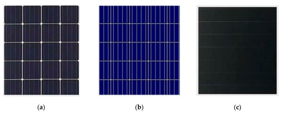
Figure 1.
Photovoltaic (PV) modules: (a) mono-crystalline, (b) multi-crystalline and (c) thin film.
The PV system model’s parameters used in this study is shown in Table 1. The total power output of system was calculated using weather data, including the GHI, DNI, DHI, wind speed and air temperature. The DNI can be estimated from the GHI using the direct insolation solar code (DISC) model described in [53,54]. Technical specifications of the PV modules and PV inverters are presented in Section 5. We applied a performance degradation rate of 0.64%/year according to [55].

Table 1.
PV system parameters.
2.2. Wind Energy Conversion System
The power of the wind turbine is produced through wind blowing the blades to drive a rotor axis. The mechanical energy produced at the rotor axis is used to drive an electrical generator to generate electricity. Small wind turbines can be classified into two types, as shown in Figure 2a (horizontal axis) and Figure 2b (vertical axis type). The power output of the vertical wind turbine can be calculated using Equation (1) [56] and Equation (2) [57] from the manufacturer’s power curve.
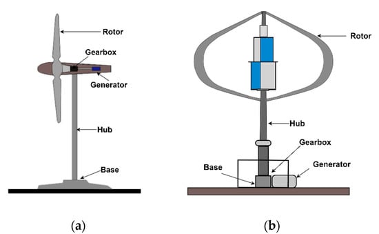
Figure 2.
Small wind turbines: (a) horizontal axis, (b) vertical axis.
is the smoothed power curve value at standard wind speed in the power curve; . is the wind speed; is the interval between and ; and is the standard deviation and can be calculate using Equation (2). The value for can be determined using the measurement accuracy of wind speed. For example, if the wind speed measurement accuracy is 0.1 m/s, can be set to a value of 0.1 m/s.
Wind speed varies according to height, and the structure of the terrain also influences the vertical wind profile. We can calculate wind speed at the hub height of the wind turbine, , using a logarithmic wind profile [58], as shown in Equation (3).
where is the wind speed at hub height, ; is the wind speed from the weather/measurement data; is the height at which measurements are taken; and is the surface roughness length.
Vertical wind turbines used in this study were modeled using windpowerlib/Python [59] and the wind turbines’ power curve from the manufacturer’s data sheet. The performance degradation rate of the vertical wind turbines were not studied extensively; thus, we used a degradation rate of 1.6%/year [60], similar to onshore horizontal wind turbines. The details of the wind turbines and other components are provided in Section 4.
2.3. Battery Bank
Battery banks are often used with PV and wind energy systems, or with a combination of both, to store the excess energy produced by the system. This stored energy can be later used to provide electricity when the generation system cannot meet the energy demand required by the load. The state-of-charge (SoC) of the battery also determines the quantity of electricity for the charge and discharge cycle. The SoC of the battery at time t can be obtained using Equation (4).
where is the input/output power of the battery in watts (negative during discharging and positive during charging mode); is the time step at which the SoC is calculating, in this case 1 h; is the round-trip efficiency defined as 80% for charging and 100% for discharging models; denotes the number of batteries in the battery bank; is the nominal capacity in Ah; is the nominal voltage of the battery; and is the self-discharge rate of the battery (%/hour). The battery bank’s SoC is constrained to a maximum SoC limit, , and a minimum limit, .
2.4. Hybrid Energy System
In this study, we refer to the optimal sizing of a grid connected to a HES system according to economic and environment benefit considerations. Two reference buildings were considered in this work: (a) residential buildings in an urban scenario, referred to as “Residential”; and (b) residential buildings in a rural scenario that is also used for limited farm activities, except storage, and is referred to as “Farm”. The energy required by these two types of building are mostly used for heating, domestic hot water, air-conditioning and other electrical peripherals. The configuration considered in this study is shown in Figure 2 and consists of a wind energy conversion system (WECS), PV system and battery bank. As the both types of buildings are grid-connected, particular attention should be given to the buying and selling strategy of excess power. For this, the HES system should be designed without over-sizing, maximizing the feed-in to the grid and minimizing the overall power bought from the grid.
As shown in Figure 3, the HES system considered in this study consisted of PV modules and a vertical wind turbine with dedicated inverters. A microgrid controller was used to manage the energy produced by these two systems and handle the electricity demand from the load source, i.e., the residential building. Microgrid controller also managed the charging and discharging of the battery bank, including buying and selling the power to the utility grid through a smart meter.
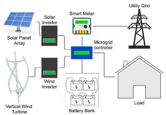
Figure 3.
Schematic diagram of the grid-connected hybrid energy system.
In Figure 4, the process flowchart of the HES simulation is presented. The simulation is initialized at time t = 0, with the hourly weather data and hourly load profile. The PV system’s power output, Ppv, and wind turbine system’s power output, Pwt, were calculated. Residual power, Pres, was calculated by subtracting Ppv and Pwt from the hourly load on the system, PL. If the Pres is greater than zero, the required power is bought from the utility grid, else the battery SoC is checked for maximum SoC. If the SoC is at the maximum level, the residual energy is sold to the grid, else the battery is charged and the SoC is recalculated. If the SoC is greater than or equal to the maximum SoC, the extra power is sold to the utility grid. The simulation then continues the process for maximum time limit, T (175, 200 h, 20 years).
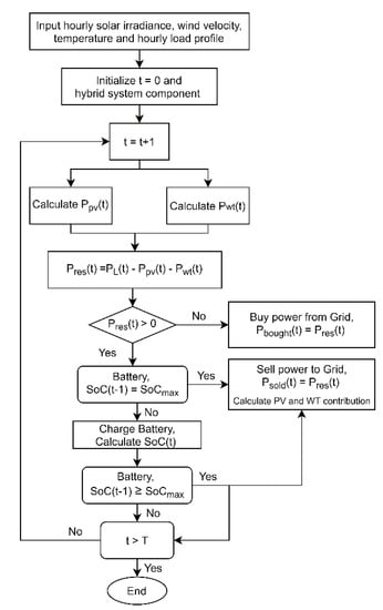
Figure 4.
Process flowchart of the hybrid energy system (HES) simulation.
3. Methodology
3.1. Problem Formulation
Economic objectives of the HES system are often influenced by the government policies of the region. Regional wind and solar attributes also play an important role when choosing the right configuration and sizing for the HES system. Since this study presents a case study of southern Taiwan region, it is important to note the regional cost of electricity bought from the grid and the FiT rates for solar and wind energy. Taiwan Power Company (Taipower) is a state-owned company that provides power to the whole region. The average cost per unit of electricity (kWh) [61] is 0.082 US$. It is important to note that the Taiwan government has specified different FiT rates for electricity generated from rooftop solar panels and onshore wind turbines. The size of the installation is also taken into consideration when evaluating the FiT rates. Therefore, Equation (5), which calculates the cost of the power bought from the grid, must consider these differences in FiT rates. The FiT rate [8] for wind energy from onshore WECS systems smaller than 30 kW capacity is 0.26 US$/kWh and for solar energy from rooftop PV systems with a capacity smaller than 20 kW is 0.19 US$/kWh. With FiT in effect, one of our economic objectives, the net balance of power bought from grid (PB), can be calculated using Equation (5). Another economic objective considered in this study is net present cost (NPC), also referred to as the net present value. The NPC consist of the total capital cost of the HES system (Ccap), replacement cost of batteries in the battery bank (Crep), operating and maintenance cost of the system (Cop) and the total salvage cost of the system (Cs) at the end-of-lifecycle time, T. The method for calculating the NPC is given in Equation (6).
where is the units of power bought from the grid; is the cost of power bought from grid; is the PV power sold to the grid; is the FiT for electricity generated from the PV system; is the WECS power sold to the grid; and is the FiT for electricity generated from wind energy. It should be noted that the microgrid controller shown in the schematic diagram of the HES in Figure 3 is used in all configurations of the HES, therefore its cost is not considered in Ccap; also, the is sensitive to the market prices of fuels used by the electricity provider to generate electricity. After studying the price trends of electricity in Taiwan, an annual increase of 1.86% was applied to the electricity prices. The salvage cost, Cs, of the total system was considered 20% of Ccap for a system lifetime of 20 years.
The environmental objective used in this study was the total contribution to CO2 emissions by the HES. Since the HES configuration used in this study does not include biomass or diesel generators, the contribution to CO2 emissions was calculated by considering the total amount of electricity bought from the grid. According to Taipower’s annual sustainability report [62] for the year 2019, the current CO2 emissions per kWh, CO2e, is 0.421 kg/kWh. Total CO2 emissions, Fe, during the project’s life-time for the grid-connected HES system can be calculated using Pg, as in Equation (7).
Constraints used for our optimization problem are based on the total installation area available Iarea and maximum PV system power PVmax. For this study, the maximum installation area available for urban residential buildings equals 99.17 m2 (30 ping) and for rural residential buildings equals 397 m2 (120 ping). The maximum installation area used in this study corresponds to the average rooftop area available on these types of buildings in Taiwan. Ping is a Chinese unit of measurement for area, 1 ping = 3.3057 m2.
Using the above objectives and constraints, we can formulate our optimization problem for the HES system with a lifecycle period of 20 years, as in Equation (8). The input variables considered for our problem are number of batteries in the battery bank (Nbat), number of wind turbines (Nwt), wind turbine hub height (hhub), wind turbine model (Wtid), number of PV modules in series (Ns) and number of PV modules in parallel (Np); where, the values for each variable are integers, except for hhub.
3.2. Optimization Algorithm
The optimization algorithm deployed in this study is the differential evolution variant of the multi-objective evolutionary algorithm based on decomposition [22,63] (MOEA/D-DE). Multiple studies [64,65] have suggested that the MOEA/D algorithm is more accurate for finding the complex Pareto sets and can handle mixed integer problems better than NSGA-II. The MOEA/D-DE used in this study uses the Tchebycheff decomposition [66] method to decompose objectives into singular objective. This decomposition method converts the multi-objectives into a single distance-based objective by calculating their respective weight. The decomposed objective is the distance from a reference point, an ideal utopia point in criterion space. For constraints violation, we apply penalties to the objectives of the population that violates the defined constraint space. “Kuri’s death penalty” [67] is used for the constrained multi-objective problem defined in the previous section. The objectives were set to a value close to infinity (8.9884 × 10307) according to the rate of satisfied constraints. The Pareto front of the final result was sorted using the method described in [68]. The complete process flowchart of the MOEA/D-DE algorithm used in this study is shown Figure 5a and the flow chart of the HES optimization is shown is Figure 5b. The optimization was carried out using the Pygmo/Python library, which is the python binding of the C++ library Pagmo [69]. The parameters used for the MOEA/D-DE algorithm for a population size of 55 are as follows: (a) generations = 60, (b) neighborhood size = 20, (c) crossover probability = 0.9, (d) differential evolution parameter = 0.5, (e) distribution index = 20 (polynomial mutation), (f) neighborhood consideration probability = 0.8 and (g) diversity preservation by inserting and replacing the old with a new population every generation = 2.
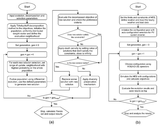
Figure 5.
(a) Process flow chart of the multi-objective evolutionary algorithm based on decomposition (MOEA/D-DE). (b) HES optimization flow chart.
4. Data and Discussion
4.1. Köppen–Geiger Climate Classification System
The Köppen–Geiger scale was first introduced by Wladimir Köppen in 1900 to quantitatively classify the world’s climates. This scale/system was later improved by Rudolf Geiger in 1954 and 1961. Therefore this system of climate classification was named the Köppen–Geiger climate classification system [70]. This scale/system classifies the climates into five primary groups, 14 secondary groups and six tertiary groups, as presented in [71]. These classifications are made using weather data like air temperature, wind speed, average precipitation, solar irradiance, etc.
Climate classification can be used to find a similar climate area for a specific location. In Figure 6, the Köppen–Geiger map of Taiwan is shown. Most of the population in Taiwan resides near the coastal areas and the central areas are mainly mountainous terrain. The northern Taiwan region is mainly composed of a temperature climate zone with no dry season and hot summers (Cfa), as well as temperate climate with dry winters and hot summers (Cwa). The southern region of Taiwan is mainly composed four climate types: (a) Tropical, rainforest (Af); (b) Tropical, monsoon (Am); (c) Tropical, savannah (Aw); and (d) Temperate, dry winters and hot summers (Cwa). The Af climate zone in southern Taiwan mainly comprise the Chenggong and Changbin Township of Taitung County. It also extends into the two outer islands, namely, Green Island and Orchid Island. Located on the east coast of Taiwan, the Af zone typically receives average monthly precipitation [72] of over 70 mm, and the average temperature during winter is above 20 °C and above 30 °C during summer. The Am zone comprises some of the non-coastal areas of the Tainan and Kaohsiung counties. Most of the residential areas in Pingtung County falls under the Am climate zone, including some of the southern coast of the Taitung county. This climate zone in Taiwan typically receives yearly accumulated precipitation of 2500 mm, with the driest month being January. The average high temperature in the Am zone is around 25.6 °C and average low temperature around 14.7 °C. The Aw climate zone comprises the coastal areas of the Tainan and Kaohsiung counties. These are the most populated areas of southern Taiwan. The coastal area of Tainan County receives most of the rain during the months of June, July and August. The average annual maximum temperature is 28.7 °C, with warmest month being July and the coolest month being January—when the average minimum temperature can be below 14 °C. Taitung County also have areas in the Cwa climate zone, which comprises the Luye, Guanshan and Chishang townships. These townships are located in re-entrant terrain and receives an average monthly rainfall of over 300 mm during the months of June, July, August and September. The average maximum temperature in this region can reach up to 30 °C during summer and average minimum temperature drops as low as 15 °C during winter. The precipitation varies 328 mm between the driest (January) and wettest month (July).
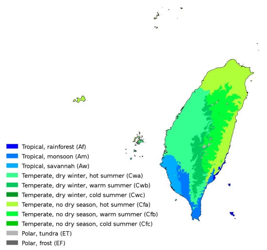
Figure 6.
Köppen–Geiger climate map of Taiwan [71].
Since the climate has an immediate effect on the cooling and heating needs of residential buildings, we use this classification system to model the hourly load demand of the buildings. Hourly load-profile data are not available for the residential buildings in Taiwan; therefore, we chose a climate location similar to the one that is to be modeled, the United States of America’s Köppen–Geiger map (Figure 7), and extracted the data from the Open Energy Information website’s hourly load-profile dataset from the Typical Meteorological Year version 3 (TMY3) database [73]. More information about hourly load data is provided in the next subsection.
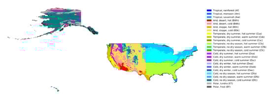
Figure 7.
Köppen–Geiger climate map of the USA [71].
4.2. Locations and Hourly Load Profile
The four locations used in this study, based on the four major climate areas, are shown in Figure 8. We chose the residential building’s load profile from the TMY3 dataset by matching the Köppen–Geiger scale of the location in the dataset to that of the location in our study. The locations chosen from the TMY3 dataset are listed in Table 2. Since this study considers two types of residential buildings, the load profile for the “Farm” building type is adjusted 30% more than “Residential”, while the “Residential” building type’s load profile is kept the same as the base load profile from the TMY3 dataset. The hourly load profiles of the different locations for “Residential” buildings are presented in Figure 9.
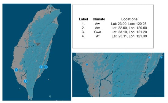
Figure 8.
Locations used for the optimization study, chosen based on the Köppen–Geiger climate scale.
Table 2.
The locations and their corresponding hourly load profiles from the TMY3 dataset.
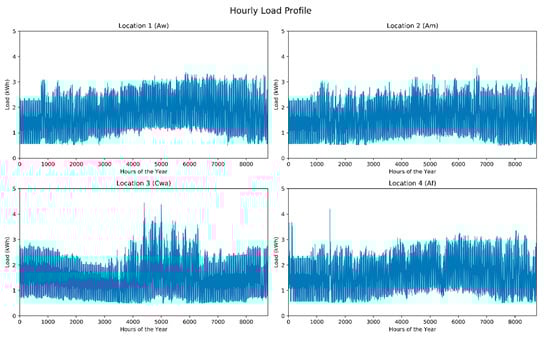
Figure 9.
Hourly load profiles for the different locations.
Location 1, which falls under the Aw climate zone, shows a gradual increase in hourly load from the month of January to December, with the highest average hourly load observed during the period of June to August, which is consistent with the constant usage of air conditioning due to hot and wet weather. The highest variation in hourly load is observed during the winter due to hot water requirements. Location 2 (Am) and Location 4 (Cwa) followed the similar hourly trend as Location 1. At Location 3, we can observe large variations in electricity usage during the period of June to August, due to higher temperatures and high precipitation.
4.3. Weather Data
This study used the European Centre for Medium-Range Weather Forecasts ReAnalysis (ERA5) dataset [74]. The ERA5 dataset contains global reanalysis weather data with several atmospheric, land and sea level weather attributes. For this study, we accessed the hourly GHI, wind speed at 10 m height and air temperature variables for the year 2019 of four locations using the ERA5/Python library [75]. From Figure 10, it can be observed that Location 3 and 4 receives the least GHI throughout the year with the months of December and January being lower than 500 W/m2. Location 1 and 2 receive the highest hourly GHI throughout the year with the average maximum monthly GHI being over 600 W/m2. However, during the months of June, July and August, we can observe several variations in GHI at all locations due to the rainy season. Location 4 has the highest wind speed throughout the year, as shown in Figure 11. Locations 1, 2 and 3 show similar wind speed trends with the average wind speed value being slightly over 3 m/s. The air temperature variation between day and night is also the highest at Locations 1, 2 and 3, as shown in Figure 12. We can also confirm from Figure 12 that summer and winter temperature variations correspond to that of the hourly load profile, shown in Figure 9. It should be noted that Location 3 is a location in re-entrant terrain and, due to a higher humidity and temperature, it leads to higher electricity usages during summer.
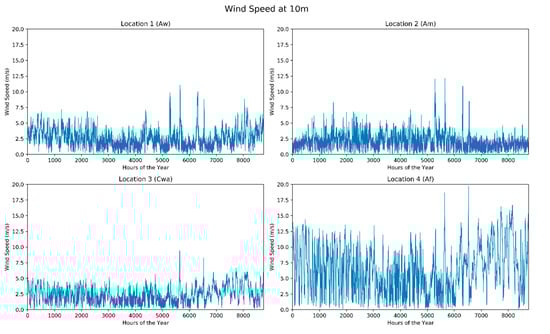
Figure 10.
Hourly solar irradiance data for the four locations.
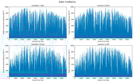
Figure 11.
Hourly wind speed at 10 m height for the four locations.
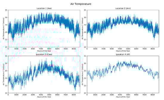
Figure 12.
Hourly air temperature for the four locations.
5. HES Components
5.1. PV Components
The photovoltaic system modeled in this study used multi-crystalline PV modules from Motech Industries with a maximum power output of 330 Watts. The CEC database values for this module’s parameters vary slightly from the data sheet. Therefore, we used the CEC parameters, as shown in Table 3, to keep the model consistent with the Pvlib/Python model. The inverter for the PV system model was chosen from a range of inverters, as shown in Table 4, according to total power output of the modules in the system. The PV system model is programmed to choose the inverter of a suitable power range according to the PV module’s maximum power output (Psys). The efficiency curve for the inverters can be found in the CEC database. The cost data listed in Table 3 and Table 4 are the average of multiple online references.
Table 3.
Single diode model parameters of the Motech Industries IM72D3 solar panel.
Table 4.
Inverters used for the PV system.
5.2. WECS Components
For this study, we used three vertical axis wind turbines to create our configuration pool for optimization. Each wind turbine was assigned an integer identification value, ranging from 0 to 2. Turbines used for this study were from a regional manufacturer named Hi-VAWT Technology Corp. The technical details of the wind turbines are provided in Table 5 and the power curve data of each turbine is shown in Figure 13. Cost data listed in Table 5 are the sum of the vertical axis wind turbine and the wind power controller. The hub height is considered as the sum of the building height (25 m) and the turbine hub height.
Table 5.
Components of the wind energy conversion system (WECS).
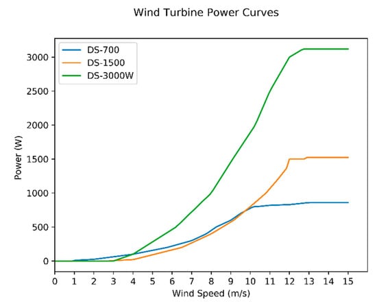
Figure 13.
Power curves of the vertical axis wind turbines.
5.3. Battery
Lead–acid batteries were used in this study to model the battery bank. Replacement of batteries are considered after every fourth year, which is also the end of the average standard warranty time for such batteries. The average self-discharge rate for lead–acid batteries [76] are reported to be 5% per month (720 h). The specifications of the battery used to model the battery bank are listed in Table 6.
Table 6.
Battery specifications.
6. Results
6.1. Optimization Results
The HES sizing optimizations are carried out for all four locations discussed in Section 4.2 for the two building types “Residential” and “Farm”. The Pareto set plots for the three objectives for each location are presented in Figure 14, Figure 15, Figure 16 and Figure 17, respectively.
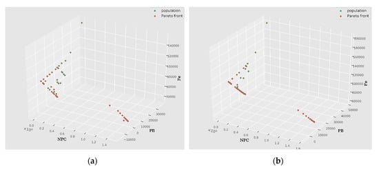
Figure 14.
Pareto optimal sets for Location 1 (Aw), for building type (a) Residential and (b) Farm.
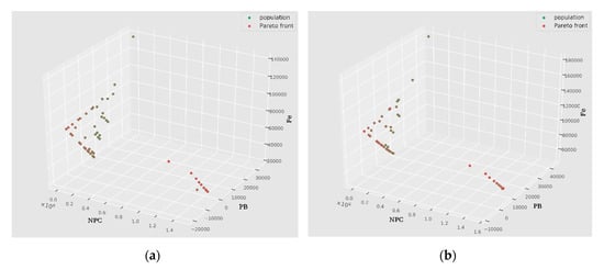
Figure 15.
Pareto optimal sets for Location 2 (Am), for building type (a) Residential and (b) Farm.
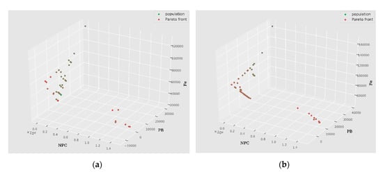
Figure 16.
Pareto optimal sets for Location 3 (Cwa), for building type (a) Residential and (b) Farm.
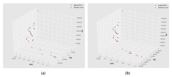
Figure 17.
Pareto optimal sets for Location 4 (Af), for building type (a) Residential and (b) Farm.
In Figure 14a, the Pareto sets shows a gradual decrease between PB and Fe, which is consistent with the fact that a lower amount of power bought from the grid decreases the carbon emission contribution of the building. The value of PB was below zero for the NPC values below 270,000. However, in this range of the same NPC value, multiple possibilities for PB and Fe can be observed. However, in order to reach the Fe target of below 40,000, a significant increase in NPC is required. Due to the larger area constraint in “Farm” buildings (Figure 14b), the multiple possibilities of PB and Fe for same value of NPC is reduced and we can observe a less complicated tradeoff curve. The higher NPC for lower Fe arises due to the higher initial capital cost required by the wind turbines. Since the wind energy is not abundant in Location 1, as shown in Figure 11, the optimization converges towards a higher number of wind turbines.
At Location 2, the GHI (Figure 10) and wind speed (Figure 11) trends are similar to that of Location 1. In addition to the climate properties, the hourly load characteristics are also very similar. Therefore, in Figure 15, we can observe similar Pareto sets for the converged results. We can find some dissimilarity in terms of the tradeoff between NPC with Fe and NPC with PB, for the NPC values below 300,000. At Location 2, the optimization results show a higher number of multi-configuration possibilities for these two pairs of objectives.
Wind energy availability is lowest at Location 3, as can be seen in Figure 11. Although, during the summer, the amount of GHI (Figure 10) is higher but the lower average GHI values during winter certainly affects the Pareto front of the “Residential” buildings. As shown in Figure 16a, the climate characteristics, high usage of electricity during summer (Figure 9) and lower area availability leads to convergence of PB and Fe in a very narrow range of NPC with multiple possibilities. We can observe several configurations of variables that lead to different PB and Fe values for an NPC in the range of 10,000 to 280,000. For “Farm” buildings, due to a higher availability of installation area, the trade-off curves are less complicated, as shown in Figure 16b.
At Location 4, an abundance of wind energy leads to multiple possibilities for wind turbine configurations. The DS-700 wind turbine is a cheaper option when it comes to the initial capital cost and this is evident from the trade-off curve shown in Figure 17a,b. For both types of buildings, we can see the several options that provide lower PB and Fe values in the NPC range of 400,000 to 1,000,000. To better visualize the interaction between the three objectives and six variables, the pairwise plots of the optimization results are shown in Figure 18 and Figure 19.
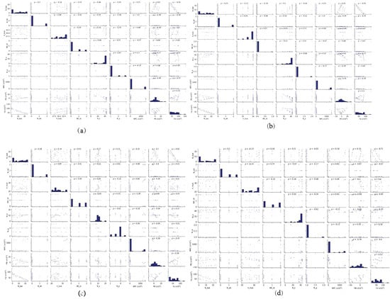
Figure 18.
Pairwise plots of the optimized solution for “Residential” buildings for (a) Location 1 (Aw), (b) Location 2 (Am), (c) Location 3 (Cwa) and (d) Location 4 (Af).
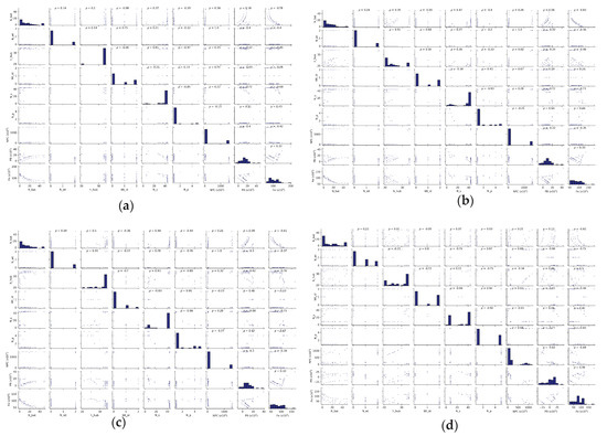
Figure 19.
Pairwise plots of the optimized solution for “Farm” buildings for (a) Location 1 (Aw), (b) Location 2 (Am), (c) Location 3 (Cwa) and (d) Location 4 (Af).
Pairwise plots provides a better representation of the trade-off between different objectives and their relationships with the variables. From Figure 18 and Figure 19, we can clearly see that for the same value of NPC, there are multiples possibilities for the PB and Fe sets for each location, which confirms the complexity of the HES optimization problem at these four locations. The number of batteries, Nbat, in the battery bank has a high influence on the NPC; therefore, we can see multiple options. Similarly, as the value of Nbat increases, the total carbon emission of the building also decreases. The higher number of batteries leads to a higher PB, since the excess power generated by the HES system is used to charge the batteries instead of being sold to the utility grid. Therefore, the higher feed-in rates are not well utilized to maximize the savings from the HES system. Therefore, the trade-off curve suggests having a lower number of batteries is preferable for profit-maximization. For Locations 1, 2 and 3, the wind speed values are not high; therefore, in the optimized results we only see two options: either 0 turbines or 2 turbines. However, for Location 4, we can find diverse combinations for WCES. Since the initial capital cost for the PV modules are much lower than the wind turbines, all the optimization results tend to converge towards a total number of 44 PV modules. The distribution of Ns and Np varies at different location but does not show any significant interaction with the other variables and objectives. For both types of buildings, the wind turbine hub height does not show any significant effect for Location 1 and 2. However, for Location 3 and 4, multiple options for hub height can be observed in the converged population. We classified the results of the Pareto set into four strategies: minimum NPC (other than no HES), minimum PB, minimum Fe and balanced. The method of finding the balanced configuration is discussed in the subsection below.
6.2. Optimal Configuration Selection
The goal of multi-objective optimization is to find the optimal configuration considering several objectives simultaneously. The Pareto front obtained from the process can be overwhelmingly difficult to interpret. A balanced HES system should maximize the savings (for electricity cost) while meeting the environmental goals set by government policies. Therefore, in this study we considered a method for calculating the fitness of each objective by using the “No HES” system as a reference. Using Equation (11), we can assign a fitness value to the individual sets in the Pareto front. The fitness value is calculated by subtracting the sum of the NPC and PB of the configuration under consideration from the PB of the “No HES” configuration, and then dividing the PB of the “No HES” to obtain the ratio of improvement. We constrain the results by setting the fitness values to negative infinity, for a Pareto set that has Fe values greater or equal to 50% of the Fe of the “No HES” configuration. Therefore, the higher the fitness value of the Pareto value indicates higher savings with respect to the “No HES” configuration, while satisfying the government target of a 50% reduction in GHS/CO2 reduction. A balanced strategy can be deployed for choosing the best configuration, which has the highest fitness value. We also consider the minimum value configuration for each objective for comparison. In Table 7 and Table 8 we list the “No HES”, minimum NPC, minimum PB, minimum Fe and balanced (highest fitness) for each location and two types of buildings.
Table 7.
Optimization results for the “Residential” buildings at the four locations.
Table 8.
Optimization results for the “Farm” buildings at the four locations.
Using a balanced strategy of finding fitness index (Equation (11)), one can not only obtain higher returns on initial investment (NPC) but also meet the environmental goals. As shown in Table 7, For the “Residential” building type, a balanced strategy can save 46%, 49%, 17% and 35% for the cost of the electricity against buildings without the HES at the four locations, respectively. For the “Farm” building type, our balanced strategy can obtain savings of 21%, 32%, 24% and 9% at the four locations, respectively, for total project lifecycle time. It is important to note that the least NPC strategy has the highest investment-to-saving ratio; however, it does not meet the environmental goals set by local government. The least PB strategy mainly focuses on selling more electricity generated from the HES system back to the utility grid. Therefore, optimization results include two wind turbine configurations with no battery bank for all locations. Lower PB strategy systems incorporate more wind turbines due to higher FiT rates for wind energy. As shown in Figure 18 and Figure 19, a larger battery bank capacity can reduce the dependence on the grid and reduce the total carbon emission contribution of the buildings. From Table 7 and Table 8, it is evident in least the Fe strategy that by incorporating the maximum battery bank capacity, a WCES system and PV system, the HES systems at all locations can reduce total carbon emissions substantially at the cost of a very high NPC.
As reducing the environmental impact is one of the important goals of any HES system, a balanced strategy can be utilized for minimizing the CO2 emissions, while preserving the economic interest of independent electricity users. Using a balanced strategy, for “Residential” buildings (Table 9), the average NPC for all four locations is approximately US$25,000, with Location 4 requiring the least NPC. The HES installation for “Residential” buildings at Location 1 can generate the maximum savings over the lifecycle period of 20 years and has a shorter payback period of 10.7 years. Location 2 also generates high savings and has the shortest payback period of 10.3 years. It is due to the highest availability of solar energy throughout the year at Locations 1 and 2, as discussed in Section 4. However, at Location 3, the highest reduction in CO2 emissions can be observed but at a price of a higher NPC, less savings and a longer payback period. A longer payback period for Location 3 can be justified due to less availability of solar energy and higher electricity demands. As shown in Table 9, the average NPC for “Farm” buildings at the four locations is approximately US$26,250. The savings are also much lower than that of “Residential” buildings, with Location 3 being the only exception. On average, payback period for “Farm” buildings are longer than residential buildings. When using models with higher number of parameters and more precise equations, the simulation results tends to be more realistic but at the cost of computation time. The grid-connected HES model used in this study takes an average of 4.7 s/evaluation (using multi-threading and multi-processing techniques). The optimization problem considers 25 × 3 × 150 × 3 × 44 × 6 combinations (8,910,000) for “Residential” and 17,820,000 combinations for “Farm” building types. Using the enumerative technique, it would take 1.33 years and 2.66 years for two types of buildings. However, using the MOEA/D_DE technique it only requires 55 × 60 combinations (3300) for each building type, approximately equal to 4.3 h.
Table 9.
Economic and environmental analysis of a balanced selection strategy for a lifetime cycle of 20 years.
Optimization and simulation evaluations were conducted in the Python programming language on a notebook PC with an Intel i5 7th generation CPU with 2 physical cores (with hyper-threading) and 8 GB RAM.
7. Conclusions
In this paper, we have presented a case study for multi-objective sizing optimization of a grid-connected HES system for the southern Taiwan region. For the first time, a case study is presented for the Taiwan region considering the Köppen–Geiger climate scale. The climate classification scale was used to find a similar hourly load for each climate zone and building type under consideration. We also present an optimization framework and HES simulation model by taking Taiwan’s electricity cost trends, feed-in tariff rates and government policies into account. Objectives considered for the multi-objective HES optimization are derived from the environment and economic demands of the region. The area constraint was derived from the average rooftop area available for the building type and the PV system constraints were derived from the feed-in tariff rates for electricity generated from solar power. The problem studied in this research targets the geographical area of southern Taiwan and its socio-political situation in contrast to the HES system feasibility for residential users. The contribution of this study can be summarized as follows:
- This study provides a general multi-objective optimization framework for an HES sizing, considering the climate classification of location, feed-in tariff, installation area restrictions and maximum HES capacity restrictions using economic and environmental objectives. A case study of four locations in the southern Taiwan region is presented, for two types of residential buildings, which analyzes the HES system feasibility and optimal sizing using multi-objective Pareto set analysis.
- A balanced strategy for choosing the optimal configuration of an HES system is introduced that maximizes the savings for independent users while meeting the government set goals of reducing carbon emissions.
From the analysis of the Pareto front results of the HES optimization at different locations and building types, this case study has shown the following in context of the objectives stated:
- Feed-in tariff can significantly affect the economic objectives. However, the higher NPC of wind turbines makes it economically unfeasible for residential users to utilize the maximum potential of wind energy, even in presence of significantly higher FiT rates for wind-generated electricity.
- Higher NPC systems, which includes wind turbines, does not significantly reduce the reliability on the utility grid, neither affect the total cost of power bought from the grid during the project lifetime, as PV-only systems with a lower NPC can provide a significant reduction in PB.
- An HES configuration with two small wind turbines and a high battery bank capacity can significantly reduce the total carbon emission contribution of a residential building and reduce the cost of power bought from the grid.
- A balanced strategy for choosing an HES configuration that can generate maximum profit for independent electricity users while preserving the environment can be utilized to encourage the usage of an HES among residential buildings.
A balanced strategy for choosing an HES configuration proposed in this study can be used as reference by the residential users. The case study of the four locations presented in this paper has revealed the following characteristics of a balanced HES installation at the four locations:
- For the two building types at all four locations studied in this research, an HES with a 15 kW PV system and a small capacity battery bank can generate maximum savings for the user and also reduces the carbon emission contribution by more than 50%.
- Solar energy availability of a location does not significantly affect the NPC. However, it does significantly affect the amount of power bought and sold to the grid. The total payback period of the system is also increased at Locations 3 and 4, where less GHI throughout the year is observed. However, at Locations 1 and 2, where solar energy availability is higher, a payback period shorter than 11 years is observed for “Residential” and 15.7 and 13.6 years is observed for “Farm” buildings, respectively.
In order to reach the environmental goal of reducing CO2 emissions, a battery bank is crucial to the HES. As shown in this study, a battery bank of capacity ranging from 700 Ah to 1100 Ah is suitable for “Residential” and 900 Ah to 1900 Ah is suitable for “Farm” buildings. The future directions for this work include creating an hourly electric load database for the different cities and locations of Taiwan using TMY3 data and average monthly electricity consumption for the location based on different building types. A graphical user interface also will be developed for the sizing optimization framework presented in this study. Improvements in simulation and evaluation time is another possibility. We will also explore other meta-heuristic algorithms, in order to improve the convergence time.
Author Contributions
Conceptualization, K.S.; data curation, K.S.; formal analysis, J.-C.T.; investigation, S.-C.W.; methodology, K.S. and J.-C.T.; software, K.S.; supervision, J.-C.T. and S.-C.W.; visualization, K.S.; writing—original draft, K.S.; writing—review and editing, J.-C.T. and S.-C.W. All authors have read and agreed to the published version of the manuscript.
Funding
This research received no external funding.
Acknowledgments
The authors acknowledge the constructive comments provided by reviewers during the review process that helped improving the reporting method and quality of this paper.
Conflicts of Interest
The authors declare no conflict of interest.
Abbreviations
| Cbat | Nominal capacity of individual battery |
| Ccap | Total capital cost of the HES system |
| CEC | California Energy Commission |
| Cg | Cost of electricity bought from the utility grid |
| CO2e | CO2 emission |
| Cop | Operating and maintenance cost of the HES system |
| Crep | Replacement cost for batteries |
| Cs | Salvage cost of the HES system at the end-of-lifecycle time |
| DHI | Direct horizontal irradiance |
| DISC | Direct insolation solar code |
| DNI | Direct normal irradiance |
| F | Objective function |
| Fe | Total CO2 emission |
| FiT | Feed-in-tariff |
| FiTpv | Feed-in tariff for PV energy |
| FiTwe | Feed-in tariff for wind energy |
| gen | Generation |
| GHG | Greenhouse gas |
| GHI | Global horizontal irradiance |
| HES | Hybrid energy system |
| hhub | Wind turbine hub height |
| hmeasured | Wind speed data measurement height |
| HRES | Hybrid renewable energy system |
| Iarea | Installation area constrain for HES system |
| IL | Light generated current (PV module) |
| Imp | Maximum power current (PV module) |
| Isc | Short circuit current (PV module) |
| lat | Latitude |
| lon | Longitude |
| MOEA/D | Multi-objective evolutionary algorithm based on decomposition |
| MOEA/D-DE | Differential evolution variant of multi-objective evolutionary algorithm based on decomposition |
| Nbat | Number of batteries in battery bank |
| Ncell | Number of cells (PV module) |
| No-HES | Without hybrid energy system |
| Np | Number of PV modules in parallel |
| NPC | Net present cost |
| Ns | Number of PV modules in series |
| NSGA-II | Non-dominated sorting genetic algorithm |
| Nwt | Number of wind turbines |
| PB | Total cost of power bought from grid |
| Pg, Pbought | Power bought from utility grid |
| PL | Power required by electrical load |
| Ppv | Power produced by PV system |
| Prated | Rated Power |
| Pres | Residual power |
| Psmooth | Smoothed power curve at standard wind speed in manufacturer power curve |
| Psold | Power sold to utility grid |
| Pspv | PV power sold to utility grid |
| PSTC | Power at standard test condition (PV module) |
| Pswe | Wind energy power sold to utility grid |
| Psys | Total PV system power |
| Pt | Power at time step t |
| PV | Photovoltaic |
| PVmax | Maximum PV power constrain |
| Pwt | Power produced by wind turbines |
| Rsh | Shunt resistance (PV module) |
| SoC | State of charge of battery |
| t | Time step |
| T | Maximum time step, end-of-life cycle time |
| TNOCT | Nominal operating condition temperature (PV module) |
| Vbat | Nominal voltage of individual battery |
| vhub | Wind speed at wind turbine hub height |
| vi | Wind speed at interval I in the manufacturer’s power curve |
| Vmp | Maximum power voltage (PV module) |
| Vrated | Rated output voltage |
| vstd | Standard wind speed in the manufacturer’s power curve |
| WECS | Wind energy conversion system |
| WT | Wind turbine |
| Wtid | Wind turbine identification number |
| z0 | Surface roughness length |
| Δt | Interval between two time steps |
| Δvi | Wind speed step in manufacturer power curve |
| ηbat | Round-trip efficiency of an individual battery |
| ηsd | Self-discharge rate of an individual battery |
References
- World Meteorological Organization. WMO Statement on the Status of the Global Climate in 2019; World Meteorological Organization: Geneva, Switzerland, 2019; ISBN 9789263111081. [Google Scholar]
- Rogelj, J.; Shindell, D.; Jiang, K.; Fifita, S.; Forster, P.; Ginzburg, V.; Handa, C.; Kheshgi, H.; Kobayashi, S.; Kriegler, E.; et al. Mitigation Pathways Compatible with 1.5 °C in the Context of Sustainable Development; Intergovernmental Panel on Climate Change: Genève, Switzerland, 2018; p. 82. [Google Scholar]
- Global Climate Action Summit. Report of the Secretary-General on the 2019 Climate Action Summit and the Way Forward in 2020; Global Climate Action Summit: San Francisco, CA, USA, 2019. [Google Scholar]
- IRENA. Future of Solar Photovoltaic: Deployment, Investment, Technology, Grid Integration and Socio-Economic Aspects; IRENA: Abu Dhabi, UAE, 2019; ISBN 9789292601560. [Google Scholar]
- IRENA Future of Wind Deployment. Investment, Technology, Grid Integration and Socio-Economic Aspects; IRENA: Abu Dhabi, UAE, 2019; ISBN 9789292601553. [Google Scholar]
- Wu, T. Green Energy Promotion Policies and Industry Development in Taiwan; Industrial Technology Research Institute: Zhudong, Taiwan, 2015. [Google Scholar]
- Bureau of Energy Ministry of Economic Affairs. Policy for Promoting Renewable Energy in Taiwan; Bureau of Energy Ministry of Economic Affairs: Taipei, Taiwan, 2013. [Google Scholar]
- Bureau of Energy Ministry of Economic Affairs. 2020 Feed-In Tariffs of Renewable Energy; Bureau of Energy Ministry of Economic Affairs: Taipei, Taiwan, 2020; pp. 1–2. [Google Scholar]
- Environmental Protection Administration. Taiwan’s Strategies and Achievements in Greenhouse Gas Emission Reduction. Environ. Policy Mon. 2015, 18, 1–12. [Google Scholar]
- International Carbon Action Partnership, Berlin. Taiwan passes GHG Reduction Law and Considers Emissions Trading, 22 June 2015. Available online: https://icapcarbonaction.com/en/news-archive/285-taiwan-passes-ghg-reduction-law-and-considers-emissions-trading (accessed on 3 January 2020).
- Conti, P.; Lutzemberger, G.; Schito, E.; Poli, D.; Testi, D. Multi-objective optimization of off-grid hybrid renewable energy systems in buildings with prior design-variable screening. Energies 2019, 12, 3026. [Google Scholar] [CrossRef]
- Singh, R.; Bansal, R.C.; Singh, A.R.; Naidoo, R. Multi-objective optimization of hybrid renewable energy system using reformed electric system cascade analysis for islanding and grid connected modes of operation. IEEE Access 2018. [Google Scholar] [CrossRef]
- González, A.; Riba, J.R.; Rius, A.; Puig, R. Optimal sizing of a hybrid grid-connected photovoltaic and wind power system. Appl. Energy 2015, 154, 752–762. [Google Scholar]
- González, A.; Riba, J.R.; Rius, A. Optimal sizing of a hybrid grid-connected photovoltaic-wind-biomass power system. Sustainability 2015, 7, 12787–12806. [Google Scholar]
- Taebnia, M.; Heikkilä, M.; Mäkinen, J.; Kiukkonen-Kivioja, J.; Pakanen, J.; Kurnitski, J. A qualitative control approach to reduce energy costs of hybrid energy systems: Utilizing energy price and weather data. Energies 2020, 13, 1401. [Google Scholar] [CrossRef]
- Alaaeddin, M.H.; Zakaria, A.; Jani, J.M.; Seyajah, N. Optimization techniques and multi-objective analysis in hybrid solar- wind power systems for grid-connected supply. IOP Conf. Ser. Mater. Sci. Eng. 2019, 538, 6–12. [Google Scholar] [CrossRef]
- Eriksson, E.L.V.; Gray, E.M. Optimization of renewable hybrid energy systems—A multi-objective approach. Renew. Energy 2018, 133, 971–999. [Google Scholar] [CrossRef]
- Mohammed, O.H.; Amirat, Y.; Benbouzid, M. Economical evaluation and optimal energy management of a stand-alone hybrid energy system handling in genetic algorithm strategies. Electronics 2018, 7, 233. [Google Scholar] [CrossRef]
- Murty, V.V.S.N.; Kumar, A. Multi-objective energy management in microgrids with hybrid energy sources and battery energy storage systems. Prot. Control. Mod. Power Syst. 2020, 5, 1–20. [Google Scholar] [CrossRef]
- Mazzeo, D.; Oliveti, G.; Baglivo, C.; Congedo, P.M. Energy reliability-constrained method for the multi-objective optimization of a photovoltaic-wind hybrid system with battery storage. Energy 2018, 156, 688–708. [Google Scholar] [CrossRef]
- Deb, K.; Pratap, A.; Agarwal, S.; Meyarivan, T. A fast and elitist multiobjective genetic algorithm: NSGA-II. IEEE Trans. Evol. Comput. 2002, 6, 182–197. [Google Scholar] [CrossRef]
- Zhang, Q.; Li, H. MOEA/D: A multiobjective evolutionary algorithm based on decomposition. IEEE Trans. Evol. Comput. 2007, 11, 712–731. [Google Scholar] [CrossRef]
- Mohamad, F.; Teh, J.; Abunima, H. Multi-objective optimization of solar/wind penetration in power generation systems. IEEE Access 2019, 7, 169094–169106. [Google Scholar] [CrossRef]
- Ren, H.; Lu, Y.; Wu, Q.; Yang, X.; Zhou, A. Multi-objective optimization of a hybrid distributed energy system using NSGA-II algorithm. Front. Energy 2018, 12, 518–528. [Google Scholar] [CrossRef]
- Li, F.F.; Qiu, J.; Wei, J.H. Multiobjective optimization for hydro-photovoltaic hybrid power system considering both energy generation and energy consumption. Energy Sci. Eng. 2018, 6, 362–370. [Google Scholar] [CrossRef]
- Yong, Y.; Rong, L. Techno-economic optimization of an off-grid solar/wind/battery hybrid system with a novel multi-objective differential evolution algorithm. Energies 2020, 13, 1585. [Google Scholar] [CrossRef]
- Xiao, J.; Li, J.J.; Hong, X.X.; Huang, M.M.; Hu, X.M.; Tang, Y.; Huang, C.Q. An improved MOEA/D based on reference distance for software project portfolio optimization. Complexity 2018, 2018, 1–16. [Google Scholar] [CrossRef]
- Ju, Y.; Zhang, S.; Ding, N.; Zeng, X.; Zhang, X. Complex network clustering by a multi-objective evolutionary algorithm based on decomposition and membrane structure. Sci. Rep. 2016, 6, 33870. [Google Scholar] [CrossRef]
- Ellefsen, K.O.; Lepikson, H.A.; Albiez, J.C. Multiobjective coverage path planning: Enabling automated inspection of complex, real-world structures. Appl. Soft Comput. J. 2017, 61, 264–282. [Google Scholar] [CrossRef]
- Hsiao, J.C.; Shivam, K.; Chou, C.L.; Kam, T.Y. A shape design optimization of a robot arm using a surrogate-based evolutionary approach. Appl. Sci. 2020, 10, 2223. [Google Scholar] [CrossRef]
- Ming, M.; Wang, R.; Zha, Y.; Zhang, T. Multi-objective optimization of hybrid renewable energy system using an enhanced multi-objective evolutionary algorithm. Energies 2017, 10, 674. [Google Scholar] [CrossRef]
- Control, J.; Muthukumar, R.; Balamurugan, P. A novel power optimized hybrid renewable energy system using neural computing and bee algorithm. Automatika 2019, 60, 332–339. [Google Scholar]
- Aziz, A.S.; Tajuddin, M.F.N.; Adzman, M.R.; Ramli, M.A.M.; Mekhilef, S. Energy management and optimization of a PV/diesel/battery hybrid energy system using a combined dispatch strategy. Sustainability 2019, 11, 683. [Google Scholar] [CrossRef]
- Mohamed, A.A.A.; Ali, S.; Alkhalaf, S.; Senjyu, T.; Hemeida, A.M. Optimal allocation of hybrid renewable energy system by multi-objectivewater cycle algorithm. Sustainability 2019, 11, 6550. [Google Scholar] [CrossRef]
- Shi, B.; Wu, W.; Yan, L. Size optimization of stand-alone PV/wind/diesel hybrid power generation systems. J. Taiwan Inst. Chem. Eng. 2017, 73, 93–101. [Google Scholar] [CrossRef]
- Maheri, A. Multi-objective design optimisation of standalone hybrid wind-PV-diesel systems under uncertainties. Renew. Energy 2014, 66, 650–661. [Google Scholar] [CrossRef]
- Donado, K.; Navarro, L.; Quintero, M.C.G.; Pardo, M. HYRES: A multi-objective optimization tool for proper configuration of renewable hybrid energy systems. Energies 2019, 13, 26. [Google Scholar] [CrossRef]
- Fu, T.; Wang, C. A novel ensemble wind speed forecasting model in the longdong area of loess plateau in china. Math. Probl. Eng. 2018, 2018, 672–685. [Google Scholar] [CrossRef]
- Ascencio-Vásquez, J.; Brecl, K.; Topič, M. Methodology of Köppen-Geiger-Photovoltaic climate classification and implications to worldwide mapping of PV system performance. Sol. Energy 2019, 191, 672–685. [Google Scholar] [CrossRef]
- De Carli, M.; Bernardi, A.; Cultrera, M.; Santa, G.D.; Di Bella, A.; Emmi, G.; Galgaro, A.; Graci, S.; Mendrinos, D.; Mezzasalma, G.; et al. A database for climatic conditions around europe for promoting GSHP solutions. Geosciences 2018, 8, 1–19. [Google Scholar] [CrossRef]
- Mazzeo, D.; Baglivo, C.; Matera, N.; Congedo, P.M.; Oliveti, G. A novel energy-economic-environmental multi-criteria decision-making in the optimization of a hybrid renewable system. Sustain. Cities Soc. 2020, 52, 101780. [Google Scholar] [CrossRef]
- Braun, R.; Haag, M.; Stave, J.; Abdelnour, N.; Eicker, U. System design and feasibility of trigeneration systems with hybrid photovoltaic-thermal (PVT) collectors for zero energy office buildings in different climates. Sol. Energy 2020, 196, 39–48. [Google Scholar] [CrossRef]
- Hossain, M.; Mekhilef, S.; Olatomiwa, L. Performance evaluation of a stand-alone PV-wind-diesel-battery hybrid system feasible for a large resort center in South China Sea, Malaysia. Sustain. Cities Soc. 2017, 28, 358–366. [Google Scholar] [CrossRef]
- Holmgren, W.; Hansen, C.; Mikofski, M. pvlib python: A python package for modeling solar energy systems. J. Open Source Softw. 2018, 3, 884. [Google Scholar] [CrossRef]
- De Soto, W.; Klein, S.A.; Beckman, W.A. Improvement and validation of a model for photovoltaic array performance. Sol. Energy 2006, 80, 78–88. [Google Scholar] [CrossRef]
- Kratochvil, J.A.; Boyson, W.E.; King, D.L. Photovoltaic Array Performance Model. Ph.D. Thesis, Sandia National Laboratories, Albuquerque, NM, USA, December 2004. [Google Scholar]
- Reda, I.; Andreas, A. Solar position algorithm for solar radiation applications. Sol. Energy 2004, 76, 577–589. [Google Scholar] [CrossRef]
- Ineichen, P.; Perez, R. A new airmass independent formulation for the Linke turbidity coefficient. Sol. Energy 2002, 73, 151–157. [Google Scholar] [CrossRef]
- Perez, R.; Ineichen, P.; Moore, K.; Kmiecik, M.; Chain, C.; George, R.; Vignola, F. A new operational model for satellite-derived irradiances: Description and validation. Sol. Energy 2002, 73, 307–317. [Google Scholar] [CrossRef]
- Hay, J.E.; Davies, J.A. Calculation of the solar radiation incident on an inclined surface. Proc. First Can. Sol. Radiat. Data Work. 1980, 23, 301–307. [Google Scholar]
- System Advisor Model. Available online: https://github.com/NREL/SAM/tree/develop/deploy/libraries (accessed on 10 February 2020).
- King, D.; Gonzalez, S.; Galbraith, G.; Boyson, W. Performance model for grid-connected photovoltaic inverters. Sandia Natl. Lab. 2007, 38. [Google Scholar] [CrossRef]
- Maxwell, E.L. A Quasi-Physical Model for Converting Hourly Global Horizontal to Direct Normal Insolation; Solar Energy Research Inst.: Golden, CO, USA, 1987; pp. 35–46. [Google Scholar]
- Maxwell, E. DISC Model. Available online: https://www.nrel.gov/grid/solar-resource/disc.html (accessed on 12 February 2020).
- Jordan, D.C.; Kurtz, S.R. Photovoltaic degradation rates—An analytical review. Prog. Photovolt. Research Appl. 2012. [Google Scholar] [CrossRef]
- Knorr, K. Modellierung Von Raum-Zeitlichen Eigenschaften Der Windenergieeinspeisung Für Wetterdatenbasierte Windleistungssimulationen; Kassel University Press GmbH: Kassel, Germany, 2016. [Google Scholar]
- Staffell, I.; Pfenninger, S. Using bias-corrected reanalysis to simulate current and future wind power output. Energy 2016, 114, 1224–1239. [Google Scholar] [CrossRef]
- Gasch, R.; Twele, J. Wind Power Plants; Springer: Berlin, Germany, 2012; ISBN 978-3-642-22937-4. [Google Scholar]
- Sabine, H.; Schachler, B.; Krien, U. Windpowerlib—A python library to model wind power plants (Version V0.2.0). Zenodo 2019. [Google Scholar] [CrossRef]
- Staffell, I.; Green, R. How does wind farm performance decline with age? Renew. Energy 2014, 66, 775–786. [Google Scholar] [CrossRef]
- Taiwan Power Company. Rate Schedules. Available online: https://www.taipower.com.tw/upload/317/2018032816540459885.pdf (accessed on 24 January 2020).
- Taiwan Power Company. 2019 Sustainability Report. Available online: https://csr.taipower.com.tw/upload/132/2019110109130980581.pdf (accessed on 24 February 2020).
- Liu, B.; Fernández, F.V.; Zhang, Q.; Pak, M.; Sipahi, S.; Gielen, G. An enhanced MOEA/D-DE and its application to multiobjective analog cell sizing. In Proceedings of the 2010 IEEE Congress on Evolutionary Computation, Barcelona, Spain, 18–23 July 2010. [Google Scholar]
- Li, H.; Zhang, Q. Multiobjective optimization problems with complicated pareto sets, MOEA/ D and NSGA-II. IEEE Trans. Evol. Comput. 2009, 13, 284–302. [Google Scholar] [CrossRef]
- Peng, W.; Zhang, Q.; Li, H. Comparison between MOEA/D and NSGA-II on the multi-objective travelling salesman problem. Stud. Comput. Intell. 2009, 171, 309–324. [Google Scholar]
- Ma, X.; Zhang, Q.; Tian, G.; Yang, J.; Zhu, Z. On tchebycheff decomposition approaches for multiobjective evolutionary optimization. IEEE Trans. Evol. Comput. 2018, 22, 226–244. [Google Scholar] [CrossRef]
- Kuri Morales, A.F.; Quezada, C.C. A universal eclectic genetic algorithm for constrained optimization. In Proceedings of the 6th European Congress on Intelligent Techniques & Soft Computing EUFIT’98, Aachen, Germany, 7–10 September 1998. [Google Scholar]
- Deb, K.; Agrawal, S.; Pratap, A.; Meyarivan, T. A fast elitist non-dominated sorting genetic algorithm for multi-objective optimization: NSGA-II. CEUR Workshop Proc. 2000, 1133, 849–858. [Google Scholar]
- Biscani, F.; Izzo, D.; Jakob, W.; GiacomoAcciarini, M.; Märtens, M.C.; Mereta, A.; Kaldemeyer, C.; Lyskov, S.; Corlay, S. esa/pagmo2: Pagmo 2.15.0. Zenodo 2020. [Google Scholar] [CrossRef]
- Wilcock, A.A. Köppen after fifty years. Ann. Assoc. Am. Geogr. 1968, 58, 12–28. [Google Scholar] [CrossRef]
- Beck, H.E.; Zimmermann, N.E.; McVicar, T.R.; Vergopolan, N.; Berg, A.; Wood, E.F. Present and future köppen-geiger climate classification maps at 1-km resolution. Sci. Data 2018, 5, 1–12. [Google Scholar] [CrossRef] [PubMed]
- Central Weather Bureau, Taiwan. Available online: https://www.cwb.gov.tw/eng/ (accessed on 22 April 2020).
- Office of Energy Efficiency & Renewable Energy (EERE)Commercial and Residential Hourly Load Profiles for all TMY3 Locations in the United States. Available online: https://openei.org/doe-opendata/dataset/commercial-and-residential-hourly-load-profiles-for-all-tmy3-locations-in-the-united-states (accessed on 14 March 2020).
- Copernicus Climate Change Service (C3S) (2017): ERA5: Fifth Generation of ECMWF Atmospheric Reanalyses of the Global Climate. Copernicus Climate Change Service Climate Data Store (CDS). Available online: https://cds.climate.copernicus.eu/cdsapp#!/home (accessed on 20 March 2020).
- Petrelli, P. coecms/era5: Python base codes to interface the CDS api and automate ERA5 download: First release v0.1. Zenodo 2019. [Google Scholar] [CrossRef]
- Garche, J.; Dyer, C.K.; Moseley, P.T.; Ogumi, Z.; Rand, D.A.J.; Scrosati, B. Encyclopedia of Electrochemical Power Sources, 2nd ed.; Elsevier Science: Amsterdam, The Netherlands, 2009; ISBN 9780444520937. [Google Scholar]
© 2020 by the authors. Licensee MDPI, Basel, Switzerland. This article is an open access article distributed under the terms and conditions of the Creative Commons Attribution (CC BY) license (http://creativecommons.org/licenses/by/4.0/).