Identification of the Building Envelope Performance of a Residential Building: A Case Study

Abstract

Since households are one of the most energy-intensive sectors in Europe, retrofit of dwellings is promoted to increase energy efficiency. Recent research, however, shows that the energy performance after retrofit does not always meet the target values, which can be caused by amongst other things, a deviating building envelope performance. This paper compares the theoretical and measured building envelope performance for a real-life case study in post-retrofit state, in order to illustrate the limitations of calculation methods and characterization models. First, the performance is evaluated on building scale by verifying the correspondence between the default theoretical heat loss coefficient (HLC) and the measured HLC, which was determined by following the guidelines formulated within IEA EBC Annex 58 and Annex 71. In order to illustrate the limitations of the standard calculation method in real-life conditions, the theoretical variability of the HLC is evaluated, generated by variating infiltration heat losses and heat exchange with neighboring dwellings. Second, the performance is investigated on a component scale by assessing the theoretical and measured thermal resistances, identified from heat flux tests. Additionally, nonhomogeneous assembled components and air leaks are simulated to verify probable causes for the locally varying measured values and to illustrate the limitations of calculations and characterization methods. The results illustrate the limitations of the calculation methods by the assessment of the strong variability of the theoretical HLC, depending on assumptions regarding infiltration and heat exchange with neighboring dwellings. In addition, component simulations indicated that deficiencies on a component scale could be caused by a nonhomogeneous assembly and air cavity flows of the component. Moreover, a detailed assessment of an unreliable thermal resistance illustrates the limitations of the used characterization method. Finally, a contrast was found between the quite good performance on building scale (15% deviation between the theoretical and measured HLC) and poor performance on a component scale (only one out of nine monitored components met their theoretical target values), which illustrates the complexity of the building envelope performance.

1. Introduction

In order to adhere to the European climate targets [1] set to reduce greenhouse gas emissions and increase energy efficiency and the share of renewables, the total energy use needs to be decreased. Since households in Europe are responsible for circa 25% of the total energy use in Europe [2], mandatory criteria prescribing a minimum insulation quality, energy efficiency, and a minimum share of renewable energy [3,4] were imposed on the energy performance of buildings. These criteria should not only be obligatory for newly built dwellings, but also for existing dwellings, as 66.4% of European dwellings were originally constructed before 1980 [5].

The actual energy performance of newly built or retrofitted dwellings, however, can strongly deviate from the theoretical design value. This effect, commonly known as the energy performance gap, is identified in literature for several case studies. For instance, in Belgium, 20 case studies were assessed for which the actual energy use was significantly lower than the theoretical energy use [6]. The energy performance gap was also assessed in Germany for 60 renovated apartments, which showed the impact of user behavior, the malfunctioning of the heating system, and a mismatch between the observed and expected domestic hot water use [7]. In addition to these case studies, a Dutch large scale study of all energy-labeled dwellings [8] showed that the energy performance gap depends on the energy quality of the dwellings: for energy-efficient dwellings, the actual energy use is underestimated by theoretical calculations, while for energy-intensive dwellings, the actual energy use is overestimated.

The different causes of the energy performance gap mentioned in literature can be classified into three main categories [9]: errors in the design stage, in the construction stage, and in the operational stage. First, in the design stage, incorrect modeling tools or methods may lead to unreliable predictions. For instance, monthly quasi-steady-state modeling tools are often used to estimate the energy use or energy savings of a renovated dwelling. Due to the use of standardized boundary conditions concerning default outdoor temperatures and heating schedules, these tools calculate a normalized energy use rather than realistic energy use. Furthermore, building services might not perform as specified by the manufacturer and erroneous design of the building services might lead to several imperfections such as low boiler efficiency, inefficient ventilation heat recovery [7,10], a poor (usage of the) heating control system [7,11,12] or a low Coefficient of Performance (COP) of the heat pump [7,12,13]. Second, deficits during the construction stage can also contribute to the energy performance gap. Several monitoring campaigns pinpointed building envelope imperfections such as thermal bridges, air leaks, or other defects [11,13,14]. Third, in the operational stage, standardized boundary conditions considering simplified user behavior have an important contribution to the difference between the measured and the predicted energy performance. To this end, previous research identified amongst others a constant indoor temperature and simplified ventilation losses as key assumptions that significantly influence the energy performance gap [15,16,17,18]. Additionally, model specifications such as the number of incorporated zones were also shown to have a big impact [15].

In order to assess the share of building envelope imperfections in the energy performance gap, measurements can be carried out on two scales to identify the building envelope performance: on full building scale or on building component scale. On the building scale the overall building envelope performance can be assessed theoretically by determining the heat loss coefficient (HLC) following general building physical principles of transmission and infiltration [19]. In addition, the HLC can also be measured by performing a quasi-steady state test such as the co-heating test, a short, time-dynamic method such as the quick U-building method [20], a dynamic test in which the heating power is controlled by (pseudo-) random signals, or onboard monitoring [21]. Several methods to identify the HLC were further elaborated by Bauwens [22]. On a component scale, the transmission heat losses can be evaluated by estimating the thermal resistances for each building component. These thermal resistances can either be calculated theoretically following the standards [23] or be measured by the heat flux meter method [24]. Since different models can be applied to estimate the thermal resistance from measurements, Deconinck [25] formulated some recommendations on the most reliable estimation models.

The theoretical value of the HLC is also used in the European standard NBN EN 12831:2003 [26] which presents a methodology to calculate the design heat load of a building. In this generic, some boundary conditions are standardized: a constant infiltration rate is assumed and heat losses towards neighboring dwellings, through the party walls, are neglected. Several researchers, however, showed the importance of taking into account variable infiltration rates [27,28] and heat losses through party walls [29,30,31]. Hence, a standardized HLC might be a rather limited representation of the building envelope performance of a real-life case study, which is why on-site measurements are applied more and more, as seen in [11,13,32,33].

In this context, this paper aims to illustrate the limitations of the methods to identify the envelope performance by comparing the theoretical building envelope, as defined in standards and building designs, with the measured building envelope, as identified from in situ measurements. To this end, the difference between the theoretical and measured building envelope performance will be assessed for a case study for which an energy performance gap was identified. The post-retrofit building envelope of the case study is assessed on building scale and on a component scale. On building scale, the performance will be evaluated by comparing the theoretical HLC-values to the HLC identified by in situ measurements following the guidelines of IEA EBC Annex 58 [34]. In addition, the limitations of the standard calculation methods for the real-life case study are shown, as the theoretical HLC is subject to various assumptions regarding the boundary conditions, such as infiltration rates and heat exchange through the party walls. On a component scale, the performance will be assessed by comparing the theoretical and measured thermal resistance for some of the building components. To explain the discrepancies in thermal resistances, some hypotheses are raised and verified by means of simulations of local inhomogeneities. Additionally, the limitations of the steady-state methods, applied to calculate the thermal resistance, are illustrated by simulating the impact of dynamical boundary conditions and by evaluating the robustness of the identification model.

This paper consists of five remaining sections. First, the case study specifications are further presented. Subsequently, the methods to identify the HLC on building scale are discussed, followed by the methods to distinguish the performance of the building components and the monitoring campaign of the case study. Next, the results for the full building envelope and for the building components are summarized. Finally, discussion and conclusions are presented.

2. Description of the Case Study

The case study was part of the “Mutatie +” pilot project, of which the aim was to develop a retrofit strategy with prefabricated units, combining energy efficiency, lifelong living, and an economic retrofit. The project was supported by Flanders Innovation and Entrepreneurship (VLAIO). More information and videos on the retrofit measures can be found on the website of the “Platform for Renovation” [35]. The dwelling was originally built as a terraced miners’ dwelling in the 1930s and was renovated in 2016 towards the nearly zero energy building standard. In order to achieve a theoretical decrease in total energy use of 90%, the building envelope was insulated, the energy system was renewed, and renewable energy units were added. In Figure 1 the floor plans and the section of the retrofitted dwelling are visualized, including six thermal bridges (blue 1 to 6—see Section 3.1.2 and Section 4.1.1) and three simulated building components (orange A to C—see Section 3.2.2 and Section 4.2.3). The building geometry has been changed during retrofit: the back extension of the dwelling was demolished and replaced by a more compact, insulated, prefabricated unit. The changes are indicated in black at the dwellings’ section, while the original building components are indicated in gray. In order to define the building envelope performance, the dwelling was being monitored both in the occupied and unoccupied state.

The retrofit was designed to improve the insulation quality of the building envelope: The infiltration rate was aimed to decrease to 0.2 air changes per hour, while the average target value of the thermal transmittance (U-value) decreased from 1.12 W/(m²K) to 0.32 W/(m²K). An overview of the U-values, together with the surface areas per envelope component can be found in

Table 1. Target U-values (W/(m²K)) and surface areas (m²) of the pre-retrofit and post-retrofit building envelope.

Building Component	Pre-Retrofit	U-Value W/(m2K)	Area m2	Post-Retrofit	U-Value W/(m2K)	Area m2
Windows and glass doors	Double glazing PVC frame	2.30	17.4	Triple glazing PVC frame	1.00	17.1
Roof window	-	-	-	Double glazing PVC frame	1.6	1.7
Front facade	Uninsulated cavity wall	1.13	19.7	Uninsulated cavity wall + 12 cm PUR	0.23	19.7
Rear facade	Uninsulated cavity wall	1.13	16.3	Prefabricated insulated component	0.12	11.4
Rear facade extension	Uninsulated cavity wall	1.45	29.8	Prefabricated insulated component	0.24	4.8
Pitched roof	Wooden frame + 8 cm mineral wool	0.68	54.6	Wooden frame with 25 cm mineral wool	0.17	50.4
Flat roof extension	Wooden frame without insulation	1.98	30.5	Prefabricated insulated component	0.21	21.5
Floor on the ground (Main building)	Uninsulated concrete slab	0.57	18.9	Uninsulated concrete slab	0.57	18.9
Floor on the ground (Extension)	Uninsulated concrete slab	0.57	28.2	Prefabricated insulated component	0.19	22.3
Floor above cellar	Uninsulated concrete slab	0.75	17.8	Concrete slab + 8 cm PUR	0.28	17.8

. These U-values are calculated according to the national standard (NBN B 62-002:2008 [36]) and the international standard for heat transfer through the ground (EN ISO 13370:2004 [37]).

Table 1 shows that the pre-retrofit dwelling was uninsulated, except for the pitched roof and the double-glazing windows. Subsequently, in the post-retrofit state, the dwelling is fully insulated, except for the floor on the ground of the original dwelling, which takes approximately one third of the full floor surface area (see gray floor on the ground on the building section in Figure 1. Two types of retrofit measures were carried out on the exterior walls: the front facade was insulated by adding an exterior layer of insulation, while the rear facades were completely replaced by prefabricated insulated components.

Besides fully insulating the building envelope, the building energy systems were renewed. For the space heating of the building, the boiler (with a theoretical full load generation efficiency of 92.7%) and radiators have been removed and replaced by a condensing boiler (with a theoretical full load generation efficiency of 96.2%) with air heating system together with a mechanical ventilation system with heat recovery. Next, renewable energy units were added to the building: a solar boiler for domestic hot water generation and photovoltaic cells for electricity generation.

Despite the complete retrofit, the realized energy savings, derived from pre-retrofit and post-retrofit monitoring of the energy use, were found to be significantly lower than the theoretical energy savings of 90%, as shown in

Table 2. Theoretical and measured primary energy use in kWh per year, and the resulting energy savings in percentage.

Type of Energy Use	Pre-Retrofit Energy Use (kWh)	Post-Retrofit Energy Use (kWh)	Energy Savings (%)
Theoretical	155,151.5	14,885.9	90%
Measured year 1	21,030.8	11,411.7	46%
Measured year 2	21,030.8	18,533.6	12%
Measured year 3	21,030.8	13,327.3	37%

. The theoretical energy use shown in this table was calculated by means of the Belgian calculation procedure, a monthly quasi-steady-state method [38], while the energy use was measured for one year in pre-retrofit and for three consecutive years in post-retrofit state. This measured energy use is corrected for the outdoor climate by means of the heating degree day method [39].

The total yearly energy use for the three post-retrofit years varied significantly, which is caused by different inhabitants successively living in the dwelling. This induces a large variation in energy savings, although they are all significantly lower than the theoretical 90%. Furthermore, Table 2 also shows a significant difference between theoretical and measured values both in pre- and post-retrofit state. In pre-retrofit state, the measured energy use is 86% lower than the theoretical value, while in post-retrofit state the measured values are subsequently 23% lower, 25% higher, and 10% lower. Several causes for the differences between theoretical and measured values were previously mentioned, such as heating behavior of the occupants, the rebound and prebound effect, and underperformance of the building energy system or building envelope imperfections. One of these causes, the building envelope performance of the renovated case, will be assessed in the following sections in order to verify whether this could have a share in the difference between the post-retrofit theoretical and measured energy use.

3. Research Methodology

This section explains the methodology of the building envelope assessment of the case study. First, the performance on building scale will be defined by means of the theoretical and measured HLC. In addition, the impact of assumptions regarding boundary conditions will be defined in a sensitivity analysis of the theoretical HLC. Secondly, to identify the performance on a component scale, the methods to identify the thermal resistances from in situ measurements will be explained, as well as the simulations of three of the components. Lastly, the measurement campaigns performed in the case study are summarized.

3.1. Building Scale

The HLC is composed of the transmission heat losses H_tr and the infiltration heat losses H_inf and will be calculated following general building physical principles [19] which were also applied in former research [21,22,31,40,41,42,43] and in the European standard NBN EN 12831 [26]. Next, the measured HLC will be identified from the co-heating test and compared to the theoretical HLC. Finally, the impact of the assumptions regarding the boundary conditions will be assessed for the theoretical HLC by (1) implementing different ways to estimate the infiltration rate, (2) simulating the effect of thermal bridges and (3) assessing the impact of the indoor temperature on the heat exchange through the party walls.

3.1.1. Theoretical Heat Loss Coefficient

The theoretical heat loss coefficient (HLC_T) can be calculated from Equations (1)–(5).

$$HL{C}_T=H_{tr}+H_{inf}$$

(1)

$$H_{tr}=H_{tr,e}+H_{tr,g}+H_{tr,u}$$

(2)

$$H_{tr,x}=\left({\displaystyle \sum }_j\left(U_{j,x}{A}_{j,x}\right)+{\displaystyle \sum }_k\left(l_{k,x}{\psi }_{k,x}\right)\right)\ast b_{tr,x}$$

(3)

$$b_{tr,u}=\frac{T_i-T_u}{T_i-T_e}\mathrm{or}{b}_{tr,u}=\frac{H_{ue}}{H_{iu}+H_{ue}}$$

(4)

$$H_{inf}=c_a{\rho }_a{n}_a{V}_i$$

(5)

The theoretical HLC is composed of the transmission heat losses H_tr and the infiltration heat losses H_inf (Equation (1)). First, the transmission heat losses H_tr are calculated as a summation of three heat flows: H_tr,e towards the exterior, H_tr,g towards the ground and H_tr,u towards unconditioned spaces (Equation (2)). Each of these transmission heat flows x is composed of the heat losses through linear thermal bridges ${\psi }_{k,x}$ and the heat losses through the building components, of which the U-values (W/(m²K)) and the surface areas A (m²) are multiplied (Equation (3)). In order to account for various temperature differences over the building components a correction factor b_tr,x is applied. This factor is equal to 1 for the heat losses towards the exterior, calculated from the floor geometry for the heat losses towards the ground and defined as a ratio for unconditioned rooms. The latter ratio can be calculated in two ways (Equation (4)): either as the ratio of temperature differences (temperature of the interior zone T_i, of the unconditioned zone T_u and of the exterior T_e) or as the ratio of heat losses (heat loss from the unconditioned zone to the exterior H_ue and from the interior zone to the unconditioned zone H_iu).

Second, the infiltration heat losses H_inf are calculated from the specific heat capacity of air c_a (J/(kg·K)), air density ρ_a (kg/m³), infiltration rate per hour n_a (1/h), and the net air volume V_i (Equation (5)). The infiltration rate can be calculated theoretically as a function of the surface area of the building envelope using default infiltration rates. In the European standard default, infiltration rates are imposed as a function of the quality of the window seals [26], while in the regional Flemish standard, the default infiltration rate is a constant value (12 m³/(h·m²) at a 50 Pa indoor-outdoor pressure difference) [38]. To avoid interference of the quality of window seals, the latter value is used here as default for the infiltration rate.

3.1.2. Measured Heat Loss Coefficient

Besides the HLC_T, the measured value (HLC_M) will be estimated from a co-heating test [14]. In this test a dwelling is heated at a constant indoor temperature for more than two weeks, while several parameters are monitored: the heating power ${\mathsf{\varphi }}_h$, the heat losses towards the neighboring zones ${\mathsf{\varphi }}_{tr,n}$, the indoor temperatures of all rooms T_i, the outdoor temperature T_e, and the global horizontal solar radiation I_sol. Following the recommendations of Bauwens and IEA EBC Annex 58 [22,34], HLC_M is estimated most correctly from the co-heating test if dynamic behavior is incorporated in the model. Therefore, an Auto-Regressive model with eXogenous inputs (ARX-model, see Equation (6)) is used. In this model, dynamic behavior is incorporated by means of backshift operators (polynomials $\mathsf{\Phi }\left(B\right)$, ω_i(B), ω_e(B), and ω_sol(B)) applied on the inputs and outputs, which yields that values of previous time steps are also considered [34].

$$\begin{gathered} \mathsf{\Phi }\left(B\right)\left[{\mathsf{\varphi }}_h-{\mathsf{\varphi }}_{tr,n}\right]={\omega }_i\left(B\right)T_{i,avg,j}+{\omega }_e\left(B\right)T_{e,j}+{\omega }_{sol}\left(B\right)I_{sol}+{ϵ}_j \\ \mathrm{With}HL{C}_M=\frac{{\omega }_i\left(1\right)}{\mathsf{\Phi }\left(1\right)} \end{gathered}$$

(6)

To assess the impact of heat exchange with the neighboring dwellings on the measured HLC, the ARX-model will be applied two times: once with and once without subtracting the heat flow towards the neighboring dwelling ${\mathsf{\varphi }}_{tr,n}$ from the heating power ${\mathsf{\varphi }}_h$ (Equation (6)). If ${\mathsf{\varphi }}_{tr,n}$ is subtracted from ${\mathsf{\varphi }}_h$, the identified HLC_M only incorporates the transmission heat loss towards the exterior, the ground and unconditioned rooms and the infiltration heat losses (in correspondence with Equations (1) and (2)). If the full heating power ${\mathsf{\varphi }}_h$ is incorporated in the model, the identified HLC_M also incorporates the heat exchange with the neighboring dwellings (which can be both a heat loss and a heat gain, depending on the interior temperatures).

3.1.3. Sensitivity of the Theoretical HLC

Besides identifying the building envelope performance, the second aim of this paper is to illustrate the limitations of the calculation methods used to identify the theoretical envelope performance. To fulfill this aim for the HLC, the sensitivity of the theoretical HLC will be tested with respect to the infiltration rate, thermal bridges, and the heat exchange through party walls.

The infiltration rate per hour (Equation (7), n_a in 1/h), used to estimate the infiltration heat losses (Equation (5)), will be estimated in three ways. First, the default infiltration rate is used, as previously described in Section 3.1.1. Second, the infiltration rate will be estimated by applying the rule of thumb [44] on the pressurization test results. This rule states that the infiltration rate is 0.05 times the infiltration rate at a 50 Pa pressure difference (n₅₀ in 1/h). Third, the infiltration rate will be estimated by means of the Lawrence Berkeley National Laboratory (LBNL) model which uses the pressurization test results, indoor temperatures, and weather data. The LBNL-model states that the total infiltration flow rate Q_tot depends on the wind-induced infiltration Q_w [m³/s] and the infiltration due to the stack effect Q_s [m³/s] [45] (Equation (8)).

$$n_a=\frac{Q_{tot}\ast 3600}{V_i}$$

(7)

$$\begin{gathered} Q_{tot}=\sqrt{Q_w^2+Q_s^2} \\ \mathrm{with}{Q}_w=f_w^{*}{A}_0{v}^{\prime }\&Q_s=f_s^{*}{A}_0\sqrt{\Delta T} \end{gathered}$$

(8)

In Equation (8) Q_tot [m³/s] is the total infiltration flow rate, V_i [m³] is the internal volume, $f_w^{*}$ the wind parameter, $f_s^{*}$ the stack parameter, v’ the wind speed measured at the nearby weather station [m/s], ΔT the inside-outside temperature difference [K] and A₀ the total effective leakage area [m²] calculated from the pressurization test for a reference pressure difference of 4 Pa.

It must be emphasized that the values obtained by the first two methods are constant values, while the infiltration rate calculated with the LBNL-method varies in time with the measured wind speed and temperatures. Therefore, the infiltration rate resulting from the LBNL-method will be expressed in the results section by a mean value and standard deviation.

Additionally, thermal bridges are evaluated following the European standard and national guidelines [46,47]. The six thermal bridges of the post-retrofit building envelope, indicated in Figure 1, are simulated with TRISCO, a simulation software from Physibel, in which thermal bridges and heat transfer in 2D and 3D orthogonal building components can be simulated by iteratively solving steady-state energy balances [48].

Thirdly, the transmission heat losses H_tr,in from the interior of the dwelling (i) towards the neighboring heated dwellings (n) will be estimated. While the European standard already incorporates these heat losses (NBN EN 12831:2003 [26]), the regional Flemish calculation procedure does not [38]. Former research, however, illustrated the importance of incorporating the heat losses towards the neighboring zones in the HLC [31]. Hence, the heat exchange H_tr,in is calculated following NBN EN 12831:2003 [26], using Equation (9). Here the heat flows for each party wall k, facing the neighboring heated zone, are corrected with a factor calculated as the ratio of the temperature differences between the indoor temperature in the dwelling (T_i), the neighboring zone (T_n), and the exterior (T_e). Note that this calculation procedure is similar to the estimation of the heat losses towards the unconditioned zones (see correction factor Equation (4)).

$$H_{tr,in}={{\displaystyle \sum }}_k{A}_k\ast U_k\ast \frac{T_i-T_n}{T_i-T_e}$$

(9)

For the calculation of this heat flow, the following assumptions are made: the theoretical U-value of the party walls is assumed to be 1.56 W/(m²K), which corresponds to a full brick wall with a thickness of 20 cm including an interior surface resistance of 0.13 m²K/W on both sides of the wall (following NBN EN ISO 6946:2007 [23]). Moreover, the temperatures in Equation (9) are assumed to be constant because otherwise, H_tr,in would be a time-dependent parameter. Hence, for the interior and exterior temperatures T_i and T_e the average value of the monitoring period is used. The neighboring air temperatures T_n, however, were not measured for the post-retrofit dwelling. Therefore, they are induced from pre-retrofit monitoring results of the surface temperatures at the neighboring side of the party walls. To do so, it is assumed that the measured heat flow from the interior surface to the neighboring surface of the party wall is equal to the heat flow from the interior surface to the air in the neighboring room. The occupants’ heating behavior of the neighboring dwellings is hereby assumed to be similar during the pre-retrofit and post-retrofit states, as the neighbors are elderly people with a constant heating pattern. Additionally, the neighboring dwellings are split into a day-zone and a night-zone, as significant temperature differences were identified. Hence, the heat exchange with four neighboring zones is assessed: the day- and night-zone of the left neighboring dwelling and the day- and night-zone of the right neighboring dwelling.

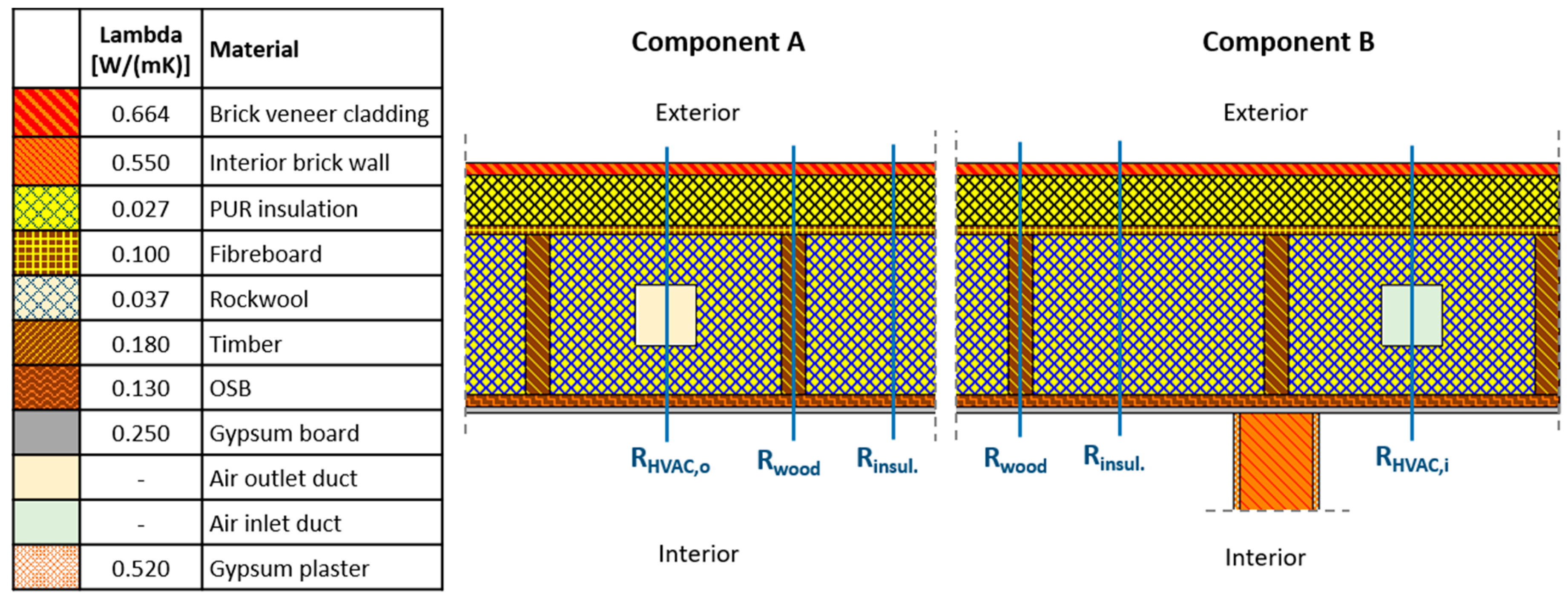
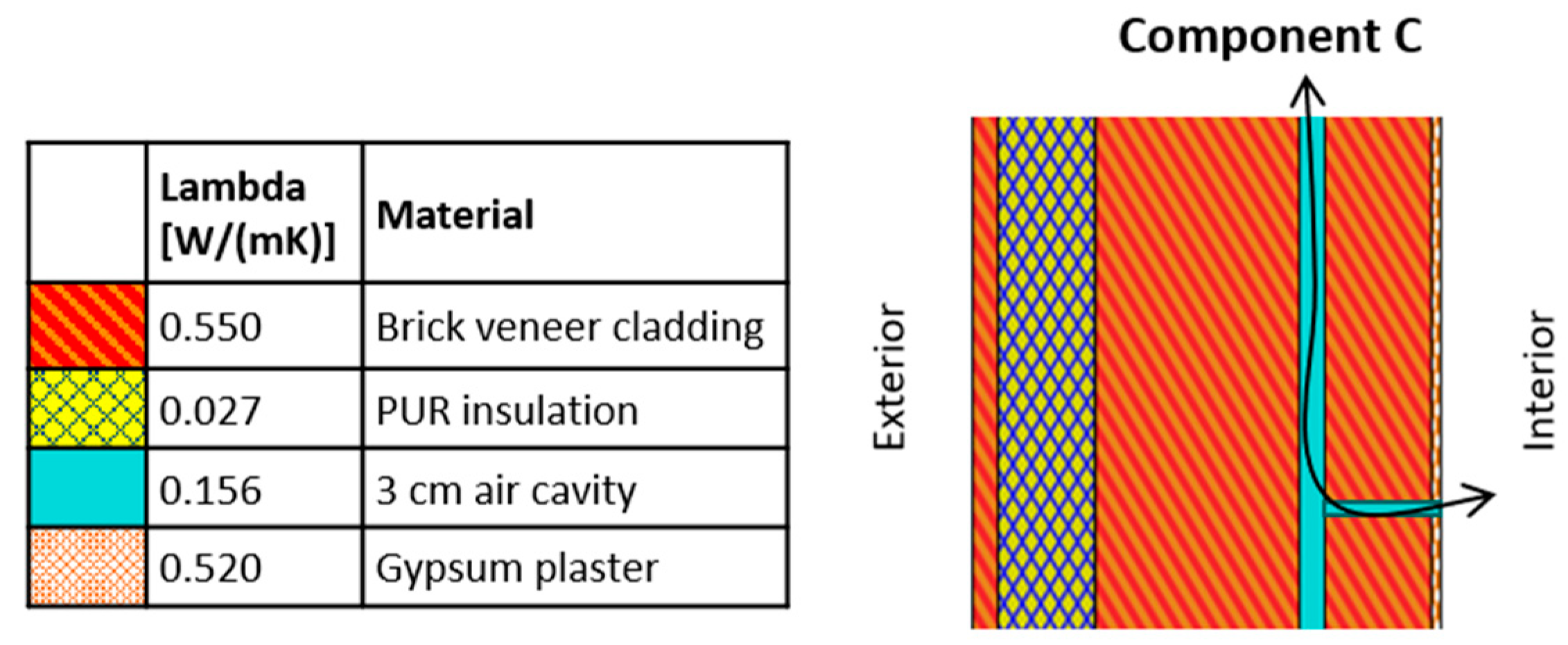
3.2. Component Scale

On a component scale the performance is assessed by means of the thermal resistance, which is identified for specific building components: the front facade, the rear facade, and the floor to the cellar (further discussed in Section 3.3). Similar to the procedure on building scale, first the theoretical and measured values are identified and second they are compared. Additionally, by means of simulations, we will further investigate hypotheses on the most remarkable differences of three measurement locations on the front and rear facade (components A, B, and C in Figure 1). These simulations will also illustrate the limitations of the calculation and characterization methods, used to calculate the theoretical thermal resistance.

3.2.1. Theoretical Thermal Resistance

The theoretical thermal resistances of the tested building components are calculated with the steady-state method defined in the European standard NBN EN ISO 6946:2007 [23]. To incorporate the variability of the material conductivities, the thermal resistance will be defined as an interval, since for the pre-retrofit materials the exact conductivities are unknown and for the new post-retrofit materials the conductivities may differ from the values that were tested in steady-state conditions in laboratories. Therefore, the material conductivities of the old bricks are varied between 0.70 W/(mK) and 1.49 W/(mK), which corresponds to the thermal conductivity for bricks weighing between 1000 and 2000 kg/m³ in outdoor conditions according to the Flemish regional standard [49]. For the new materials, the thermal conductivities provided by the manufacturers are varied with 5%. Furthermore, an equivalent thermal conductivity is calculated for the brick walls as a volume-weighted average between the thermal conductivity of the joints (cement mortar 1.5 W/(mK)) and the bricks.

3.2.2. Measured Thermal Resistance

The measured thermal resistance will be derived from heat flux tests, performed following the European standard (EN ISO 9869-1:2014 [24]). To do so, the dynamic Anderlind’s regression method, shown in Equation (10), is used [50] as recommended in previous research [25]. Note that this is a dynamic method, while the theoretical thermal resistance is calculated by means of steady-state balances.

$$q_j=\frac{1}{R_M}\left(T_{si,j}-T_{se,j}\right)+{\displaystyle \sum }_{l=j-p}^{j-1}{A}_l\left(T_{si,l+1}-T_{si,l}\right)+{\displaystyle \sum }_{l=j-p}^{j-1}{B}_l\left(T_{se,l+1}-T_{se,l}\right)$$

(10)

with

• q = heat flux (W/m²)
• R_M = thermal resistance (m²K/W)
• T_si, T_se = interior (i) and exterior (e) surface temperatures (°C)
• A_l, B_l = regression parameters
• p = number of historical data points that is incorporated
•  = influence time

The thermal resistance R_M, deduced from Equation (10), represents the thermal resistance of the building component without internal and external surface resistances R_si and R_se. In this work, we will assume a constant R_si- and R_se-value following NBN EN ISO 6946:2007 [23]. Therefore, the theoretical reference value of the thermal resistance of the measured building components will be calculated from the target U-values in Table 1 according to the following Equation (11):

$$R_T=\raisebox{1ex}{$1$}\!\left/ \!\raisebox{-1ex}{$U$}\right.-R_{si}-R_{se}\left({\mathrm{m}}^2\mathrm{K}/\mathrm{W}\right)$$

(11)

In order to identify the limitations of Anderlind’s regression method, the robustness of the model, which reflects its capability to identify one single value for the thermal resistance, is defined as a range. To define this range, the thermal resistance is identified for different subsets of the dataset, which are generated by shifting a window of 10 days per hour across the data. The range is then calculated as the difference between the resulting minimum and maximum thermal resistances for all these subsets of the data.

3.2.3. Building Component and Airflow Simulations

Besides the assessment of the thermal resistance, three additional component simulations are performed for two reasons: to verify hypotheses on the causes of the differences between the theoretical and the simulated thermal resistances and to illustrate the limitations of the calculation methods. The exact simulated locations are indicated in Figure 1 (orange components A, B, and C).

Firstly, two horizontal sections A and B of the post-retrofit, prefabricated rear facade will be simulated with TRISCO [48], the software that was also used to calculate the thermal bridges for the sensitivity analysis of the HLC (Section 3.1.3). Figure 2 illustrates the simulated components A and B, chosen because the heat flux tests were performed here (see Section 3.3. Thereby, the exterior and interior are implemented as simplified surface boundary conditions with a constant global surface heat transfer coefficient of 25 W/(m²K) and 8 W/(m²K) and a constant temperature of 0 °C and 20 °C for the exterior and interior respectively. Moreover, the materials are implemented with a fixed thermal conductivity (lambda W/(mK)), as indicated in the legend of Figure 2. In component A, the built-in ventilation duct is an exhaust duct, while in component B it is a supply duct. These ventilation ducts are modeled as a simplified boundary condition with a convective heat transfer coefficient of 3 W/(m²K) and no radiative transfer coefficient, following the international standard ISO 10077-2 implemented in the TRISCO-software [51,52]. The air temperature of the simplified boundary condition is set equal to the indoor temperature (20 °C) for the exhaust duct, while the air temperature in the supply duct is set at 32 °C, which was measured on-site. Note that the air inlet duct is at a quite high temperature because it is part of the heating system. As an output, the simulation will show the temperature distribution and isoflux-lines, which will be assessed to identify the impact of inhomogeneities in a building component, since wooden studs are alternated with insulation and built-in ventilation ducts.

The overall theoretical thermal resistance of non-homogeneous components is theoretically calculated using a volume weighted-average according to the European standard (NBN EN ISO 6946:2007 [23]). Hence, the thermal resistance of the wooden studs and insulation is averaged according to the volume of wood and insulation present in the component. This volume-weighted average thermal resistance, however, can differ significantly from the local thermal resistances. For components A and B, three optional local thermal resistances are indicated: the point where the component is fully insulated (R_insul.), the point where the wooden structure is situated (R_wood) or the point where a ventilation duct is built into the component (R_HVAC).

In addition to components A and B, component C will be simulated, which is a vertical section of the post-retrofit, insulated front facade with an air cavity. The presence of this air cavity was confirmed by on-site destructive research. The exact position of the component is indicated in orange as component C in Figure 1 and the vertical section is illustrated in Figure 3. This figure shows a section of the insulated front facade with at the left the exterior insulation layer, finished with a thin layer of brick veneer cladding, and at the right the original cavity wall consisting of two brick slabs. The impact of air flows in the cavity of this front facade component will be assessed by simulations, since previous research [53,54] showed that the thermal resistance of a building component can significantly be affected by this airflow.

The simulation will be performed with Delphin, a simulation program for the coupled heat, moisture, and matter transport in porous building materials [55]. This software was chosen since Delphin has more advanced dynamic capabilities, e.g., to control air cavity flows and to handle time-dependent boundary conditions [55,56]. In the simulation, the hourly averaged measured interior and exterior temperatures are used as a time-dependent input for component C. The impact of the air cavity ventilation will then be induced by varying the pressure difference between the top and the bottom (as shown in Figure 3). This varying pressure difference yields a variation of the simulated infiltration rate (ACH) of the cavity, of which the values were chosen in accordance with former research [57,58] (−160, −80, −40, −20, 0, 20, 40, 80 and 160 1/h). The output of the simulation is the heat flux, which will be compared to the measured values.

For component C two types of air leaks are assumed, based on the infrared scan of the building shown in Figure 4: (1) air leaks around the window frames, connecting the outside and the air cavity, and (2) air leaks in the inner cavity leaf caused by the openings to support the wooden floor beams, hereby connecting the air cavity and the inside of the dwelling. The air can then either infiltrate in the cavity from the outside or from the inside, depending on the pressure on the facade.

In addition to the simulation of the heat flux through component C, the main driving force for air infiltration, which is the pressure difference generated by an external pressure (P_total), will be evaluated. The correlation between these external pressures and the measured heat fluxes of component C will then be evaluated. The external pressure P_total is composed of two phenomena, similar to the LBNL model: wind pressure (P_w) and stack pressure (P_s). The following Equations (12)–(14) show how these pressures are calculated [59].

$$P_{total}=P_w+P_s$$

(12)

$$P_w=\frac{{\rho }_a{C}_p{v}^2}{2}\left(Pa\right)$$

(13)

$$P_s=-{\rho }_{a}g273\left(h_2-h_1\right)\left[\frac{1}{T_e}-\frac{1}{T_i}\right]\left(Pa\right)$$

(14)

with

• P_w = wind pressure (Pa)
• P_s = stack pressure (Pa)
• ρ_a = air density (kg/m³)
• C_p = wind pressure coefficient
• v = local wind velocity at specified reference height (m/s)
• g = gravitational constant (9.81 m/s²)
• T_e/T_i = outdoor/indoor air temperature (K)
• h₁/h₂ = smallest/largest height of two vertically spaced openings

The two most critical parameters in these equations are the wind pressure coefficient C_P and the wind velocity v, as they are both influenced strongly by the surrounding obstructions of the building. Since the wind velocity is not measured in detail on-site, but only at 13.5 km distance from the case study, these are complex parameters to estimate. As detailed modeling of the C_p-value is out of the scope of this paper, default design values introduced by Liddament [59], are being assumed. These design values vary with the building geometry (length to width ratio), the shielding conditions, and the wind direction. Additionally, the wind velocity is calculated for the reference height, i.e., the building height, using Equation (15). In this equation, v’ is the wind speed measured in open country at the standard height of 10 m, z is the building height and k and a are constants dependent on terrain.

$$v=v^{\prime }k{z}^a\left(m/s\right)$$

(15)

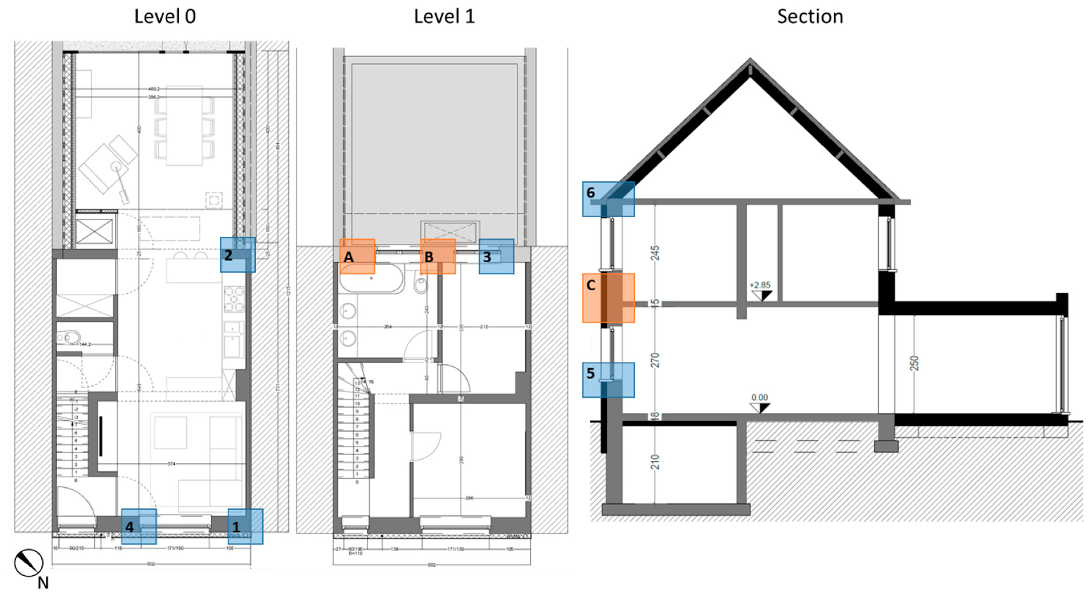
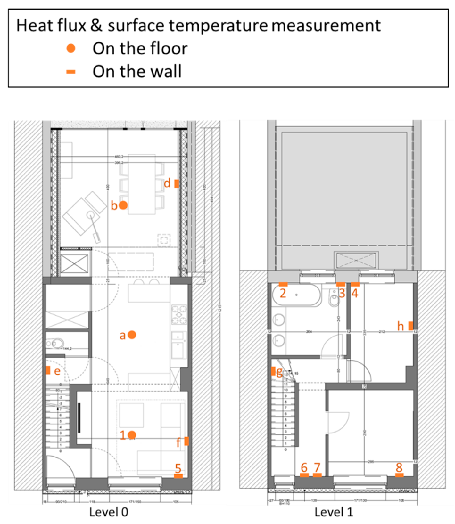
3.3. Performed Measurements

To assess the building envelope performance of the dwelling, co-heating tests [14] and heat flux tests [24] were carried out.

Table 3. Monitoring campaigns.

Test	Start	Stop	Duration	Measurement	Tint,set	Text,mean	Measurement Locations (Figure 5)
Post-retrofit 1	2016-02-16	2016-03-08	21 days	Co-heating test	21.5 °C	3.7 °C	1, 2, 5
Post-retrofit 2	2016-10-26	2016-11-21	26 days	Co-heating test	24.0 °C	7.0 °C	1, 5, 6
Post-retrofit 3	2018-11-15	2018-12-18	33 days	Heat flux test	Variable	5.2 °C	3, 4, 6, 7, 8

summarizes the performed tests, their duration, the indoor temperature setpoint T_int,set, the mean outdoor temperature T_ext,mean and the locations where the heat flux through the building component and accompanying surface temperature were measured, as shown in Figure 5. In this figure, the locations for which the thermal resistance will be identified are numbered, while all other locations are indicated with a letter, representing heat fluxes towards the ground (a and b), towards the cellar (c) and towards the neighboring dwellings (d, e, f, g, and h).

Following the recommendations of previous research [22] a large indoor-outdoor temperature difference was pursued by performing the tests in the heating season, and the test durations were chosen well over 14 days. The post-retrofit dwelling was tested three times: two co-heating tests in unoccupied state and one heat flux test in an occupied state. In between these two co-heating tests, the air tightness of the dwelling was improved. Table 3 shows that the setpoint temperature of the second co-heating test was higher; this value was chosen because of higher outdoor temperatures. Moreover, the indoor set tempereature T_int,set was variable for post-retrofit test 3, because the dwelling was occupied. Hence, the indoor temperature was chosen by the inhabitants. In the three post-retrofit monitoring campaigns, not all indicated heat fluxes were monitored simultaneously (see measurement locations in Table 3). During the final heat flux test (post-retrofit test 3) the fluxes with a letter in Figure 5 were not measured. Note that all heat fluxes were measured on the inside of the building envelope and that there were no mechanical ventilation systems operational during the tests.

Besides these co-heating tests and heat flux tests, pressurization tests were carried out following NBN EN 13829:2001 [60] in order to determine the infiltration losses of the dwelling. In these tests, the infiltration rate is derived from the airflow rate needed to maintain an indoor-outdoor pressure difference of 50 Pa over the building envelope. Additionally, air leaks and thermal bridges were localized in the building envelope by means of infrared scans.

For all measurement campaigns, the outdoor climate was measured at two nearby weather stations located at 2.5 km and 13.5 km distance from the case study, where the following parameters were monitored: outdoor temperature (°C), air pressure (hPa), relative humidity (%), wind direction (°), wind speed (km/h), rainfall (mm/h) and global horizontal irradiation (W/m²).

The accuracy of all used monitoring sensors is summarized in

Table 4. Sensor specifications.

Parameter	Sensor	Unit	Accuracy	Test
Indoor air temperature	Eltek PT100	°C	±0.25 °C	Coheating
Outdoor air temperature	Davis Vantage Pro 2	°C	±0.50 °C	Coheating
Heating power	Elster A100C	A	±1% of the measured value	Coheating
Global horizontal irradiation	Davis solar radiation sensor (6450)	W/m2	±5% of the measured value	Coheating
Flux	Hukseflux HFP01	W/m2	±3% of the measured value	Coheating and Heat flux
Surface temperature	Thermocouple type T	°C	±1.00 °C	Heat flux

.

4. Results

4.1. Building Scale

This section assesses the post-retrofit performance of the case by means of the HLC. First, the theoretical HLC will be derived, which is secondly compared to the resulting measured HLC’s identified by co-heating test. Finally, the sensitivity analysis of the theoretical HLC will illustrate the limitations of the standard calculation methods by assessing the impact of a varying infiltration rate, thermal bridges, and heat exchange through the party walls.

4.1.1. Theoretical Overall Heat Loss Coefficient

The theoretical transmission heat losses H_tr (calculated with Equations (1)–(4), see Section 3.1.1) are summarized in

Table 5. Transmission heat losses towards the exterior.

Building Component	Pre-Retrofit Htr [W/K]	Post-Retrofit Htr [W/K]
Windows and doors	40.8	19.8
Front facade	22.3	4.6
Rear facade	18.4	1.3
Rear facade extension	43.3	1.2
Pitched roof	36.8	8.5
Flat roof extension	60.3	4.5
Old floor on the ground	26.9	10.8
New floor on the ground	-	4.2
Floor above cellar	13.4	5.02
TOTAL	262.2	59.9

. As a result of the retrofit, the theoretical transmission heat losses towards the exterior and adjacent unheated spaces (i.e., the cellar) decreased from 262.2 W/K to 59.9 W/K, which corresponds to a 77% reduction. The windows and doors have the largest share in the post-retrofit transmission heat losses (33%), although also the floor on the ground has a significant impact (25%) because this is the only uninsulated component.

Next, the default infiltration heat losses H_inf are calculated using Equation (5) in Section 3.1.1. This results in an infiltration rate of 0.74 1/h for the post-retrofit state, which leads to an infiltration HLC of 61 W/K. Additionally, the infiltration heat losses can also be calculated for the target value of the post-retrofit infiltration rate, which was 0.20 1/h (see Section 2. Description of the case study). Hence, the target value of the infiltration heat losses is 16 W/K.

Overall, the default theoretical HLC, the sum of the transmission and infiltration HLC, is 127.6 for the post-retrofit state of the dwelling, while the target value of the post-retrofit state is 75.9 W/K.

4.1.2. Measured Overall Heat Loss Coefficient

Two co-heating tests were performed, from which two HLC’s could be identified by means of the ARX-model. For the first post-retrofit test, the identified measured HLC is 206.5 W/K with a standard deviation of 14.7 W/K, while the measured HLC of the second test is 122.6 W/K with a standard deviation of 6.8 W/K. The difference between these two measured values is significant (83.9 W/K), but still, both measured results are very high compared to the theoretical values. On the one hand, the first value is 61% higher than the default theoretical value and even 172% higher than the target value. On the other hand, the improved value of the second test is corresponding quite well with the default theoretical value (difference of 4%), although it is still 62% higher than the target value. Hence, compared to the default theoretical values the overall building envelope performance is quite bad at first, but after performing measures to improve the airtightness, the performance seems to be quite good. However, as the theoretical reference HLC is an essential parameter in this comparison, its variability, and the difference with the measured value will be further assessed in a sensitivity analysis in the next section.

4.1.3. Sensitivity Analysis of the Theoretical HLC

As a first part of the sensitivity analysis, the results of the heat flows regarding infiltration, thermal bridges, and neighboring zones will separately be presented. Secondly, all these heat flows will be joined together in the overall HLC. The variability of this overall HLC will then be discussed to illustrate the impact of assumptions on the theoretical HLC. Finally, the spread of these theoretical HLC’s will be compared to the measured HLC.

Heat Flow Calculations

First, the infiltration heat losses H_inf are estimated with Equation (5) using the three methods to calculate the infiltration rate n_a (Section 3.1.3). The calculations are only carried out for test 1 and 2 (see Table 3), as the indoor air temperatures of the dwelling were not monitored in test 3, which is a necessary input for the LBNL-method. The resulting infiltration rates and their related heat losses are summarized in

Table 6. Infiltration rates and related heat losses—calculated for different methods.

	Method 1		Method 2		Method 3
Test	na [1/h]	Hinf [W/K]	na [1/h]	Hinf [W/K]	na [1/h]	Hinf [W/K]
Post-retrofit test 1	0.74	61	1.09	89	1.50 ± 0.09	124 ± 7
Post-retrofit test 2	0.74	61	0.45	36	0.51 ± 0.05	42 ± 4

. In this table, method 1 is the theoretical default value that was already used to calculate the default HLC in Section 4.1.1, method 2 is the measured value applying the rule of thumb and method 3 is the LBNL-method. Note that the first two sets of infiltration rates are constant values, while for the LBNL-method the distribution of the infiltration rate is shown as a standard deviation.

Table 6 first shows that the target value of the infiltration rate n_a was not achieved: the measured values (method 2 and 3) are more than three times higher than the aimed value of 0.2 per hour. Furthermore, it also shows that the default infiltration (method 1) can deviate significantly from the measured infiltration rates. These deviations can mostly be ascribed to the fact that the default theoretical infiltration rate only incorporates the building envelope area and not its state or airtightness level. This results in the same default infiltration rate for the two post-retrofit tests (since the building envelope area was not changed in between), while the measured value improved due to the applied airtightness measures. Additionally, there is also a difference between the two measured values of method 2 and 3: the results of method 3 are 17% up to 39% higher than these of method 2.

In addition to the infiltration heat losses, six thermal bridges were simulated: four horizontal sections (blue nodes 1 to 4 in Figure 1) and two vertical sections (blue nodes 5 and 6 in Figure 1) through the building envelope. The thermal bridges with the highest linear thermal transmittance (Ψ) are number 1 and 4 (with a heat loss of 1.8 and 1.7 W/K), both horizontal sections in the front facade, while thermal bridge 6—the connection between the front facade and the pitched roof—has the least influence (heat loss of 0.3 W/K). The total heat losses due to thermal bridging effects are 6.69 W/K, which can be considered as an insignificant heat loss compared to the heat losses of transmission (Table 5) and infiltration (Table 6).

Finally,

Table 7. Transmission heat losses towards the neighboring heated dwellings on the left-hand side (L) and the right-hand side (R) of the assessed case study.

Test	Neighboring Zone	A [m2]	Tn,min [°C]	Tn,mean [°C]	Tn,max [°C]	Htr,in,min [W/K]	Htr,in,mean [W/K]	Htr,in,max [W/K]
Post-retrofit test 1	Dayzone L	35.3	20.9	22.7	23.8	1.3	−4.4	−7.8
	Nightzone L	31.4	12.1	16.6	20.1	25.6	13.1	3.3
	Dayzone R	35.3	17.3	19.1	21.2	12.6	6.9	0.3
	Nightzone R	31.4	13.3	19.7	19.7	22.3	11.7	4.5
Post-retrofit test 2	Dayzone L	35.3	20.9	22.7	23.8	10.0	4.2	0.7
	Nightzone L	31.4	12.1	16.6	20.1	34.2	21.3	11.2
	Dayzone R	35.3	17.3	19.1	21.2	21.7	15.9	9.1
	Nightzone R	31.4	13.3	19.7	19.7	30.8	19.8	12.4

shows the heat losses to the neighboring zones (H_tr,in calculated with Equation (9)) at the left (L) and the right (R) of the case study dwelling, split into a day-zone and a night-zone. Due to missing information on the temperatures during test 3, the H_tr,in-value could again only be calculated for test 1 and 2 (see Table 3).

In Table 7, the mean, minimum and maximum value of the neighboring air temperatures, estimated from the surface temperatures measured during the pre-retrofit test (see Section 3.1.2), are shown to assess the variability of the heat exchange with the neighboring dwellings. Since Equation (9) uses the ratio of the temperature difference as a correction factor, the heat losses in Table 7 are only influenced by the indoor temperatures. Consequently, the mean heat losses towards the neighboring dwellings are higher for test 2, with the highest indoor set temperature of 24 °C (Table 3). Table 7 further shows that the variation of the heat losses varies significantly during the tests: for low neighboring temperatures the heat losses H_tr,in,min increase to max. 34.2 W/K per zone, while for high neighboring temperatures H_tr,in,max is negligible for several zones. Therefore, these results show the importance of correcting the heating power ${\mathsf{\varphi }}_h$ for the heat exchange with the neighboring dwellings ${\mathsf{\varphi }}_{tr,n}$ in Equation (6) when the HLC is identified by in situ measurements. If this correction is not carried out, the measured HLC depends on the indoor temperature in the dwelling and its neighbors and hence on the occupant heating behavior.

Impact on the Building Envelope Performance

The overall HLC aggregates all four elements previously discussed: the transmission heat losses, the infiltration heat losses, the thermal bridges, and the heat exchange with the neighboring dwellings. The resulting theoretical HLC varies significantly, depending on the method to define the infiltration rate (Table 6), which thermal bridges are incorporated and whether the heat exchange through the party walls is considered or not (Table 7). Figure 6 compares the range of theoretical HLC’s to the measured values, derived from co-heating test data using ARX-models. A distinction has been made between the HLC without or with heat exchange through the party walls.

Overall, Figure 6 shows that calculating the theoretical HLC is not straightforward: assumptions on the infiltration rate and heat exchange through the party walls have a significant impact on the calculated theoretical HLC. Hence, it seems that it is not evident to identify one value as the theoretical HLC. For both post-retrofit states, the default HLC is strongly deviating from the other theoretical HLC’s for which the measured infiltration rates were used. For post-retrofit state 1, the theoretical HLC can be up to 55% higher than the default HLC, while for post-retrofit state 2 the theoretical HLC can be up to 20% lower. If the heat exchange through the party walls is additionally incorporated, the variability of the theoretical HLC increases even more (from 70 W/K to 131 W/K for post-retrofit state 1 and from 25 W/K to 89 W/K for post-retrofit state 2). The impact of thermal bridges, however, is for this case quite insignificant, as these only increase the default HLC by 5%.

The graph further shows that the correspondence between the theoretical and measured HLC is strongly influenced by the large distribution of the theoretical values. More specifically, the theoretical HLC calculated as the summation of the heat losses by transmission, thermal bridges, and infiltration estimated with the LBNL method has the best correspondence with the measured HLC for the first post-retrofit state. The difference between the theoretical and the measured value is then only 4% and 1% without and with heat exchange through the party walls. Moreover, the difference with the measured HLC is maximal for the default HLC for the first post-retrofit state (difference of 38%), while it is minimal for the second post-retrofit state (difference of 4%). The maximum difference between the theoretical and measured HLC is only 18% for the second post-retrofit state without party walls but increases to 40% if the party walls are incorporated. Overall, quite good correspondence is found between the theoretical and measured HLC if the party walls are not incorporated and the infiltration heat losses are calculated with the LBNL-method; the difference is then a maximum of 15%.

Furthermore, the difference in HLC without or with heat exchange through the party wall is the largest for the second post-retrofit state, both for the theoretical and measured HLC. If the heat losses through the party walls are incorporated, the average HLC increases with 56% for the theoretical and with 30% for the measured value, while for the first post-retrofit state it only increases with 8% and 4% respectively. This illustrates the importance of coping with party wall losses when the overall insulation level increases. Overall, incorporating the heat losses through the party walls does not seem to influence the difference between the theoretical and measured performance on building scale.

4.2. Component Scale

In the previous section the building envelope performance on building scale was discussed. It was shown that various assumptions might cause a large variability of the theoretical HLC. However, the theoretical and measured HLC match quite well for some sets of assumptions (difference of less than 5%, see Figure 6). The current section will now focus on the performance on a component scale. To do so, the thermal resistance of the building components will be evaluated. In addition, the possible causes of the difference between the theoretical and measured thermal resistances are assessed and the limitations of the calculations methods are illustrated. To this end, the robustness of the measured thermal resistances is evaluated, and three building components will be simulated (A, B, and C localized in Figure 1). These simulations will also illustrate the impact of built-in ventilation ducts, a non-homogeneous assembly and air leaks.

4.2.1. Theoretical Thermal Resistance

The theoretical thermal resistances for the tested building components (R_T) are calculated taking into account an uncertainty interval and disregarding the surface resistances, as previously discussed in Section 3.2.1. For the pre-retrofit facades, the theoretical thermal resistance was limited to a maximum 0.69 m²K/W. This poor resistance was improved considerably by the retrofit: for the front facade to a value between 4.76 and 5.39 m²K/W, while the new rear facade improved to values between 8.06 and 8.91 m²K/W. This thermal resistance, however, is only an average value, since the theoretical thermal resistance locally varies significantly, as indicated in Figure 2: R_insul is 9.62 m²K/W, while R_wood is only 4.04 m²K/W and R_HVAC varies with the temperature inside the ventilation duct (see simulations of component A and B in Section 4.2.3). Finally, the estimated thermal resistance of the post-retrofit insulated floor to the cellar lies between 3.77 and 4.17 m²K/W.

4.2.2. Measured Transmission Thermal Resistance

Table 8. Measured thermal resistances.

Component	RT [m2K/W]	Test	Location (Figure 5)	RM [m2K/W]	Range
Insulated floor to Cellar	3.77–4.17	Post-retrofit test 2	1	3.77	0.69
Rear facade	8.06–8.91	Post-retrofit test 1	2	4.85	0.98
Rear facade	8.06–8.91	Post-retrofit test 3	3	6.63	1.16
Front facade	4.76–5.39	Post-retrofit test 1	5	1.19	0.30
Front facade	4.76–5.39	Post-retrofit test 2	5	1.26	0.51
Front facade	4.76–5.39	Post-retrofit test 2	6	2.70	1.42
Front facade	4.76–5.39	Post-retrofit test 3	6	3.08	3.47
Front facade	4.76–5.39	Post-retrofit test 3	7	8.65	45.37
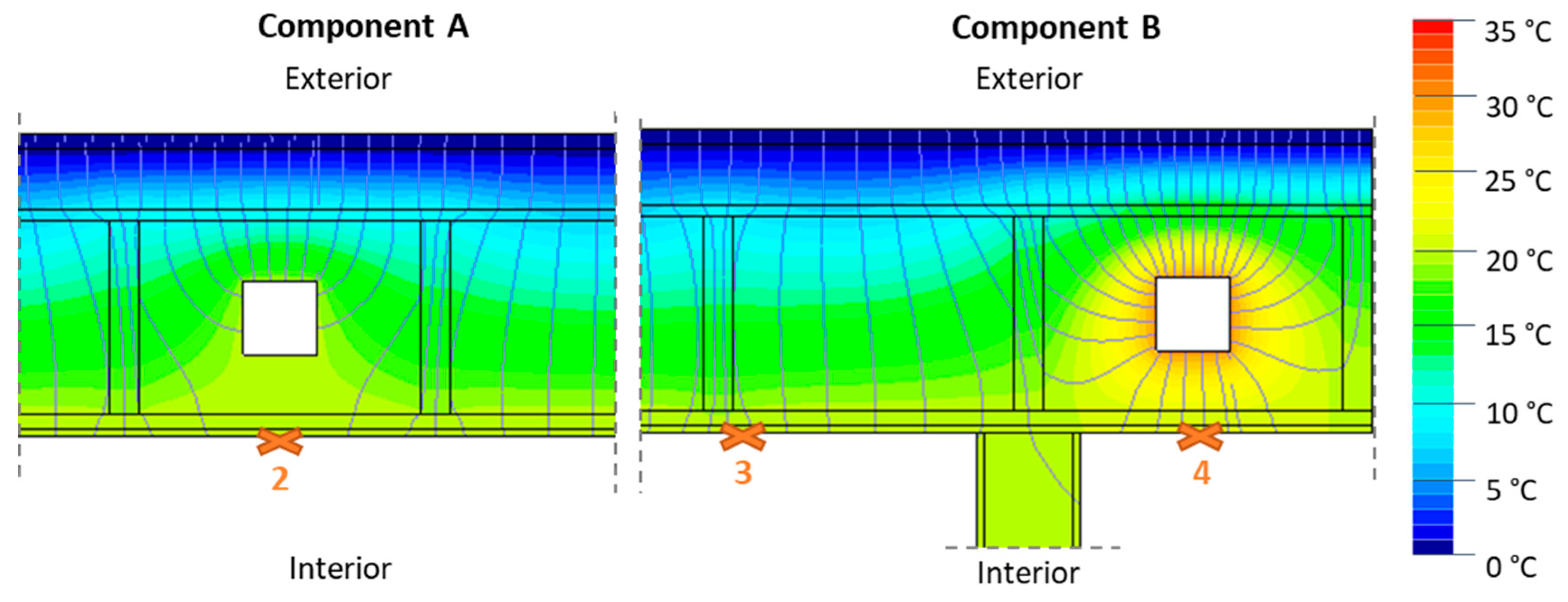
Front facade	4.76–5.39	Post-retrofit test 3	8	1.65	1.34

summarizes the thermal resistances identified from the measurements on three building components following Anderlinds’ regression method (Equation (10)). It shows the theoretical thermal resistances (R_T), the performed tests (Table 3), the tested location (Figure 5), the measured thermal resistance, and the range expressing the robustness of the identified thermal resistance.

First, Table 8 shows that the theoretical thermal resistance of the insulated floor is achieved, although the range is quite high (0.69 m²K/W corresponds with an 18% variation of the average value).

The second building component of which the results are shown in Table 8 is the rear facade. The two identified thermal resistances at post-retrofit locations 2 and 3 (shown in Figure 5) on the wall are 22% and 43% lower than the theoretical value, while for post-retrofit location 4 no thermal resistance could be derived at all. After performing post-retrofit test 3, detailed design plans were collected, showing the complete assembly of the prefabricated rear facade. This additional information located some inhomogeneities that could explain the large range of the measured thermal resistances shown in Table 8: Post-retrofit location 2 was found to be close to a built-in ventilation duct, which serves as an air outlet, post-retrofit location 3 was found to be nearby the wooden studs, which is a local thermal bridge and finally post-retrofit location 4 was close to a built-in ventilation duct, which serves as a warm air supply duct. The impact of these inhomogeneities will be illustrated by means of the simulations of components A and B, which will be discussed in Section 4.2.3.

The third building component shown in Table 8 is the front facade. For this component, all measured results are strongly deviating from the theoretical thermal resistance: five results are more than 40% lower, while, in contrast, one result is 67% higher. Additionally, the range of post-retrofit measurement location 7 is extremely high (more than 45 m²K/W). A possible explanation for these results could be variable air in- or exfiltration in the cavity, explaining the significant variation of the measured thermal resistances. Warm interior air infiltrating the cavity can increase the apparent thermal resistance of a building component, while cold exterior air can decrease it. To assess this hypothesis, simulations were carried out using Delphin, modeling the heat flux through the front facade for different infiltration rates of the air cavity. These simulations are discussed in the next section for component C.

Next, Table 8 also shows the range of the thermal resistances, which is considerably high for location 7 at the front facade (maximum value of 45.37 m²K/W). Since low ranges indicate that the identified thermal resistance is quite constant for sequential subsets of the data, this suggests that dynamic phenomena influencing the instantaneous thermal resistance, for instance fluctuating temperatures, solar radiation or wind pressures, are not captured by the Anderlinds’ regression model with a 24 h influence time (Equation (10)). Moreover, for all measurements, the range is higher than 17% of the identified thermal resistance.

Overall, we can conclude from Table 8 that only for one out of nine measurements the measured thermal resistance corresponds with the theoretical value.

4.2.3. Simulations

This section presents the simulation results in two parts. In the first part, the heat flux simulations of the building components will be presented, in order to verify the hypotheses that were previously raised on the cause of the deviation between the theoretical and measured thermal resistances. In the second part, the airflow simulations of component C will be discussed, which illustrates the limitations of the calculation and characterization methods.

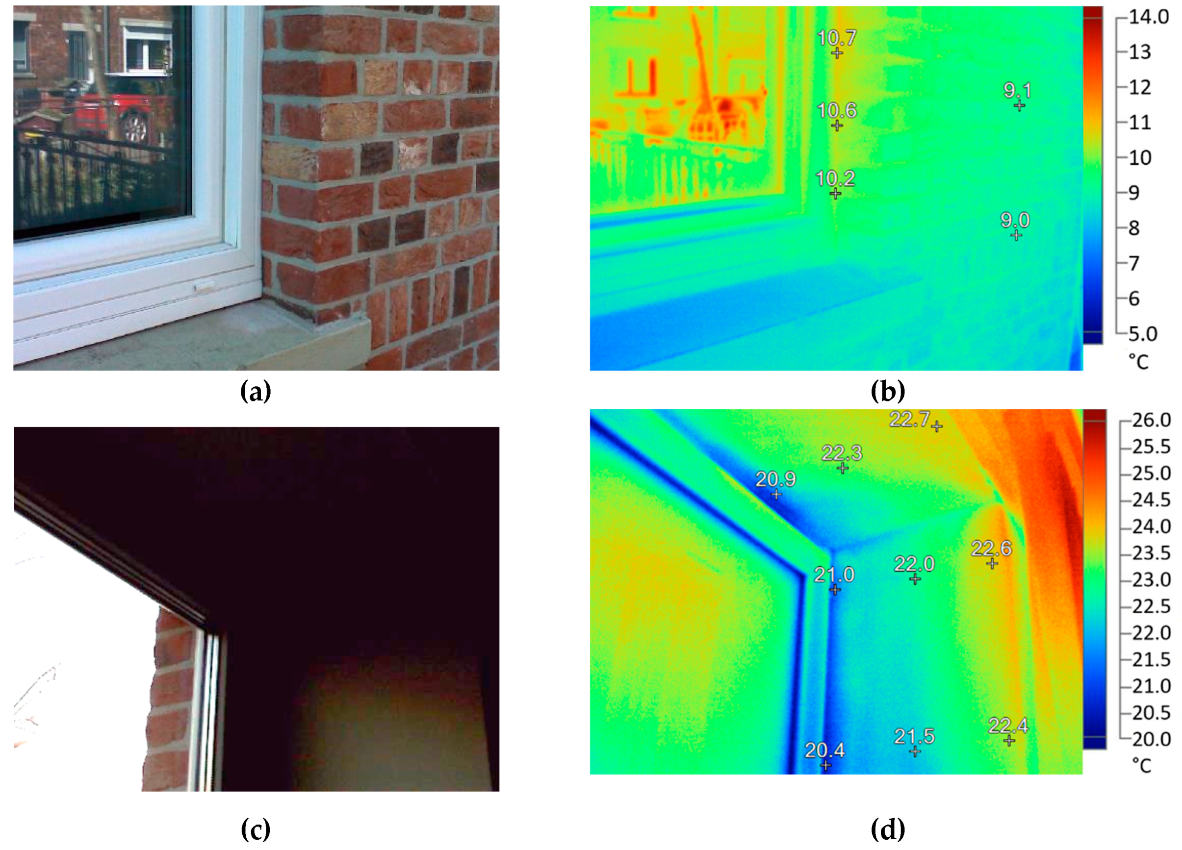
Heat Flux Simulations

To verify whether the nonhomogeneous assembly of the post-retrofit rear facade is the cause of the differences between the theoretical and measured thermal resistances for the three measurement locations shown in Table 8, a heat transfer simulation was performed with TRISCO. The simulated heat transfer of nonhomogeneous components A and B (located in Figure 1) are illustrated in Figure 7, which shows the simulated temperature distribution and isoflux-lines. Additionally, the post-retrofit measurement locations 2, 3, and 4 are also indicated, with the presence of an air outlet at location 2, a wooden stud at location 3, and a warm air inlet at location 4. Firstly, both the air outlet and inlet have a significant impact on the temperature variance and the heat flux pattern, although the impact of the warm air inlet is the highest. Based on the simulation results, both ventilation ducts seem to induce an increase in internal temperature in the building component, although this increase is significantly higher for the air inlet at location 4. Next, the wooden stud mainly seems to have an impact on the heat flux pattern: The heat flux towards the exterior is locally higher here, while the temperature distribution is only slightly disturbed.

In order to assess whether the very high measured thermal resistance shown in Table 8 for measurement location 7 (situated in Figure 5) could be a result of air cavity infiltration, building component C is simulated (situated in Figure 1 and visualized in Figure 3). Figure 8 shows the simulation results from Delphin [55,56], illustrating the temperature distribution in the insulated front facade as a result of two types of air cavity ventilation: cold exterior or warm interior air infiltration (ACH = 80 1/h). The plots show that the simulated airflow particularly influences the temperature of the two brick slabs of the original wall: cold air infiltration easily decreases the inner surface temperature with 5 °C.

These heat flux simulations of the building components show that construction details such as a nonhomogeneous assembly or air cavity flows have a significant impact on the heat fluxes and temperatures in building components. Since these two parameters were measured during the heat flux measurements, both the nonhomogeneous assembly and the air cavity flows could have influenced the measured thermal resistances. It should be emphasized, however, that other phenomena could have influenced the measurements as well.

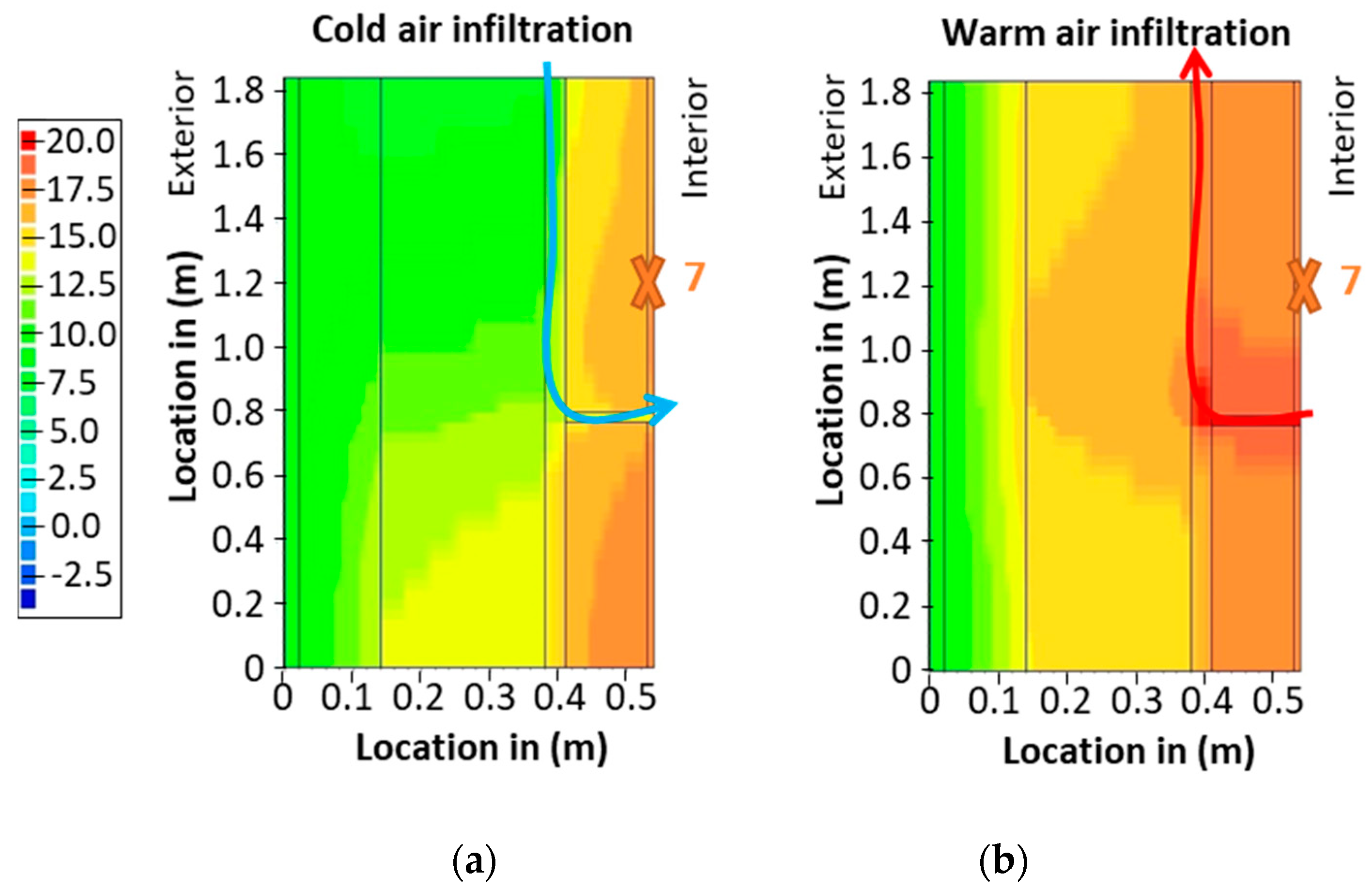
Air Flow Simulations (Component C)

The high range of 45.4 m²K/W at post-retrofit measurement location 7 (Table 8), indicates that the characterization model of this location is not robust. To explain this very high range, as well as to identify why the model couldn’t capture a robust thermal resistance, various air cavity flows are simulated for component C.

First, the moving window analysis from which the range is derived is visualized on the top graph of Figure 9. This graph shows subsequent thermal resistances identified for a 10-day subset of the data: each identified thermal resistance is shown on this graph on the moment when the ten days subset of the dataset starts. For example, the first thermal resistance shown on the graph on the 18th of November is identified for a subset of the data from the 18th to the 28th of November. The large variation of the thermal resistance shown on this graph is the cause of the large range: Starting from the 25th of November, the thermal resistance increases to the maximum value of 46.5 m²K/W on the 30th of November, to decrease again afterward.

Because high thermal resistances are induced by low heat fluxes from the interior to the exterior (Equation (10)), the variation of the measured heat flux in time is shown on the middle graph of Figure 9 (in green), together with the simulated heat fluxes depending on the ventilation rate of the cavity. The simulated heat fluxes resulting from cold exterior air infiltrating in the cavity, induced by positive air change rates (ACH 0 to 160), are visualized in blue (left phenomenon illustrated in Figure 8). The fluxes resulting from warm interior air infiltrating in the cavity, induced by negative air change rates (ACH −160 to 0) are visualized in red (right phenomenon illustrated in Figure 8). A negative heat flux indicates heat losses towards the outside, while a positive heat flux indicates heat gains from the outside. The measured heat flux, visualized in green, illustrates that for the first part of the data, quite high heat losses were measured (values lower than −7.5 W/m²), leading to the low estimated thermal resistances in the first part of the top graph of Figure 9. Subsequently, the middle part of the data (1st till 12th of December) shows that the heat losses are very low (lower than −2.5 W/m²), with even some periods of heat gains. Estimating the thermal resistance of the wall only for this part of the data leads to the high values visualized on the top graph of Figure 9.

The middle graph of Figure 9 also shows that for the middle part of the data, the measured heat flux corresponds with the simulated heat fluxes resulting from warm interior air infiltrating the cavity. For the remaining parts of the data, the measured heat flux corresponds with the simulated heat fluxes resulting from cold exterior air infiltrating the cavity, although there are still some measured fluxes that have higher values than the simulated fluxes. In order to find an explanation for the strong variation in heat flux, the main driving forces for air infiltration are plotted in the bottom graph of Figure 9. These driving forces are the wind pressure and the pressure resulting from thermal stack effects, calculated for the front facade with Equations (11)–(14).

Only at moments when the measured negative heat flux exceeds the simulated values, the wind pressure on the facade is positive, which causes the cold air to infiltrate in the cavity. Furthermore, moments when heat gains are measured coincide with the lowest values for the wind pressure. These observations gave the incentive to check the correlation between the measured heat fluxes and the wind pressure. Overall, a moderate correlation of 0.68 was found. This suggests that air cavity flows caused by wind pressures influence the heat flux through the facade and hence also the thermal resistance of the post-retrofit front facade. The correlation with the stack pressure, however, is rather weak (−0.39), and also no visual correlation can be derived from Figure 9.

To assess whether all measured thermal resistances of the post-retrofit front facade are similarly influenced by air cavity ventilation as illustrated in Figure 8 and Figure 9 the correlation coefficient between the fluxes (W/m²) measured at four locations for the front facade and the simulated wind pressures (P_w in Pa) are summarized in

Table 9. Correlation between the measured heat fluxes (q) and wind pressure (P_w) on the post-retrofit front facade.

Description	Post-Retrofit Test 1	Post-Retrofit Test 2		Post-Retrofit Test 3
Location (Figure 5)	5	5	6	6	7	8
Measured thermal resistance	1.19	1.26	2.70	3.08	8.65	1.65
Correlation q~Pw	0.46	0.16	0.24	0.65	0.68	0.58
Time Pw > 0	19.1%	12.5%		30.1%
Time −2 < Pw < 0	70.1%	82.7%		57.4%
Time Pw < −2	10.8%	4.8%		12.5%

. Surprisingly, there is a lot of variation of the correlation coefficients between the measured heat flux and wind pressure for the different tests: The correlation is weak for post-retrofit test 1 (0.46) and very weak for post-retrofit test 2 (0.16 and 0.24). The strongest correlation was found for post-retrofit test 3 (0.58, 0.65, and 0.68). It is observed that these correlations can be linked to the variance of wind pressure in time. Therefore, Table 9 also shows the percentage of the measurement period that wind pressure P_w on the front facade was positive, between −2 Pa and 0 Pa (generating a weak under pressure) and lower than −2 Pa (generating a strong under pressure). For post-retrofit test 2, which has the weakest correlation with wind pressures, the wind generates a moderate under pressure for 82.7% of the time, lying between −2 Pa and 0 Pa. Next, for post-retrofit test 1, with a slightly higher correlation, there is a moderate under pressure for only 70.1% of the time, and finally, for post-retrofit test 3 the under pressure is moderate for only 57.4% of the time. Hence, wind pressure has a greater impact on the heat flux variation if the pressure is rather extreme (positive or lower than −2). For moderate under pressures, however, the measured thermal resistance is less varying (lower model error, see Table 8), but still 50% up to 75% lower than the theoretical thermal resistance.

5. Discussion

Some recommendations regarding the identification of the building envelope performance can be formulated from the presented results. On building scale, the heat exchange through the party walls was found to incorporate a high degree of uncertainty in the theoretical HLC. Hence, if the heat losses through party walls should be identified, we advise performing sufficient additional measurements (e.g., the heat flow towards the neighboring dwellings, or the temperature in the neighboring dwellings). Besides the heat exchange through the party walls, the infiltration heat losses also induce a large variability of the theoretical HLC. A maximum deviation of 48% was found between the default infiltration heat losses and the measured values. Therefore, a pressurization test should be performed to estimate the infiltration heat losses and assess the HLC correctly. On a component scale, it is very important to get acquainted with the air leaks and inhomogeneities of a building envelope, prior to performing any heat-flux tests. This can be achieved for example by gathering design plans of the building, or by performing a pressurization test combined with an infrared scan. Moreover, the identification of one static thermal resistance is unlikely to represent the performance of a full building component, as it might be strongly influenced by local inhomogeneities. Therefore, the tests should be performed on multiple measurement locations per building component. As for the methods used to identify the thermal resistances, assessing different subsets of the data was illustrated to be a useful method to evaluate large variations of the measured thermal resistances. The periods with extreme apparent thermal resistances could then be identified and subsequently, the cause of these extreme values could be assessed.

Besides these recommendations, the impact of the differences between the theoretical and measured thermal resistances on the theoretical HLC can be estimated. To do so, the theoretical UA-values of the walls can be recalculated, using the measured U-values instead of the theoretical ones (see Table 1 and Table 5). This increases the transmission heat losses with 6.2 W/K (9%) for the post-retrofit dwelling, which induces an overall increase of the theoretical HLC’s with maximum 6%. This increase improves the correspondence between the theoretical and measured HLC if the party walls are not incorporated (see Figure 6). It should be noted, however, that only the walls and part of the floor of the dwelling are assessed; measuring the thermal resistance of the other building components may further influence the HLC.

6. Conclusions

By comparing the theoretical and measured envelope performance of the post-retrofit building envelope of a case study, this paper aimed to illustrate the limitations of the calculation and characterization methods. To this end, the impact of standardized boundary conditions and construction imperfections regarding the building envelope was assessed. First, the building envelope was evaluated on building scale by identification of the theoretical and measured HLC. To identify the measured HLC, a model was implemented following the guidelines of the IEA EBC Annex 58 and Annex 71. Next, the uncertainty of the theoretical HLC caused by infiltration, thermal bridges, and heat exchange through party walls was estimated. Second, the building envelope was evaluated on a component scale and hypotheses on the cause of the difference between the measured and theoretical thermal resistances were tested by simulations.

On building scale, the results show that the correspondence between the theoretical and measured HLC strongly depends on how the theoretical HLC is defined, as the difference between the theoretical and measured HLC varied between 15% and 40%. Assumptions on the infiltration rates and the heat exchange through party walls have a strong influence on the identification of the theoretical HLC. If the heat exchange through the party walls was disregarded and the infiltration heat losses were defined by the LBNL-model, the difference between the theoretical and measured HLC’s was the least. Using measured infiltration rates instead of default values changed the default HLC with up to 55% and 20% for the two post-retrofit states of our case study. Incorporating the heat exchange through the party walls increased the spread of the theoretical HLC even more (increase with a factor 1.9 and 3.5 for the two post-retrofit states).

On a component scale, a poor correspondence between theoretical and measured thermal resistances was found, as only one out of nine measurements match the theoretical values (Section 4.2.2). Simulations illustrated that the measurements could have been influenced by local inhomogeneities or internal airflows. These complex phenomena are difficult to incorporate in theoretical calculations on the one hand and characterization models to identify the measured performance on the other hand. To illustrate these limitations, the thermal resistance of the externally insulated front facade was evaluated, for which the influence of air cavity ventilation caused by wind pressure was assessed.

The comparison of the theoretical and measured building envelope performance revealed a contradiction between a relatively good correspondence on building scale and a poor correspondence on a component scale. This contradiction illustrates that the complexity of the building envelope performance is difficult to capture, which makes it insufficient to only assess the overall envelope performance to explain the energy performance gap. Moreover, the relation between the heat losses and the energy use of a dwelling is not unambiguous and can be influenced by several other factors that are not assessed in this paper, such as the impact of occupant behavior and the performance of the building services.

In conclusion, evaluation of the building envelope underlined that both the theoretical and measured building envelope performance should be identified and interpreted with caution. Several additional measurements, such as a pressurization test, an infrared scan, and assessing the heat losses towards neighboring dwellings, are recommended in order to correctly evaluate the impact of shortcomings and boundary conditions of the building envelope prior to performing co-heating tests or heat flux tests.

References

1. European Commission. Communication from the Commission to the European Parliament, The European Council, the European Economic and Social Committee, the Committee of the Regions and the European Investment Bank. A Clean Planet for All. A European Strategic Long-Term Vision Fo. COM 2018, 773, 1–25. [Google Scholar]
2. European Commission; Eurostat. Final Energy Consumption by Sector. Available online: https://ec.europa.eu/eurostat/tgm/refreshTableAction.do?tab=table&plugin=1&pcode=ten00124&language=en (accessed on 30 January 2020).
3. The European Parliament; The Council of the European Union. Directive 2010/31/EU of the European Union and the Counsil, on the Energy Performance of Buildings. Off. J. Eur. Union 2010, 334, 13–35. [Google Scholar]
4. The European Parliament; The Council of the European Union. Energy Performance of Buildings Directive, Amending Directive 2010/31/EU on the Energy Performance of Buildings and Directive 2012/27/EU on Energy Efficiency. Off. J. Eur. Union 2018, L156, 75–91. [Google Scholar]
5. Eurostat Statistics Explained. People in the EU—Statistics on Housing Conditions. Available online: https://ec.europa.eu/eurostat/statistics-explained (accessed on 1 November 2019).
6. Hens, H.; Parijs, W.; Deurinck, M. Energy Consumption for Heating and Rebound Effects. Energy Build. 2010, 42, 105–110. [Google Scholar] [CrossRef] [Green Version]
7. Calì, D.; Osterhage, T.; Streblow, R.; Müller, D. Energy Performance Gap in Refurbished German Dwellings: Lesson Learned from a Field Test. Energy Build. 2016, 127, 1146–1158. [Google Scholar] [CrossRef]
8. Majcen, D.; Itard, L.C.M.; Visscher, H. Theoretical vs. Actual Energy Consumption of Labelled Dwellings in the Netherlands: Discrepancies and Policy Implications. Energy Policy 2013, 54, 125–136. [Google Scholar] [CrossRef]
9. De Wilde, P. The Gap between Predicted and Measured Energy Performance of Buildings: A Framework for Investigation. Autom. Constr. 2014, 41, 40–49. [Google Scholar] [CrossRef]
10. La Fleur, L.; Moshfegh, B.; Rohdin, P. Measured and Predicted Energy Use and Indoor Climate before and after a Major Renovation of an Apartment Building in Sweden. Energy Build. 2017, 146, 98–110. [Google Scholar] [CrossRef] [Green Version]
11. Gupta, R.; Kapsali, M. Evaluating the “as-Built” Performance of an Eco-Housing Development in the UK. Build. Serv. Eng. Res. Technol. 2016, 37, 220–242. [Google Scholar] [CrossRef]
12. Kuusk, K.; Kalamees, T.; Link, S.; Ilomets, S.; Mikola, A. Case-Study Analysis of Concrete Large-Panel Apartment Building at Pre- and Post Low-Budget Energy-Renovation. J. Civ. Eng. Manag. 2017, 23, 67–75. [Google Scholar] [CrossRef]
13. Bell, M.; Wingfi, J.; Miles-Shenton, D.; Seavers, J. Low Carbon Housing Lessons from Elm Tree Mews; Joseph Rowntree Foundation: York, UK, 2010; pp. 1–118. ISBN 978-1-85935-766-8. [Google Scholar]
14. Wingfield, J.; Johnston, D.; Miles-Shenton, D.; Bell, M. Whole House Heat Loss Test Method (Coheating); Centre for the Built Environment: Leeds, UK, 2010. [Google Scholar]
15. Delghust, M. Improving the Predictive Power of Simplified Residential Space Heating Demand Models: A Field Data and Model Driven Study; Ghent University: Gent, Belgium, 2016. [Google Scholar]
16. Khoury, J.; Alameddine, Z.; Hollmuller, P. Understanding and Bridging the Energy Performance Gap in Building Retrofit. Energy Procedia 2017, 122, 217–222. [Google Scholar] [CrossRef]
17. Ali, Q.; Thaheem, M.J.; Ullah, F.; Sepasgozar, S.M.E. The Performance Gap in Energy-Efficient Office Buildings: How the Occupants Can Help? Energies 2020, 13, 1480. [Google Scholar] [CrossRef] [Green Version]
18. Kaminska, A. Impact of Heating Control Strategy and Occupant Behavior on the Energy Consumption in a Building with Natural Ventilation in Poland. Energies 2019, 12, 4304. [Google Scholar] [CrossRef] [Green Version]
19. Bergman, T.L.; Lavine, A.S.; Incropera, F.P.; Dewitt, D.P. Fundamentals of Heat and Mass Transfer, 7th ed.; John Wiley & Sons, Inc.: New York, NY, USA, 2011. [Google Scholar]
20. Ahmad, N.; Ghiaus, C.; Thiery, T. Influence of Initial and Boundary Conditions on the Accuracy of the QUB Method to Determine the Overall Heat Loss Coefficient of a Building. Energies 2020, 13, 284. [Google Scholar] [CrossRef] [Green Version]
21. Senave, M.; Roels, S.; Verbeke, S.; Lambie, E.; Saelens, D. Sensitivity of Characterizing the Heat Loss Coefficient through On-Board Monitoring: A Case Study Analysis. Energies 2019, 12, 3322. [Google Scholar] [CrossRef] [Green Version]
22. Bauwens, G. Situ Testing of a Building’s Overall Heat Loss Coefficient. Embedding Quasi-Stationary and Dynamic Tests in a Building Physical and Statistical Framework; KU Leuven: Leuven, Belgium, 2015. [Google Scholar]
23. Bureau for Standardisation (NBN). NBN EN ISO 6946:2007—Building Components and Building Elements—Thermal Resistance and Thermal Transmittance—Calculation Method (ISO 6946:2007); NBN: Brussels, Belgium, 2008; pp. 1–40. [Google Scholar]
24. International Organization for Standardization (ISO). ISO 9869-1:2014. Thermal Insulation—Building Elements—In-Situ Measurement of Thermal Resistance and Thermal Transmittance—Part 1: Heat Flow Meter Method; ISO: Vernier, Switzerland, 2014; pp. 1–44. [Google Scholar]
25. Deconinck, A.-H. Reliable Thermal Resistance Estimation of Building Components from On-Site Measurements; KU Leuven: Leuven, Belgium, 2017. [Google Scholar]
26. Bureau for Standardisation (NBN). NBN EN 12831:2003. Heating Systems in Buildings—Method for Calculation of the Design Heat Load; BIN: Brussels, Belgium, 2003; pp. 1–79. [Google Scholar]
27. Blomsterberg, Å.; Carlsson, T.; Svensson, C.; Kronvall, J. Air Flows in Dwellings—Simulations and Measurements. Energy Build. 1999, 30, 87–95. [Google Scholar] [CrossRef]
28. Prignon, M.; Van Moeseke, G. Factors Influencing Airtightness and Airtightness Predictive Models: A Literature Review. Energy Build. 2017, 146, 87–97. [Google Scholar] [CrossRef]
29. Wingfield, J.; Miles-Shenton, D.; Bell, M. Evaluation of the Party Wall Thermal Bypass in Masonry Dwellings; Leeds Metropolitan University: Leeds, UK, 2009; pp. 1–6. [Google Scholar]
30. Lowe, R.J.; Wingfield, J.; Bell, M.; Bell, J.M. Evidence for Heat Losses via Party Wall Cavities in Masonry Construction. Build. Serv. Eng. Res. Technol. 2007, 28, 161–181. [Google Scholar] [CrossRef]
31. Senave, M. Characterization of the Heat Loss Coefficient of Residential Buildings Based on In-Use Monitoring Data; KU Leuven: Leuven, Belgium, 2019. [Google Scholar]
32. Gupta, R.; Dantsiou, D. Understanding the Gap between ‘as Designed’ and ‘as Built’ Performance of a New Low Carbon Housing Development in UK. In Sustainability in Energy and Buildings; Hakansson, A., Höjer, M., Howlett, R.J., Jain, L.C., Eds.; Smart Innovation, Systems and Technologies; Springer: Berlin/Heidelberg, Germany, 2013; Volume 22, pp. 567–580. [Google Scholar] [CrossRef]
33. Delghust, M.; Janssens, A.; Rummens, J. Retrofit Cavity-Wall Insulation: Performance Analysis from in-Situ Measurements. In Proceedings of the 1st Central European Symposium on Building Physics (CESBP 2010), Cracow, Poland, 13–15 September 2010. [Google Scholar]
34. Madsen, H.; Bacher, P.; Bauwens, G.; Deconinck, A.-H.; Reynders, G.; Roels, S.; Himpe, E.; Lethé, G. Thermal Performance Characterization Using Time Series Data—IEA EBC Annex 58 Guidelines. IEA EBC Annex 2015, 58, 83. [Google Scholar]
35. Platform for Renovation. Platform for Renovation: Pilot Project Mutatie +. Available online: https://www.kennisplatform-renovatie.be/proeftuinprojecten/mutatie/ (accessed on 20 November 2019).
36. Bureau for Standardisation (NBN). NBN B 62-002. Thermische Prestaties van Gebouwen—Berekening van de Warmtedoorgangscoëfficiënten (U-Waarden) van Gebouwcomponenten En Gebouwelementen—Berekening van de Warmteoverdrachtscoëfficiënten Door Transmissie (HT-Waarde) En Ventilatie (Hv-Waarde); NBN: Brussels, Belgium, 2008; pp. 1–215. [Google Scholar]
37. European Committee for Standardization (CEN). ISO/CD 13370. Thermal Performance of Buildings—Heat Transfer via the Ground—Calculation Methods. Revision of ISO 13370:1998; ISO: Vernier, Switzerland, 2004; pp. 1–56. [Google Scholar]
38. Flemish Government. Bijlage V—Bepalingsmethode EPW. Bepalingsmethode van Het Peil van Primair Energieverbruik van Residentiële Eenheden; Flemish Government: Brussels, Belgium, 2018; pp. 1–216.
39. Snyder, R.L. Hand Calculating Degree Days. Agric. For. Meteorol. 1985, 35, 353–358. [Google Scholar] [CrossRef]
40. Jankovic, L. Improving Building Energy Efficiency through Measurement of Building Physics Properties Using Dynamic Heating Tests. Energies 2019, 12, 1450. [Google Scholar] [CrossRef] [Green Version]
41. Kurnitski, J.; Saari, A.; Kalamees, T.; Vuolle, M.; Niemelä, J.; Tark, T. Cost Optimal and Nearly Zero (NZEB) Energy Performance Calculations for Residential Buildings with REHVA Definition for NZEB National Implementation. Energy Build. 2011, 43, 3279–3288. [Google Scholar] [CrossRef]
42. Olofsson, T.; Andersson, S. Overall Heat Loss Coefficient and Domestic Energy Gain Factor for Single-Family Buildings. Build. Environ. 2002, 37, 1019–1026. [Google Scholar] [CrossRef]
43. Szodrai, F.; Lakatos, Á.; Kalmár, F. Analysis of the Change of the Specific Heat Loss Coefficient of Buildings Resulted by the Variation of the Geometry and the Moisture Load. Energy 2016, 115, 820–829. [Google Scholar] [CrossRef] [Green Version]
44. Kronval, J. Testing of Houses for Air Leakage Using a Pressure Method. ASHRAE Trans. 1978, 84, 72–79. [Google Scholar]
45. Awbi, H.B. Ventilation of Buildings, 2nd ed.; Spon Press, Taylor & Francis Group: London, UK; New York, NY, USA, 2003. [Google Scholar] [CrossRef]
46. International Organization for Standardization (ISO). ISO 10211:2007. Thermal Bridges in Building Construction—Heat Flows and Surface Temperatures—Detailed Calculations; ISO: Vernier, Switzerland, 2007; pp. 1–54. [Google Scholar]
47. Werkgroep PAThB2010. Gevalideerde Numerieke Berekeningen; PAThB2010: Brussels, Belgium, 2009. [Google Scholar]
48. Physibel. TRISCO, Computer Program to Calculate 3D & 2D Steady State Heat Transfer in Rectangular Objects; Physibel: Ghent, Belgium, 2019. [Google Scholar]
49. Belgisch staatsblad—Moniteur Belge. Transmissiereferentiedocument; Flemish Government: Brussels, Belgium, 2010; pp. 74848–74936.
50. Anderlind, G. Multiple Regression Analysis of in Situ Thermal Measurements—Study of an Attic Insulated with 800 Mm Loose Fill Insulation. J. Therm. Insul. Build. Envel. 1992, 16, 81–104. [Google Scholar] [CrossRef]
51. International Organization for Standardization (ISO). EN ISO 10077-2: Thermal Performance of Windows, Doors and Shutters—Calculation of Thermal Transmittance—Part 2: Numerical Method for Frames (ISO 10077-2:2017); ISO: Vernier, Switzerland, 2017; p. 70. [Google Scholar]
52. Physibel. TRISCO & KOBRU86. Computer Program to Calculate 3D & 2D Steady State Heat Transfer in Rectangular Objects; Version 12.0w; Physibel: Ghent, Belgium, 2010; pp. 1–108. [Google Scholar] [CrossRef]
53. Lambie, E.; Saelens, D. The Thermal Resistance of Retrofitted Building Components Based on In-Situ Measurements. In Proceedings of the 7th International Building Physics Conference IBPC2018, Syracuse, NY, USA, 23–26 September 2018; pp. 959–964. [Google Scholar]
54. Maroy, K.; Steeman, M.; Van Den Bossche, N. Air Flows between Prefabricated Insulation Modules and the Existing Façade: A Numerical Analysis of the Adaption Layer. Energy Procedia 2017, 132, 885–890. [Google Scholar] [CrossRef]
55. Bauklimatik Dresden. Delphin Simulation Software; Institute for Building Climatology at Dresden University of Technology (Faculty of Architecture): Dresden, Germany, 2019. [Google Scholar]
56. Nicolai, A.; Grunewald, J. Delphin 5 Version 5.2 User Manual and Program Reference; Institute for Building Climatology at Dresden University of Technology (Faculty of Architecture): Dresden, Germany, 2006. [Google Scholar]
57. Langmans, J.; Desta, T.Z.; Alderweireldt, L.; Roels, S. Field Study on the Air Change Rate behind Residential Rainscreen Cladding Systems: A Parameter Analysis. Build. Environ. 2016, 95, 1–12. [Google Scholar] [CrossRef] [Green Version]
58. Vanpachtenbeke, M.; Langmans, J.; Roels, S.; Van Acker, J. Modelling Cavity Ventilation behind Brick Veneer Cladding: How Reliable Are the Common Assumptions? Energy Procedia 2015, 78, 1467–1477. [Google Scholar] [CrossRef] [Green Version]
59. Liddament, M. AIVC Guide to Energy Efficienct Ventilation; The Air Infiltration and Ventilation Centre: Coventry, UK, 1996; pp. 1–274. [Google Scholar]
60. Bureau for Standardisation (NBN). NBN EN 13829:2001. Thermal Performance of Buildings—Determination of Air Permeability of Buildings—Fan Pressurization Method; BIN: Brussels, Belgium, 2001; pp. 1–25. [Google Scholar]
Figure 1. Floor plans of the case study with six thermal bridges indicated in blue (see Section 3.1.2 and Section 4.1.1) and three simulated building components in orange (see Section 3.2.2 and Section 4.2.3)—measures in cm.
Energies 13 02469 g001
Figure 2. Horizontal section of the post-retrofit rear facade, component A and B.
Energies 13 02469 g002
Figure 3. Vertical section of the post-retrofit front facade at component C.
Energies 13 02469 g003
Figure 4. Infrared scan of the building. Top: Air leaks around the window frames connecting the outside and the air cavity—seen from the outside with the building under positive pressure. (a) Exterior photo and (b) Infrared image. Bottom: Air leaks around the window frames connecting the outside and the air cavity – seen from the inside with the building under negative pressure. (c) Interior photo and (d) Infrared image.
Energies 13 02469 g004
Figure 5. Monitoring campaigns: Sensor locations for the post-retrofit state of the dwelling.
Energies 13 02469 g005
Figure 6. Theoretic and measured heat loss coefficients.
Energies 13 02469 g006
Figure 7. Simulation of the temperature variance and isoflux-lines of the post-retrofit rear facade by means of TRISCO.
Energies 13 02469 g007
Figure 8. Simulation of the temperature variance for air cavity ventilation in the front facade. (a) Cold exterior air infiltrating in the cavity. (b) Warm interior air infiltrating in the cavity.
Energies 13 02469 g008
Figure 9. Assessment of the measured thermal resistance and heat flux for measurement location 7. Top: Estimated thermal resistance for a moving window of 10 days along the dataset, each time shifting with 1 h. Middle: Simulated heat fluxes vs. measured heat flux. Bottom: Simulated wind pressure and thermal stack pressure on the front facade.
Energies 13 02469 g009