Abstract
This paper introduces a new protection system for solar photovoltaic generator (SPVG)-connected networks. The system is a combination of voltage-restrained overcurrent relays (VROCRs) and directional overcurrent relays (DOCRs). The DOCRs are implemented to sense high fault current on the grid side, and VROCRs are deployed to sense low fault current supplied by the SPVG. Furthermore, a novel challenge for the optimal coordination of DOCRs-DOCRs and DOCRs-VROCRs is formulated. Due to the inclusion of additional constraints of VROCR, the relay coordination problem becomes more complicated. To solve this complex problem, a hybrid Harmony Search Algorithm-Bollinger Bands (HSA-BB) method is proposed. Also, the lower and upper bands in BB are dynamically adjusted with the generation number to assist the HSA in the exploration and exploitation stages. The proposed method is implemented on three different SPVG-connected networks. To exhibit the effectiveness of the proposed method, the obtained results are compared with the genetic algorithm (GA), particle swarm optimization (PSO), cuckoo search algorithm (CSA), HSA and hybrid GA-nonlinear programming (GA-NLP) method. Also, the superiority of the proposed method is evaluated using descriptive and nonparametric statistical tests.
1. Introduction
As fossil fuel reserves are depleting, the price and related environmental concerns strongly encourage the use of renewable energies [1,2,3]. The solar photovoltaic generator (SPVG) is one of the premier alternatives to fossil fuels that generates AC from DC power by using inverters. However, the response of SPVG to grid faults is more or less controllable by the power electronics used in an inverter system [1]. Thus, this difference has to be considered when designing a protective system for SPVG-connected networks [4].
In a network without distributed generators (DGs), directional overcurrent relays (DOCRs) are a suitable choice for the protection systems because of their ease in functionality and cost-effectiveness. In the last decade, a range of evolutionary algorithms and their hybrid approaches have become recognized as a means for solving the coordination problem of DOCRs [5,6,7,8,9,10,11].
Overcurrent-based protective systems have shown their effectiveness for conventional power systems, but this has been changing gradually due to the rising inclusion of DGs and power electronic devices. Inverters used in SPVG, because of the low thermal overload capability, are actively current limited and have a small current contribution (1.2 to 1.5 times the normal current in the grid fault condition) [1,12]. As a result, the overcurrent protection for the grid-connected configuration appears to take more fault clearing time. The responsive characteristics of overcurrent relay are essential for addressing this, but they are not endurable for a protection scheme. Protecting the inverter-dominated DGs such as SPVGs is, therefore, a challenging technical issue.
To address this issue, an inverse time admittance (ITA) relay, which is independent of current, has been used for an inverter-interfaced DGs (IIDGs)-connected network to sense and remove faulty section under low or changing fault current levels [13]. Major concerns for applications of ITA relay are the measurements of the admittance for short lines, fault resistance, and harmonic and transient behavior of current.
In [14], the frequency-based protection scheme is shown by using anti-islanding frequency relays. A significant issue with this scheme is that it is not practical to assume that all relays can be replaced [15].
Fault current limiter (FCL), another advanced technique, is used to limit the fault current supplied by DGs during grid fault. It restores the original settings of DOCRs [16,17,18]. However, the mutual influence of DGs makes it problematic, considering the impedance value of the FCL for a high level of DG penetration. The switching losses are also a major issue with this approach [16,19]. Hence, this approach is not suitable for increasing installations of SPVG with maximum capacities.
As IIDGs are a good resource of harmonics, a protection system based on the harmonic injection is proposed [20]. In this scheme, harmonics are injected into the network during a fault. Protection relays are used to observe and disconnect the inverter if the total harmonic distortion of terminal voltage exceeds the threshold value during a fault. This technique may fail when the numbers of dynamic loads are present. Furthermore, protection schemes with an advance communication infrastructure—e.g., adaptive relaying [21], communication-assisted digital relays [22], a phasor measurement units-assisted integrated impedance angle based scheme [23], or a microgrid central protection unit [15]—can effectively solve protection issues in an SPVG-connected network. However, the cost involved in their communication infrastructure and for updating the existing protection devices cannot justify these choices. Also, the risk of failing communication channels and threats of cybersecurity are an issue for employing these protective systems [24].
The different protection schemes [25,26] are used in a micro-grid, having synchronous and inverter-based DGs. The problems of communication cost and its failure, unbalanced loads, transients during connection and disconnections of DGs are associated with these schemes. While using energy storage devices such as the flywheel and batteries, the fault current can be increased at desired levels, letting the overcurrent relays to work traditionally [27,28]. Conversely, this method requires a significant investment and correct maintenance for safe operation. Recently, non-standard characteristics-based protection schemes were suggested for microgrid protection [29,30,31]. These types of characteristics provide flexibility in the operation of relays, but the complexity of the mathematical expressions and extra controlling parameters are challenging issues [32]. Overall, these solutions are not adequate for increasing installations of SPVG with maximum capacity.
As discussed in [33,34], the inverters and the point of common coupling (PCC) of the grid-connected SPVG system are perturbed by grid fault condition. It is rare but possible that the damage of SPVG is caused by an accident in the distribution network where most SPVGs are connected. Most damages resulting from faults in the distribution network can be protected by the inverters installed in the SPVG. However, if this protection fails, the central inverter installed in the SPVG will be damaged.
If the inverter installed in the SPVG (central inverter or string inverter) fails, the generation of the entire SPVG is stopped. For example, in South Korea, if an inverter of 1 MW SPVG fails, power generation stops for a period of two to four weeks, and the expected generation revenue during that period (in case of 4.8 h/day generation) is 67.2 to 134.4 MWh of electricity [3,35]. In order to connect a SPVG system to the grid, a set of devices of protection are provided at PCC. This protection system performs the appropriate functions to prevent the SPVG feeds the network in case of abnormal values of current, voltage and frequency.
This paper:
- demonstrates that to develop a reliable protection scheme for SPVG-connected networks, voltage-restrained overcurrent relays (VROCRs) are deployed to sense a low fault current on the SPVG side, whereas DOCRs are used to operate with a high fault current on the grid side. VROCRs can sense a low fault current by providing the set overcurrent operating value in proportion to the applied input voltage. Also, VROCRs helps to maintain grid stability because they can avoid unnecessary isolations of SPVG networks against short-term disturbances such as voltage dips due to the fault cleared by DOCRs.
- formulates a new problem of optimum coordination of DOCRs-DOCRs and DOCRs-VROCRs in SPVG-connected networks.
- hybridizes the Harmony Search Algorithm (HSA) with the Bollinger Bands (BB) approach for accelerating a local search and improving the convergence and accuracy of the results. The BB method is also modified to support HSA in exploration and exploitation.
- estimates the performance of the proposed hybrid approach by applying over three case studies. The outcomes in terms of the total operating time, violations in constraints, and convergence behaviour are compared with the genetic algorithm (GA), particle swarm optimization (PSO), cuckoo search algorithm (CSA), HSA and hybrid GA-nonlinear programming (GA-NLP) methods.
- performs a statistical analysis using descriptive and nonparametric tests to demonstrate the more excellent value of HSA-BB.
2. Problem Formulation of Optimum Relay Coordination
In the optimum coordination of relays, the foremost objective is to obtain relay settings that minimize the total operating time of relays under the coordination and boundary constraints. The objective function and the constraints formulation for optimum relay coordination are shown in the following sub-sections.
2.1. Objective Function (OF)
The OF, which needs to be minimized, is the sum of the operation times of relays when they act as primary relays [6].
where TOPi indicates the time of the primary relay Ri, and k shows the number of primary relays.
2.2. Constraints
The desired constraints in the relay coordination problem should be satisfied while minimizing the OF. These constraints are formulated as follows.
2.2.1. Coordination Time Interval (CTI)
The time interval between the operating time of primary and backup (P/B) protection is essential for preserving selectivity. Its time interval is known as CTI, and it may be stated as:
where tb and tp are the operation of times in the order of backup and primary relays.
2.2.2. Bounds on Relay Settings
The DOCR has only two settings of the current pickup setting (Ipi) and time multiplier setting (TMS), whereas VROCR has an additional third setting of voltage pickup setting (Vpi).
The bounds on TMS of the relay may be defined as:
TMS range can be represented as a continuous value from 0.1 to 1.1 for DOCRs [5] and 0.05 to 1.1 for VROCRs [36].
The boundaries of Ipi of a relay can be presented as:
To ensure the security and reliability of protection schemes [6,7], Ipi is determined based on two parameters, the maximum full-load current and lowest fault current.
The boundaries of Vpi of the relay may be defined as:
The fault in the power network is attended by a related voltage dip, while the overload causes an only modest drop in voltage. Therefore, a voltage and current measurement-based fault detection relay—such as VROCR—can discriminate between overload and fault. VROCR becomes increasingly responsive to overcurrent as the voltage of the systems drops [37]. The Vpi range can be taken as a continuous value from 0% to 85% of the system nominal voltage.
2.2.3. Bounds on Time of Operation (TOP) of Relay
A certain minimum amount of operating time is needed for a relay. It should not take a long operating time. This constraint is defined as:
where TOPmin and TOPmax are the minimum and maximum operating times of the relay.
2.2.4. Characteristic of Relay
The inverse definite minimum time (IDMT) characteristic for DOCRs is widely used in the protection system [5,6,7,8,9,10,11]. It is defined as follows.
where If is the fault current.
Based on the IEC 60255-3 standard, a VROCR characteristic is expressed as [36]:
where V and I are the measured values of voltage and current by VROCR. Ipi and Vpi are the pickup settings of the current and voltage of VROCR, respectively.
3. Hybrid HSA-BB Method
The proposed hybrid HSA-BB approach is illustrated in this section. In the following sub-sections, a brief introduction of the HSA and BB is shown before explaining the hybridization of HSA-BB.
3.1. Harmony Search Algorithm
The HSA is a successful metaheuristic algorithm introduced by Geem et al. [38]. It is stimulated by the ideologies of the musicians’ improvisation process for finding the best harmony. The flowchart for HSA is represented in Figure 1.
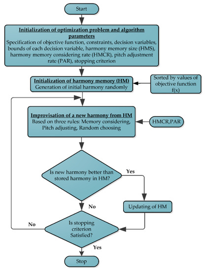
Figure 1.
Flow diagram of the Harmony Search Algorithm (HSA).
The HSA can be executed in the following stages [8,38,39,40,41].
Step 1: Initialize the optimization problem and parameters of the algorithm:
For the HSA application, the OF with constraints and decision variables should be initialized as:
where is the objective function, P and M represent the numbers of constraints, P (equality), and M (inequality). xi shows the decision variables set, and N is the number of variables. The upper and lower boundaries for decision variables are represented in the order of xi,U, and xi,L. In this step, the algorithm parameters (i.e., harmony memory size (HMS), harmony memory consideration rate (HMCR), pitch adjustment rate (PAR)), and a maximum number of iterations are also provided. All solution vectors are stored in the harmony memory (HM). Solution vectors are improvised using HMCR and PAR, as demonstrated in step 3.
Step 2: Initialize the HM:
In this step, the randomly generated solution vectors (x1, …, xHMS) are stored in the HM, according to HMS. It is defined by the following equation.
It is possible that infeasible solutions with violated constraints arise. When this occurs, the algorithm forces the search towards a feasible solution area using the static penalty function.
Step 3: Generate a new harmony by improvising the stored harmony in the HM:
A new vector of harmony is formed according to the HMCR, PAR, and a random selection, which is called improvisation. According to the HMCR, ith variable of can be improvised using Equation (11). HMCR is the probability of selecting a value from the stored value in the HM, whereas (1-HMCR) is the probability of randomly generating a new value. The range of HMCR is defined between 0 and 1.
If xi’ is selected from the HM, it is further tuned using PAR. PAR represents the probability of a component from the HM mutating, while (1-PAR) shows the probability of no mutation. It is expressed using the following equation.
where rand [0, 1] represents the randomly generated value in the range of 0 and 1. bw is the bandwidth of arbitrary distance for the design variable.
Step 4: Update the HM:
If, according to the OF value, a newly generated vector is better than the worst one that existed in the HM, the worst should be replaced by a new one.
Step 5: Check the criterion for stopping the algorithm:
Step 3 and step 4 are repeated until a stopping criterion (e.g., maximum numbers of iteration) has been met.
3.2. Bollinger Bands Approach
The Bollinger Bands method is widely used to forecast the upcoming prices of the stocks. It was developed by J. Bollinger [42]. Based on historical data, it computes the mean and standard deviation of the prices for estimating the interval. The BB for each decision variable can be premeditated using the following terms.
The mean is considered as a middle band and can be calculated for decision variable xi as:
where n is the number of available samples of each variable.
The standard deviation for decision variable xi is calculated as:
For decision variable xi, the upper and lower bands are calculated using the following expression.
where UBi and LBi are the upper and lower bands. a is the constant value and selected in the range of 1 to 2.
Further, the xi is updated by the following equation.
where xi’ is a newly generated value for variable x, and r is a randomly generated value between 0 and 1.
3.3. Hybrid HSA-BB Method
Exploration and exploitation are important parameters for metaheuristic methods. Exploration parameters ensure that algorithms will not be biased in local optima. Exploitation parameters exploit previous solutions for reducing the randomization, which ultimately helps the algorithm in faster convergence. Very strong exploitation can cause the slowing down of the exploration, which ultimately leads to premature convergence and an insignificant solution. To deal with this issue and to develop a more efficient algorithm, different search strategies are hybridized in the literature [6,7,9,39,43]. Similarly, the HSA is useful for exploring to find nearby global regions, but it has a problem of searching the local optima [39]. On the other hand, BB has good exploiting history, since it utilizes all previous components while generating new ones. Therefore, in this study, the HSA is hybridized with BB to enhance the performance of HSA in terms of a local search, accuracy of results, and convergence. Also, BB is modified to help the HSA in exploration during the initial generation and in exploitation during the final generation. The HSA and BB are hybridized as follows.
1. Adaptive Bollinger band: The value of a when calculating the upper and lower bands in BB is illustrated by Equations (15) and (16), and fixed between 1 and 2. However, a higher value of a can cause a larger gap between the upper and lower bands, and a lower value of a makes this gap smaller. From Equation (17), it is clear that during the early generations, smaller gaps will provide smaller values when updating the current value of the component (xi), which ultimately affects exploration. However, any algorithm should be good at exploring during early generations, so that it may not be trapped in local optima. On the other hand, during final generations, a larger gap will provide a larger value while updating the current component (xi), which ultimately affects the exploitation. As discussed earlier, weak exploitation slows down the convergence performance of algorithms. To deal with this problem, the parameter a in Equations (15) and (16) is modified such a way that it dynamically changes with each generation. It is shown by the following equation.
where NI represents the maximum number of iterations, whereas gn shows the generation number.
2. Using Equation (12), HSA performs a local search. This equation is modified using Equation (17) of BB. Initially, the HSA completes the course search by using randomization and HMCR and fills the HM. Using the solution vectors stored in the HM, BB calculates the mean and standard deviation as well as the lower and upper bands for each decision variable as given by Equations (13)–(16). It is also noted that the number of samples n is equal to the HMS. Suppose that HMS is considered as 30, then the available number of sample values of each decision variable is 30. Afterward, a new value for each decision variable is computed by Equation (17) of BB in the local search step of HSA (Equation (12) in step 3). This is illustrated as follows.
If the new solution vector of decision variables is better than the worst one stored in the HM, then the worst vector is replaced with new one. The remaining steps of the proposed hybrid approach are the same as the HSA, which is already discussed in Section 3.1.
4. Simulation Results and Discussion
The performance of a proposed hybrid HSA-BB approach for the optimal coordination of DOCRs-DOCRs and DOCRs-VROCRs is verified on SPVGs connected-three different power networks. The first test case has 14 DOCRs and 1 VROCR, the second has 24 DOCRs and 4 VROCRs, and the third has 78 DOCRs and 3 VROCRs. The SPVG is designed based on the data given in [1,35,44,45,46]. ETAP software is used for modeling and fault calculation of SPVG-connected networks. Ranges of TMS are considered in all cases, from 0.1 to 1.1 for DOCRs and 0.05 to 1.1 for VROCRs, respectively. The minimum time of operation of each relay and CTI are assumed in order of 0.2 and 0.3 s for test cases 1 and 2. Both are considered to be 0.2 s in test case 3. Simulation outcomes are compared with GA, PSO, CSA, HSA, and GA-NLP for demonstrating the effectiveness of the HSA-BB. The comparative study is conducted in terms of convergence behavior and statistical analysis for an IEEE 30-bus system. The parameter values for all algorithms are given in Table 1.

Table 1.
Parameter values of all algorithms for each test system.
4.1. Case 1: 8-Bus Network
The proposed hybrid approach is implemented on a 40 MW SPVG-connected eight-bus network with a voltage rating of 150 kV. A minimum rating of 40 MW is required for SPVG if it is connected to the high voltage grid of 132 kV or above [1]. Accordingly, the 40 MW SPVG is designed, and it supplies 150 A current to the eight-bus network through bus 5, as shown in Figure 2. The data for the eight-bus network were provided in [47].
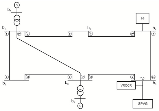
Figure 2.
Diagram of SPVG-connected 8-bus system.
Table 2 lists the results of the current magnitude for close-in 3-Φ fault current and P/B DOCRs pairs. Table 3 contains the voltage and current sensed by VROCR for a close-in fault to each DOCR. It is learned from Table 3 that VROCR senses the maximum fault current (1.45 times the rated current supplied by SPVG) for the close-in fault to relays 5 and 11. The voltage drop (0% of system nominal voltage) is also maximum in this case. Similarly, the minimum fault current (1.15 times the rated current supplied by SPVG) and voltage drop (20.42 % of system nominal voltage) are sensed by VROCR for the close-in fault to relays 1 and 13. As shown in Figure 3, the VROCR trips for the current above 110% of the full load current supplied by SPVG, and voltage drops below 85% of the system nominal voltage. The voltage sensed by VROCR is 0 kV for the close-in fault to relays 5 and 11. The characteristic of VROCR presented by Equation (8) becomes undefined. Hence, the maximum value of 20 is assumed for in Equation (8) for the close-in fault to relay 5 and 11 in this case.
Table 2.
Fault current for primary and backup (P/B) directional overcurrent relays (DOCRs) pairs of 8-bus network.
Table 3.
Measured quantities by VROCR for the close-in fault to each DOCR of 8-bus network.
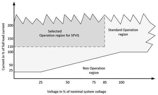
Figure 3.
Voltage-restrained overcurrent relay (VROCR) operating characteristics based on pickup settings of current and voltage for SPVG protection.
By implementing all methods, the obtained results of relay settings, TOP of primary relays, and OF value formed by using Equation (1) are displayed in Table 4. HSA-BB provides the best minimized OF (9.636 s) compared to hybrid GA-NLP (9.795 s), HSA (12.325 s), CSA (12.533 s), PSO (14.417 s) and GA (16.916 s). The CTI between P/B DOCRs-DOCRs and DOCRs-VROCR is tabulated in Table 5. As seen from this result, the CTI is maintained at a minimum level (0.3 s) for almost all P/B DOCRs-DOCRs pairs in HSA-BB as compared to other stated methods. The CTI of P/B DOCRs-VROCR pairs is also minimal in HSA-BB as compared to other methods. As the HSA-BB gives better results than other employed methods, further analysis of VROCR operation is discussed only for the results obtained by HSA-BB.
Table 4.
Results of 8-bus network.
Table 5.
Coordination time interval (CTI) values of P/B relay pairs for 8-bus system.
For the close-in fault to relay 5 and 11, the CTI of relay pairs 5-VROCR and 11-VROCR is 0.745 and 0.583 s, respectively. For the close-in fault to relay 6 and 7, relay 5 operates as the first backup and VROCR as a second backup. The CTI of relay pairs 6-5 and 7-5 are 0.4340 and 0.3 s, respectively. Thus, VROCR should operate after a minimum CTI of 0.7340 s (0.4340 + 0.3) and 0.6 s (0.3 + 0.3) for the close-in fault to relays 6 and 7. As shown in Table 5, VROCR operates after 0.8711 and 0.7371 s for the close-in fault to relays 6 and 7, respectively. In the case of close-in fault to relay 10, relay 11 as the first backup operates after 0.3 s time interval. Therefore, VROCR as the second backup should trip after 0.6 s. However, VROCR operates over a long time of 1.2720 s because VROCR senses less voltage reduction and fault current for the close-in fault to relay 10 than a close-in fault to relay 6 and 7, as shown in Table 3. For the close-in fault to relay 1, 2, and 8, VROCR works as a third backup. The CTI of relay pair 1-VROCR (2.2964 s) is more extensive than relay pairs 2-VROCR (1.0884 s) and 8-VROCR (1.3533 s), since VROCR experiences minimum voltage reduction and fault current for the close-in fault to relay 1 as shown in Table 3. The CTI of relay pair 2-7 (0.3 s) is less than the CTI of relay pair 8-7 (0.5649 s). Thus, VROCR trips over a long time to the close-in fault to relay 8 than the close-in fault to relay 2. For the close-in fault to relay 9, VROCR also works as a third backup and operates over 2.0340 s. This is because it experiences a moderate voltage reduction and fault current compared to relays 1, 2, and 8. With the final results of CTI of DCORs-VROCR, it can be deduced that the operation of VROCR depends on sensing the voltage reduction and fault current supplied by the SPVG as well as its action as backup protection.
4.2. Case 2: 9-Bus Network
In this case, four SPVG-connected systems with nine buses (b1 to b9) are considered (Figure 4). An SPVG of 8–10 MW is required for connecting to a 30–34.5 kV grid [1]. Therefore, each SPVG is designed with ratings of 8 MW and 33 kV. These are connected as SPVG1 at b7, SPVG2 at b5, SPVG3 at b9, and SPVG4 at b3. Each SPVG supplies the current of 138 A to the network. The external grid (EG) with 400-MVA short circuit capacity is connected to b1. The impedance of each line segment is (0.0057 + j0.071) Ω/km. The current magnitude for close-in 3-Φ fault sensed by P/B pairs of DOCRs is provided in Table 6.
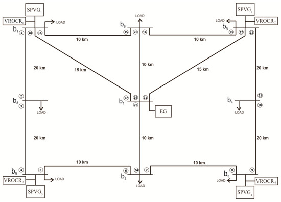
Figure 4.
Diagram of a four SPVG-connected 9-bus system.
Table 6.
Fault current for P/B DOCR pairs of 9-bus system.
Table 7 shows the voltage and current sensed by VROCRs for the close-in fault to each DOCR. It can be seen that maximum fault current and voltage drop are sensed by VROCR1 for the close-in fault to relay 1, 16 and 18, by VROCR2 for the close-in fault to relay 12, 13 and 22, by VROCR3 for the close-in fault to relay 4 and 5, and by VROCR4 for the close-in fault to relay 8 and 9. Similarly, the minimum fault current and voltage drop are experienced by VROCR1 and VROCR3 for the close-in fault to relay 10 and 11, and VROCR2 and VROCR4 for the close-in fault to relay 2 and 3, respectively.
Table 7.
Measured quantities by VROCRs for the close-in fault to each DOCR of the 9-bus network.
Table 8 shows the use of all the approaches, and the results of relay settings, the TOP of primary relays and the OF value. It is seen from Table 8 that the OF value acquired by using HSA-BB is less as compared to GA, PSO, CSA, HSA, and GA-NLP. The CTI value derived for P/B DOCRs-DOCRs and DOCRs-VROCRs pairs for the close-in fault to each DOCR is presented in Table 9 and Table 10, respectively. It is seen in Table 9 and Table 10 that all the coordination constraints have been satisfied when determining the results of these methods. Also, the larger value of CTI shows the larger operating time of backup relays, which is not desirable for a protection system. In Table 9, the obtained value of CTI for P/B DOCRs-DOCRs pairs is almost maintained to the minimum prescribed level in the results of HSA-BB. Also, the fast operating time of VROCR may raise unnecessary isolation of SPVG if it is used as a backup of DOCRs, thus putting grid network stability at risk [1]. As shown in Table 10, the purpose of the larger CTI value for DOCRs-VROCRs pairs (i.e., 10-VROCR1 and 11-VROCR1, 2-VROCR2 and 3-VROCR2, 10-VROCR3 and 11-VROCR3, 2-VROCR4 and 3-VROCR4) is to ride through disturbances for avoiding the undesirable removal of SPVG. Therefore, a less sensitive setting is preferred for the VROCR when it needs to operate as a backup of DOCRs, especially for the far fault to the VROCR.
Table 8.
Results of 9-bus network.
Table 9.
CTI of P/B DOCRs-DOCRs pairs of 9-bus network.
Table 10.
CTI of P/B DOCRs-VROCRs pairs for 9-bus network.
4.3. Case 3: IEEE 30-Bus Network
To confirm the success of the proposed hybrid approach, its performance needs to be demonstrated using a larger and more complex system. For this task, the IEEE 30-bus network is selected, as shown in Figure 5. It can be considered as a meshed sub-transmission and distribution system [10]. This complex power network has 30 buses (132 kV and 33 kV buses), 37 lines, 78 DOCRs and 3 VROCRs. In addition, three SPVGs with the rating of 8 MW are connected to the distribution network (33 kV) as SPVG1 at b19, SPVG2 at b22 and SPVG3 at b23. As it includes VROCRs, the total number of constraints increased to 666 as compared to 426 when considering only DOCRs in the test system. Thus, optimization methods have to consider highly constrained optimization problems in this test case.
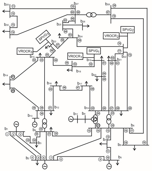
Figure 5.
Diagram of three SPVGs connected IEEE 30 bus network.
Table 11 shows the results obtained by implementing all the methods for the IEEE 30-bus system. It comprises the OF values, numbers of violated coordination constraints, required numbers of iteration, and convergence time. The given OF value by HSA-BB, shown in Table 11, is the minimum compared to all other methods. It is also experienced that during the simulations of this complex system, sometimes hybrid GA-NLP does not converge even at a feasible solution and stops prematurely. Also, a violation of coordination constraints has been observed in GA, PSO, CSA, HSA, and GA-NLP, whereas there is no violation observed in the results of the proposed methods. The convergence of all algorithms is graphically illustrated in Figure 6. As seen in Table 11 and Figure 6, the numbers of iteration and convergence time are also lowest in the HSA-BB method as compared to GA, PSO, CSA, HSA, and GA-NLP methods. The simulation results confirm that HSA-BB gives better results compared to the remaining methods. However, the proposed HSA-BB algorithm has more parameters to be tuned as compared to the other methods. The tuning of the parameters is indeed a time consuming and tedious task. Also, the harmony memory size is bigger than the initially generated nest of the cuckoo search method. Therefore, it requires more memory to store the solutions.
Table 11.
Comparative results for the IEEE 30-bus network.
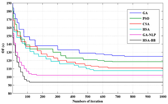
Figure 6.
Convergence to the best objective function (OF) value for IEEE 30-bus network.
Furthermore, a comparative study of all the methods is performed, using descriptive and nonparametric statistical tests. Table 12 shows the results of a descriptive statistical study based on 50 runs. The lower value of standard deviation in the results of HSA-BB indicates that it gives the most predictable results in all 50 runs, compared to other methods. Additionally, because the mean and worst values are very near to the best value, quality results are obtained by HSA-BB.
Table 12.
Descriptive statistical results based on 50 runs for IEEE 30-bus network.
Moreover, paired t-test and Wilcoxon signed-rank tests are widely used to determine the significant difference in the behavior and superiority of algorithms. However, the paired t-test is a parametric test and needs to be certain that the essential conditions are satisfied, i.e., independence, normality [48,49]. The condition of independence is fulfilled because 50 samples of the OF are obtained by 50 simulations of all algorithms with randomly produced initial seeds. Furthermore, samples from different runs were normal when their behavior assisted a normal or Gauss distribution.
The normality of the data is initially examined by the skewness and kurtosis. Skewness and kurtosis are needed to calculate the frequency distribution of data. Skewness helps to recognize the right and left tails of frequency distribution from a central value, while kurtosis gives an idea about the shape and nature of hump of a frequency distribution. The data can be said to be normally distributed when the skewness and kurtosis are equal to 0 and 3, respectively [50]. As seen in Table 12, the normal distribution is not verified from the results of skewness and kurtosis obtained by 50 runs of each algorithm. Hence, the statistical normality tests are further performed by using Anderson–Darling and Kolmogorov–Smirnov tests [48,49]. All the tests determine the p-value, which shows the variation of the sample of results concerning the normal shape. The p-value is less than the level of significance (α = 0.05), indicating the rejections of normality. The results of p-values for all the algorithms by using normality tests are provided in Table 13. From Table 13, it is noted that both tests indicate that none of the outputs of the algorithms give perfect Gaussian distribution. Hence, it is justified to employ a nonparametric test, neglecting the parametric one.
Table 13.
Comparative results of normality tests of all the algorithms.
In this study, the effectiveness of the proposed hybrid algorithm over other algorithms is substantiated using Wilcoxon signed-rank test [48], which is a nonparametric test. In this test, a null hypothesis states that the behavior of algorithms which are compared to each other is similar, whereas an alternative hypothesis states the opposite. If the p-value for the null hypothesis is below the significant level (α = 0.05), this hypothesis is rejected. The sum of rankings and p-value obtained in each comparison of algorithms is given in Table 14. From Table 14, it is seen that the p-value, when compared to HSA-BB with other algorithms, is below 0.05 and confirmed that the HSA-BB behaves differently compared to the remaining algorithms. In Table 14, R+ is the sum of ranks for the data sets on which the first algorithm outperforms the second, and R− is the sum of ranks for the opposite. From Table 14, it is seen that R− is higher in all the comparison of other algorithms with HSA-BB. From the results of the Wilcoxon test, it is deduced that the proposed HSA-BB outperforms the GA, PSO, CSA, HSA, and GA-NLP algorithms with a significant level of 0.05.
Table 14.
Comparative results of the Wilcoxon test of all the algorithms.
5. Conclusions
This study presents a DOCR- and VROCR-based combined protection scheme. In this scheme, the VROCRs are used to operate for a low fault current on SPVG side protection, and DOCRs are implemented to sense a high fault current on grid side protection. This protection methodology provides better fault detection for low fault current contributed by SPVG, and high fault current contributed by the grid. It also avoids unwanted isolation of SPVG in the case of short-term disturbances.
A hybrid HSA-BB method is employed to resolve the unique challenge of optimal coordination of DOCRs-DOCRs and DOCRs-VROCRs on three different SPVG-connected networks. The BB methodology is used in the improvisation stage of HSA. The BB method is also modified to dynamically adjust the gap between upper and lower bands with generation numbers so that it helps HSA in both exploration and exploitation.
For evaluating the capability of the proposed method in solving the relay coordination problem, the obtained results are compared with other well-established methods (GA, PSO, CSA, HSA, and GA-NLP). Outcomes of the comparative analysis validate that a significant reduction in the total operating time of relays is obtained using hybrid HSA-BB without violating the constraints compared to the other methods. In addition, the hybrid HSA-BB method takes minimum iteration to reach the best optimum solution, which reveals that the proposed method is also better in convergence performance. From the descriptive statistical test, it is found that the proposed method gives consistent solutions for different runs, which shows the capability of the proposed method in providing a better-quality solution. Furthermore, the results of nonparametric tests verify the significant difference in behavior as well as the superiority of the hybrid HSA-BB method compared to the other employed methods.
Author Contributions
Conceptualization, V.N.R., K.S.P.; Methodology, V.N.R., K.S.P.; Writing—Original Draft Preparation, V.N.R.; Writing-Review & Editing, Z.W.G., J.H.; Supervision, K.S.P., Z.W.G.; Funding Acquisition, Z.W.G., J.H. All authors have read and agreed to the published version of the manuscript.
Funding
This research was supported by the Energy Cloud R&D Program through the National Research Foundation of Korea (NRF) funded by the Ministry of Science, ICT (2019M3F2A1073164).
Conflicts of Interest
The authors declare no conflict of interest.
References
- Hernández, J.; De la Cruz, J.; Ogayar, B. Electrical protection for the grid-interconnection of photovoltaic-distributed generation. Electr. Power Syst. Res. 2012, 89, 85–99. [Google Scholar] [CrossRef]
- Geem, Z.W. Size optimization for a hybrid photovoltaic–wind energy system. Int. J. Electr. Power Energy Syst. 2012, 42, 448–451. [Google Scholar] [CrossRef]
- Shin, H.; Geem, Z.W. Optimal design of a residential photovoltaic renewable system in South Korea. Appl. Sci. 2019, 9, 1138. [Google Scholar] [CrossRef]
- Cagnano, A.; De Tuglie, E.; Mancarella, P. Microgrids: Overview and guidelines for practical implementations and operation. Appl. Energy 2020, 258, 114039. [Google Scholar] [CrossRef]
- Amraee, T. Coordination of directional overcurrent relays using seeker algorithm. IEEE Trans. Power Deliv. 2012, 27, 1415–1422. [Google Scholar] [CrossRef]
- Bedekar, P.P.; Bhide, S.R. Optimum coordination of directional overcurrent relays using the hybrid GA-NLP approach. IEEE Trans. Power Deliv. 2011, 26, 109–119. [Google Scholar] [CrossRef]
- Noghabi, A.S.; Sadeh, J.; Mashhadi, H.R. Considering different network topologies in optimal overcurrent relay coordination using a hybrid GA. IEEE Trans. Power Deliv. 2009, 24, 1857–1863. [Google Scholar] [CrossRef]
- Rajput, V.N.; Pandya, K.S. Coordination of directional overcurrent relays in the interconnected power systems using effective tuning of harmony search algorithm. Sustain. Comput. Inform. Syst. 2017, 15, 1–15. [Google Scholar] [CrossRef]
- Kida, A.A.; Labrador Rivas, A.E.; Gallego, L.A. An improved simulated annealing–linear programming hybrid algorithm applied to the optimal coordination of directional overcurrent relays. Electr. Power Syst. Res. 2020, 181, 106197. [Google Scholar] [CrossRef]
- Srinivas, S.T.P.; Shanti Swarup, K. Application of improved invasive weed optimization technique for optimally setting directional overcurrent relays in power systems. Appl. Soft Comput. 2019, 79, 1–13. [Google Scholar] [CrossRef]
- Wadood, A.; Gholami Farkoush, S.; Khurshaid, T.; Kim, C.-H.; Yu, J.; Geem, Z.W.; Rhee, S.-B. An optimized protection coordination scheme for the optimal coordination of overcurrent relays using a nature-inspired root tree algorithm. Appl. Sci. 2018, 8, 1664. [Google Scholar] [CrossRef]
- Gaonkar, D. Distributed Generation; IntechOpen: Rijeka, Croatia, 2010; pp. 289–310. [Google Scholar]
- Dewadasa, M.; Ghosh, A.; Ledwich, G. Fold back current control and admittance protection scheme for a distribution network containing distributed generators. IET Gener. Transm. Distrib. 2010, 4, 952–962. [Google Scholar] [CrossRef]
- Vieira, J.C.; Freitas, W.; Xu, W.; Morelato, A. Performance of frequency relays for distributed generation protection. IEEE Trans. Power Deliv. 2006, 21, 1120–1127. [Google Scholar] [CrossRef]
- Ustun, T.S.; Ozansoy, C.; Ustun, A. Fault current coefficient and time delay assignment for microgrid protection system with central protection unit. IEEE Trans. Power Syst. 2013, 28, 598–606. [Google Scholar] [CrossRef]
- Chabanloo, R.; Abyaneh, H.A.; Agheli, A.; Rastegar, H. Overcurrent relays coordination considering transient behaviour of fault current limiter and distributed generation in distribution power network. IET Gener. Transm. Distrib. 2011, 5, 903–911. [Google Scholar] [CrossRef]
- El-Khattam, W.; Sidhu, T.S. Restoration of directional overcurrent relay coordination in distributed generation systems utilizing fault current limiter. IEEE Trans. Power Deliv. 2008, 23, 576–585. [Google Scholar] [CrossRef]
- Farzinfar, M.; Jazaeri, M. A novel methodology in optimal setting of directional fault current limiter and protection of the MG. Int. J. Electr. Power Energy Syst. 2020, 116, 105564. [Google Scholar] [CrossRef]
- Mirsaeidi, S.; Said, D.M.; Mustafa, M.W.; Habibuddin, M.H.; Ghaffari, K. An analytical literature review of the available techniques for the protection of micro-grids. Int. J. Electr. Power Energy Syst. 2014, 58, 300–306. [Google Scholar] [CrossRef]
- Al-Nasseri, H.; Redfern, M. Harmonics content based protection scheme for micro-grids dominated by solid state converters. In Proceedings of the 12th International Middle-East Power System Conference, Aswan, Egypt, 12–15 March 2008; pp. 50–56. [Google Scholar] [CrossRef]
- Brahma, S.M.; Girgis, A.A. Development of adaptive protection scheme for distribution systems with high penetration of distributed generation. IEEE Trans. Power Deliv. 2004, 19, 56–63. [Google Scholar] [CrossRef]
- Lien, K.-Y.; Bui, D.M.; Chen, S.-L.; Zhao, W.-X.; Chang, Y.-R.; Lee, Y.-D.; Jiang, J.-L. A novel fault protection system using communication-assisted digital relays for AC microgrids having a multiple grounding system. Int. J. Electr. Power Energy Syst. 2016, 78, 600–625. [Google Scholar] [CrossRef]
- Sharma, N.K.; Samantaray, S.R. PMU assisted integrated impedance angle-based microgrid protection scheme. IEEE Trans. Power Deliv. 2020, 35, 183–193. [Google Scholar] [CrossRef]
- Habib, H.F.; Lashway, C.R.; Mohammed, O.A. A review of communication failure impacts on adaptive microgrid protection schemes and the use of energy storage as a contingency. IEEE Trans. Ind. Appl. 2018, 54, 1194–1207. [Google Scholar] [CrossRef]
- Nsengiyaremye, J.; Pal, B.C.; Begovic, M.M. Microgrid protection using low-cost communication systems. IEEE Trans. Power Deliv. 2019. [Google Scholar] [CrossRef]
- Sortomme, E.; Ren, J.; Venkata, S.S. A differential zone protection scheme for microgrids. In Proceedings of the IEEE Power & Energy Society General Meeting, Vancouver, BC, Canada, 21–25 July 2013; pp. 1–5. [Google Scholar] [CrossRef]
- Jayawarna, N.; Barnes, M. Central storage unit response requirement in ‘Good Citizen’microgrid. In Proceedings of the 2009 13th European Conference on Power Electronics and Applications, Barcelona, Spain, 8–10 September 2009; pp. 1–10. [Google Scholar]
- van Overbeeke, F. Fault current source to ensure the fault level in inverter dominated networks. In Proceedings of the CIRED 2009—The 20th International Conference and Exhibition on Electricity Distribution—Part 2, Prague, Czech Republic, 8–11 June 2009; pp. 1–13. [Google Scholar]
- El-Naily, N.; Saad, S.M.; Hussein, T.; Mohamed, F.A. A novel constraint and non-standard characteristics for optimal over-current relays coordination to enhance microgrid protection scheme. IIET Gener. Transm. Distrib. 2019, 13, 780–793. [Google Scholar] [CrossRef]
- Kılıçkıran, H.C.; Akdemir, H.; Şengör, İ.; Kekezoğlu, B.; Paterakis, N.G. A non-standard characteristic based protection scheme for distribution networks. Energies 2018, 11, 1241. [Google Scholar] [CrossRef]
- Ehrenberger, J.; Švec, J. Directional overcurrent relays coordination problems in distributed generation systems. Energies 2017, 10, 1452. [Google Scholar] [CrossRef]
- Kiliçkiran, H.C.; Şengör, İ.; Akdemir, H.; Kekezoğlu, B.; Erdinç, O.; Paterakis, N.G. Power system protection with digital overcurrent relays: A review of non-standard characteristics. Electr. Power Syst. Res. 2018, 164, 89–102. [Google Scholar] [CrossRef]
- Banu, I.V.; Istrate, M. Study on three-phase photovoltaic systems under grid faults. In Proceedings of the 2014 International Conference and Exposition on Electrical and Power Engineering (EPE), Iasi, Romania, 16–18 October 2014; pp. 1132–1137. [Google Scholar] [CrossRef]
- Falvo, M.C.; Capparella, S. Safety issues in PV systems: Design choices for a secure fault detection and for preventing fire risk. Case Stud. Fire Saf. 2015, 3, 1–16. [Google Scholar] [CrossRef]
- Alsharif, M.H.; Yahya, K.; Geem, Z.W. Strategic market growth and policy recommendations for sustainable solar energy deployment in South Korea. J. Electr. Eng. Technol. 2020, 15, 803–815. [Google Scholar] [CrossRef]
- Voltage Restrained Overcurrent Relay and Protection Assemblies. Available online: https://new.abb.com/substation-automation/products/protection-control/modular-relays-and-accessories/measuring-relays/limited-measuring-relays/rxisk (accessed on 12 April 2017).
- Ventruella, D.; Steciuk, P. A second look at generator 51-V relays. IEEE Trans. Ind. Appl. 1997, 33, 848–856. [Google Scholar] [CrossRef]
- Geem, Z.W.; Kim, J.H.; Loganathan, G.V. A new heuristic optimization algorithm: Harmony search. Simulation 2001, 76, 60–68. [Google Scholar] [CrossRef]
- Fesanghary, M.; Mahdavi, M.; Minary-Jolandan, M.; Alizadeh, Y. Hybridizing harmony search algorithm with sequential quadratic programming for engineering optimization problems. Comput. Methods Appl. Mech. Eng. 2008, 197, 3080–3091. [Google Scholar] [CrossRef]
- Lee, K.S.; Geem, Z.W. A new meta-heuristic algorithm for continuous engineering optimization: Harmony search theory and practice. Comput. Methods Appl. Mech. Eng. 2005, 194, 3902–3933. [Google Scholar] [CrossRef]
- Geem, Z.W.; Yoon, Y. Harmony search optimization of renewable energy charging with energy storage system. Int. J. Electr. Power Energy Syst. 2017, 86, 120–126. [Google Scholar] [CrossRef]
- Thakkar, A.; Kotecha, K. A new Bollinger Band based energy efficient routing for clustered wireless sensor network. Appl. Soft Comput. 2015, 32, 144–153. [Google Scholar] [CrossRef]
- Zhu, Q.; Tang, X.; Li, Y.; Yeboah, M.O. An improved differential-based harmony search algorithm with linear dynamic domain. Knowl. Based Syst. 2020, 187, 104809. [Google Scholar] [CrossRef]
- Lan, H.; Liao, Z.-m.; Yuan, T.-g.; Zhu, F. Calculation of PV power station access. Energy Procedia 2012, 17, 1452–1459. [Google Scholar] [CrossRef]
- Mandal, A. Design & Estimation of 1 MW Utility Scale Solar PV Power Plant: Technical & Financial. Available online: http://www.academia.edu/5449881 (accessed on 21 February 2017).
- Teodorescu, R.; Liserre, M.; Rodriguez, P. Grid Converters for Photovoltaic and Wind Power Systems; John Wiley & Sons: Hoboken, NJ, USA, 2010. [Google Scholar] [CrossRef]
- Rajput, V.N.; Pandya, K.S. On 8-bus test system for solving challenges in relay coordination. In Proceedings of the 2016 IEEE 6th International Conference on Power Systems (ICPS), New Delhi, India, 4–6 March 2016; pp. 1–5. [Google Scholar] [CrossRef]
- García, S.; Molina, D.; Lozano, M.; Herrera, F. A study on the use of non-parametric tests for analyzing the evolutionary algorithms’ behaviour: A case study on the CEC’2005 special session on real parameter optimization. J. Heuristics 2009, 15, 617. [Google Scholar] [CrossRef]
- Trawiński, B.; Smętek, M.; Telec, Z.; Lasota, T. Nonparametric statistical analysis for multiple comparison of machine learning regression algorithms. Int. J. Appl. Math. Comput. Sci. 2012, 22, 867–881. [Google Scholar] [CrossRef]
- Fentaw, F.; Melesse, A.M.; Hailu, D.; Nigussie, A. Precipitation and streamflow variability in Tekeze River basin, Ethiopia. In Extreme Hydrology and Climate Variability; Melesse, A.M., Abtew, W., Senay, G., Eds.; Elsevier: Amsterdam, The Netherlands, 2019; pp. 103–121. [Google Scholar] [CrossRef]
© 2020 by the authors. Licensee MDPI, Basel, Switzerland. This article is an open access article distributed under the terms and conditions of the Creative Commons Attribution (CC BY) license (http://creativecommons.org/licenses/by/4.0/).