Forecasting Crude Oil Market Crashes Using Machine Learning Technologies

Abstract

To the best of our knowledge, this study provides new insight into the forecasting of crude oil futures price crashes in America, employing a moving window. One is the fixed-length window and the other is the expanding-length window, which has never been reported in the past. We aimed to investigate if there is any difference when historical data are discarded. As the explanatory variables, we adapted 13 variables to obtain two datasets, 16 explanatory variables for Dataset1 and 121 explanatory variables for Dataset2. We try to observe results from the different-sized sets of explanatory variables. Specifically, we leverage the merits of a series of machine learning techniques, which include random forests, logistic regression, support vector machines, and extreme gradient boosting (XGBoost). Finally, we employ the evaluation metrics that are broadly used to assess the discriminatory power of imbalanced datasets. Our results indicate that we should occasionally discard distant historical data, and that XGBoost outperforms the other employed approaches, achieving a detection rate as high as 86% using the fixed-length moving window for Dataset2.

1. Introduction

The consumption of energy commodities is becoming a crucial issue, along with modernization and technological development. Crude oil plays a pivotal role in economic growth as a major energy source. The share of America’s crude oil consumption is as high as 37%, which shows the crucial position held by crude oil as a component of the energy sources [1]. For energy investors, forecasting oil price crashes can help them mitigate risk and ensure proper resource investment and allocation. Saggu and Anukoonwattaka indicate that economic growth is at significant risk from commodity price crashes across Asia-Pacific’s least developed countries and landlocked developing countries [2]. Research has indicated that a crisis starts from a single economy of a large enough size and generates turbulence in other countries [3].

The beginning of a recession manifests itself through asset price drops in G-7 countries [4]. The EU allowances price drop can be justified by an economic recession [5]. By forecasting oil price crashes, we can infer recessions and develop an early warning system (EWS) for policymakers, and they can perform relevant actions to curtail the contagion crisis, or preempt an economic crisis or recession. The financial crisis of 2008 rekindled interest in EWSs. An EWS can help policymakers manage economic complexity and take precautionary actions to lower risks that can cause a crisis. An EWS can help reduce economic losses by providing information that allows individuals and communities to protect their property.

Many studies have been conducted on crude oil price forecasting [6,7,8]. Investigations have been conducted on oil price prediction using machine learning, along with the development and application of machine learning and deep learning [9,10,11,12,13,14]. However, what we want to know is whether there will be a huge drop in crude oil futures prices, rather than the specific numbers. Crash and crisis forecasting are significant and may be flexibly applied to finance, banking, business, and other fields. This is why crisis prediction and financial contagion have become popular topics in academic investigation in recent years, especially after the global crisis of 2008, which had a significant impact on various industries and countries. Studies in the past have provided important information on predicting financial crises [3,15] by applying machine learning. Nevertheless, there are still few studies predicting oil futures price crashes. Additionally, we want to fill the gap of crude oil futures price crash forecasting in the crude oil market. Oil price crash forecasting can give the early warning information to investors and policymakers, so they can do some precautionary action to reduce the loss.

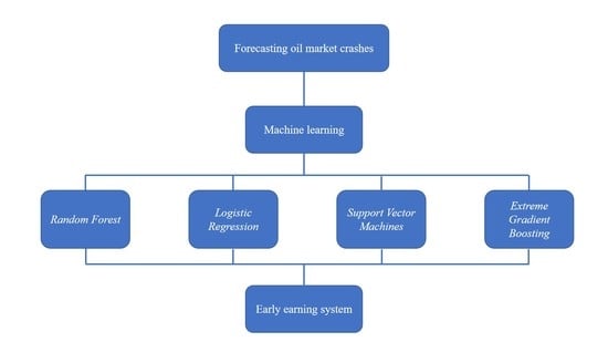
We define the crisis based on [3,15]. Our investigation contributes to the current literature by analyzing the predictive performance of a series of state-of-the-art statistical machine learning methods, including random forest, logistic regression, support vector machine, and extreme gradient boosting (XGBoost) algorithms, in the classification problem of crude oil futures price market crash detection in America, covering the period from 1990 to 2019. To the best of our knowledge, this study provides new insights into forecasting oil price crashes, employing a moving window that has never been reported in the past. Furthermore, we also consider the previous data in the moving window algorithm, and the experimental work presented here provides a novel result that discarding previous data can achieve better performance. We develop an exhaustive experimental performance evaluation of our algorithms using a test dataset of the daily returns performance of the 25-year oil price market.

Finally, we find that the fixed-length window provides a better result than the expanding window, which indicates that we should occasionally abandon distant historical data, and XGBoost outperforms the other techniques in this study, achieving a detection rate as high as 86% using the fixed-length moving window for Dataset2.

The remainder of this paper is organized as follows. Section 2 reviews the previous literature related to this study. We provide a brief explanation of the machine learning algorithms and the moving window utilized in Section 3. In Section 4, we elaborate on the dataset implemented to perform the system. In Section 5, we present an experimental evaluation and provide empirical results. We evaluate the empirical findings based on a series of assessments, computed on a test dataset sample spanning a long period. Finally, we present some concluding remarks in Section 6.

2. Literature Review

The topic of oil price forecasting has been extensively studied [6,7,8]. High- and low-inventory variables have been used to forecast short-run crude oil prices [16]. The results show that global non-oil industrial commodity prices are the most successful predictors of oil prices [6]. Moshiri and Foroutan [17] developed a nonlinear model to forecast crude oil futures prices.

With the development of machine learning and deep learning, an increasing number of academic studies have attempted to research this problem using a machine learning algorithm [9,10,11,12,13]. Wen et al. [9] make crude oil price forecasting based on support vector machines. An empirical model decomposition based neural network ensemble learning paradigm is proposed for oil spot price forecasting [10]. An improved oil price forecast model that uses a support vector machine was developed [18]. Some researchers forecast the crude oil price using machine learning [12] and the deep learning ensemble approach [14]. Other researchers use XGBoost [13] and wavelet decomposition and neural network model [11] to forecast crude oil prices. However, compared with the specific figures of crude oil prices, investors and practitioners are more concerned about the drops or crashes of crude oil prices.

An analytic network process model is applied in forecasting the crisis [19]. There are many papers on predicting financial crises [3,15,20] that apply machine learning. Lean et al. [20] employ the general regression neural networks to predict the currency crisis upon the disastrous 1997–1998 currency crisis experience. Based on a multinomial logit model, Bussiere and Fratzscher [15] develop a new EWS model to forecast financial crises. Chatzis et al. [3] use deep and statistical machine learning techniques (classification trees, support vector machines, random forests, neural networks, extreme gradient boosting, and deep neural networks) to predict stock market crisis events. They find that forecasting accuracy can be improved by adding oil variables to the traditional predictors of excess stock returns of the S&P 500 index. However, investigations into oil price crashes are still very inadequate. The experimental work presented here provides one of the first investigations into how to forecast crashes of crude oil future prices using machine learning.

Chatzis et al. [3] detect a crisis event based on the number of stock market negative coexceedances (less than 1% percentile of the empirical distribution). Due to the imbalanced dataset, and because we want to obtain more crash events, we consider crash events in less than 2.5% percentile of the empirical distribution [15].

A new EWS model for predicting financial crises was developed based on a multinomial logit model in [15], and the model correctly predicts the majority of crises in emerging markets. The 2008 financial crisis brought huge losses to the financial industry, as well as society as a whole, and people gained renewed awareness of the importance of an EWS. Davis and Karim [21] assess and suggest that the logit is the most beneficial approach to a global EWS, along with signal extraction for country-specific EWS for banking crises on a comprehensive common dataset. Babecky et al. [22] account for model uncertainty using Bayesian model averaging, identifying early warning indicators of crises specific to developed economies. The study indicates that the dynamic Bayesian network models can offer precise early-warnings compared with the logit and signal-extraction methods [23].

Studies on EWSs for financial crises employing machine learning techniques are still limited. This paper develops an EWS that includes artificial neural networks, decision trees, and a logistic regression model [24]. Geng et al. [25] use data mining techniques to build financial distress warning models and find that the performance of neural networks is better than decision trees, support vector machines, and multiple classifiers. Finally, a total of six deep and statistical machine learning techniques are used to develop the EWS and forecast a stock market crisis [3].

In this paper, we performed the forecasting model using random forests (hereafter RF) [26], logistical regression (hereafter LogR) [27], support vector machines (hereafter SVMs) [28], and extreme gradient boosting (hereafter XGBoost). RF is applied in gene expression analysis [29], protein–protein interactions [30], risk assessment [31], and image classification [32], among others. Ohlson [27] uses LogR for the first time to predict corporate bankruptcy based on financial statement data. LogR and NN (neural networks) are employed to predict the bond rating [33]. SVMs are widely used in credit rating systems in many investigations [34,35]. XGBoost is an important and efficient implementation of the gradient boosting framework in the classification methodology of [36,37].

In terms of oil price crashes forecasting, there are many methods that can be employed. It includes nearest neighbors [38], NN (neural network), which is broadly applied in credit rating classification [39,40], and LSTM (long short-term memory), it is employed in forecasting the volatility of stock price index [41]. In the future, in addition to adding other methods, we can also consider improve the existing approach. Zhong and Enke [42] use the nature dimensionality reduction technique, means principal component analysis (PCA), and the artificial neural networks (ANNs), yielding improved outcomes.

3. Model Development

We utilized the following models: RF [26], LogR [27], SVMs [28], and XGBoost. Then, we presented a detailed interpretation of the development and parameter tuning of each machine learning methodological framework.

We used the machine learning models above, and we also considered two patterns of moving window corresponding to Section 4, aimed to investigate if there is any difference when historical data are discarded. One is the fixed-length window and the other is the expanding window.

In terms of the fixed-length window, for daily data, we considered 1000 days (almost five years) as the window length, and the first training data was the dataset of the first 1000 records starting from the first day (covering the period 18 June 1990 to 28 September 1994). We considered the 1001st piece of data as the first piece of daily test data. For every subsequent piece of test data (one day in the examined period), we incorporated a new record as the training data, and to keep the window length fixed, we rejected the first observation at the same time. Additionally, for the last observation of daily data in the sample (i.e., 18 December 2019), the empirical distribution of returns ended with the period 23 October 2015 to 17 December 2019. As the daily dataset had 7146 data points, we could obtain 6146 results of test data daily.

As for the expanding window, for daily data, we considered the first 1000 records as the first training data to test the 1001st observation (the first piece of test data), such as the fixed-length window. However, for each subsequent observation (one day in the examined period), the difference is, we incorporated a new observation again as the new training data (and did not discard the first observation). As the total return records was 7146 daily pieces of data, we considered the window length to increase from 1000 to 7145. Additionally, for the last observation of daily data in the sample (i.e., 18 December 2019), the empirical distribution of returns was based on the period from 18 May 1990 to 17 December 2019. We could also obtain 6146 results of test data daily.

3.1. Random Forest (RF)

RF is a combination of tree predictors, where every tree depends on the value of a random vector sampled independently with the same distribution for all trees in the forest [26]. This is a well-known machine learning technique and is applied in gene expression analysis [29], protein–protein interactions [30], risk assessment [31], and image classification [32], financial bankruptcy forecasting [43], among others. In order to implement the RF technique, there is a common package in R named randomForest, which is provided by Liaw and Wiener [44]. We tried using this package to forecast crashes as, because of the huge size of the dataset, the speed of calculation was very slow. Liaw and Wiener [45] also show that the randomForest package is not a fast implementation for high-dimensional data. A fast implementation of random forests for high-dimensional data, called rangers, was introduced. We employed the ranger package in R here [46].

The specific process of this algorithm is as follows. Here is a dataset D that consists of many features denoted by $X_1-X_N$, and the dependent variable $Y$. The dependent variable here is binary, so we could develop a classification problem. As one of the hyperparameters, num.trees (here called n), we considered n as the number of decision trees that RF is expected to generate, and the group was called the Forest. The other hyperparameter mtry (here called m), which means the number of variables to possibly split at each node, and m < N. We tuned the hyperparameter using the tuneRF function, which has the aim of searching for the optimal value of m for RF. We set a specific value for n and the optimal value for m, and by testing several n values based on the model assessment, we could obtain a relatively good result for m and n. Based on this, we also tried to perform some numerical modification. We implemented the algorithm on the basis of the modification in R.

3.2. Logistic Regression (LogR)

LogR is a famous statistical approach using logistic regression to perform classification, which is usually used in differentiating binary dependent variables. Babecky et al. [22] use LogR for the first time to predict corporate bankruptcy based on financial statement data. LogR and NN (neural networks) are employed to predict the bond rating [33]. A credit scorecard system is also usually built [47]. We develop the LogR in R via the glm function, which is used to fit generalized linear models, specified by giving a symbolic account for the linear predictor and an account for the error distribution. We adjust the thresholds due to the imbalance between the crash and no crash events.

3.3. Support Vector Machines (SVMs)

SVMs [28,48] are learning machines for two group classification problems. SVMs are widely used in credit rating systems in many investigations [34,35]. In this study, we tested the SVMs using linear, radial basis function (RBF), polynomial, and sigmoid kernels. In order to choose the proper kernel, we changed the kernel by using it into the moving window and, finally, selected the polynomial kernel. We considered soft-margin SVMs. For the cost hyperparameters, C, of the SVMs (relative to the soft-margin SVMs), and the $I3$ hyperparameter, we employed a grid-search algorithm. We also considered the different weights of crash event and no crash event according to the proportion of the imbalanced dataset. We implemented this SVMs algorithm in R using the e1071 package, along with the grid-search functionality, in this package.

3.4. Extreme Gradient Boosting (XGBoost)

The last main approach we used in this study to predict the crude oil market turbulence is the XGBoost (extreme gradient boosting) algorithm. It is an important and efficient implementation of the gradient boosting framework in the classification methodology of [36,37]. Two algorithms are included: one is the linear model and the other is the tree-learning algorithm. It also provides multifarious objective functions, which include classification, regression, and ranking. We developed XGBoost in this study by using the XGBoost R package. Here, we employed a tree-learning model to perform a binary classification.

We selected the statistical machine learning techniques after taking the general performance and the calculation time required. In addition to the above methods, there are many other approaches that can be applied in this field. It includes the nearest neighbors [38], NN (neural network), and LSTM (long short-term memory). Especially, NN is a famous machine learning algorithm and it is broadly employed in credit rating classification filed [39,40]. A simple NN model is composed of three types of layers, which includes the input layer, hidden layer, and output payer. In the input layer, there are the all candidate variables as a high dimensional vector, and the it is transformed into a lower-dimensional potential information in the hidden layer, and then the output layer can generate the predictions by using the non-linear functions, such as a sigmoid. Even we could also consider using SGD (stochastic gradient descent), PCA (principal component analysis), and the neural network Adam to optimal the model in the future.

Following the moving window that corresponds to Section 3.2, we tested the series of entailed hyperparameters, including the maximum depth of the generated trees, the maximum number of central processing unit threads available, and the maximum number of iterations (for classification, it is similar to the number of trees to grow). On account of the nature of the dependent variable, we employed the “binary: logistic” objective function to train the model. For a better understanding of the learning process, we used an evaluation metric of the area under the receiver operating characteristic (AUROC) to obtain a value for the area under the curve (AUC). The AUROC curve is a performance measure for classification problems at various threshold settings, and the AUC shows the capability of distinguishing between classes. In the analysis, the value of AUC usually varies between 0.5 and 1, and a higher AUC value demonstrated that the model could better distinguish the crash and no crash events. An AUC value of above 0.9 (the result of the last prediction in the moving window) indicates a very good performance of the algorithm in this study.

4. Data Collection and Processing

We considered various relative variables to forecast crashes in the crude oil markets. On the other hand, we also considered whether the variables could provide an adequate data sample. Based on the criteria, we excluded those variables with a relatively short time series. We used the futures prices of crude oil from 13 June 1986 to 18 December 2019, and the futures prices of natural gas and gold, as well as the futures prices of agricultural commodities, which included rough rice, wheat, corn, sugar, cocoa, and canola. We also considered data from the VIX index, the S&P 500 stock price index, and the yield of the USA 10-year bond from 8 June 1990 to 18 December 2019 for daily data. The data were sourced from Bloomberg and Datastream, and detailed information can be seen in

Table 1. Exploratory variables in the model.

Variable	Data	Data Source
Crude Oil	WTI Crude Oil futures prices	Bloomberg
Natural Gas	Henry Hub Natural Gas futures prices
VIX Index	Chicago Board Options Exchange Volatility Index
Bond	USA 10-year bond yield
Stock	S&P 500
Gold	Gold futures prices
Rough Rice	Rough Rice futures prices
Wheat	Wheat futures prices	Datastream
Corn	Corn futures prices
Sugar	Sugar futures prices	Bloomberg
Cocoa	Cocoa futures prices
Canola	Canola futures prices

Note: WTI is the West Texas intermediate. VIX is the Volatility Index.

.

As a result, we obtained a 30-year period for daily data, which included many crude oil futures price crashes. In this way, we filled the datasets with 7146 records for daily use. They provide the capability for modeling contagion dynamics, financial markets, and commodity market interdependencies over time.

In [3], the crisis event is detected based on an empirical distribution that is less than the 1% percentile. In order to obtain more crash event samples, we defined the crash event as less than the 2.5% percentile of the empirical distribution due to the imbalanced dataset, following [15]. That is, we defined the “crash event” ($Cras{h}_{OI{L}_t}$) at each working day. If the log return (hereafter return) of the crude oil futures prices is less than the 2.5% percentile of the empirical distribution of the return, it can be detected. We could obtain a binary variable of the crude oil futures price crashes as follows:

$$Cras{h}_{OI{L}_t}=\{\begin{array}{lll}1 \mathrm{if} R_{OI{L}_t}& <E(R_{OI{L}_t}|I_{OI{L}_{t-1}})& -2\sqrt{Var(R_{OI{L}_t}|I_{OI{L}_{t-1}})}\\ 0& \mathrm{otherwise}& \end{array},$$

(1)

where $R_{OI{L}_t}$ is the log return of crude oil futures prices, $I_{OI{L}_{t-1}}=\{R_{OI{L}_{t-1}},R_{OI{L}_{t-2}}\cdots \}$ is the information set, $E(R_{OI{L}_t}|I_{OI{L}_{t-1}})$ denotes the sample mean of time t under condition $I_{OI{L}_{t-1}}$, and $\sqrt{Var(R_{OI{L}_t}|I_{OI{L}_{t-1}})}$ is the standard deviation of the crude oil futures prices of time t under condition $I_{OI{L}_{t-1}}$.

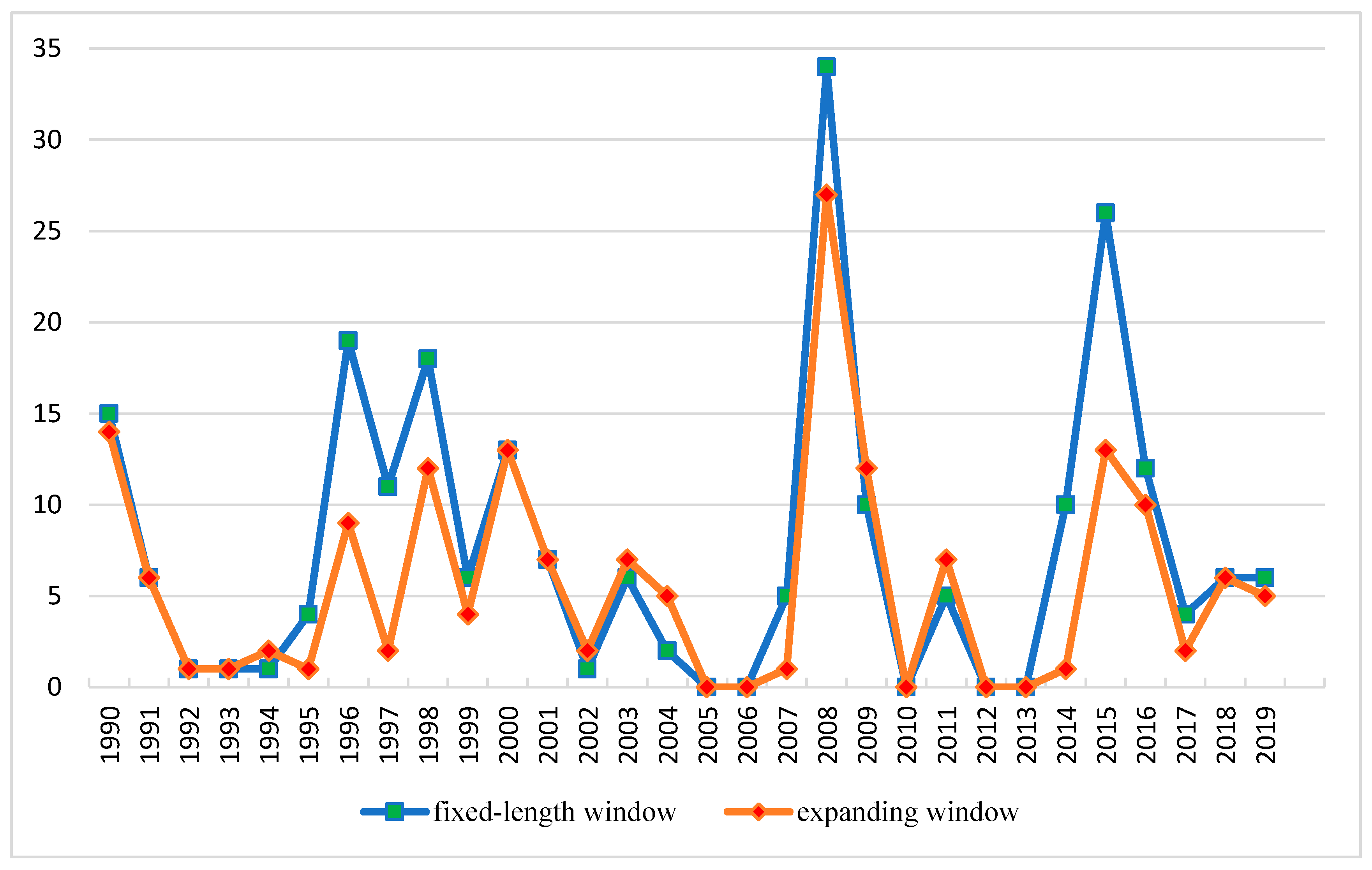
Based on this, we employed two patterns of moving window to calculate the crash events. One is the fixed-length window and the other is the expanding window.

In terms of the fixed-length window, for daily data, we considered 1000 days (almost five years) as the window length and calculated the initial empirical distribution of returns (starting from the first day) based on the crude oil futures prices returns of the first 1000 observations (covering the period from 16 June 1986 to 7 June 1990). We could detect if the 1001st is a crash event according the first empirical distribution of daily returns. For each subsequent data point (day in the examined period), we recalculated the empirical distribution of returns and incorporated a new record, and in order to keep the window length fixed, we rejected the first observation at the same time. The crash event can be identified when the return was below the 2.5% percentile of the new empirical distribution. In addition, for the last observation of daily data in the sample (i.e., 18 December 2019), the empirical distribution of returns ended with the period 23 October 2015 to 17 December 2019.

For the expanding window, for daily data, we could calculate the first empirical distribution based on the first 1000 records to identify the 1001st observation, similar to the fixed-length window. However, for each subsequent observation (day in the examined period), the difference is that we calculated the empirical distribution of returns and incorporated another new observation (we did not discard the first observation). As the total daily return records total 8152, we considered the window length to increase from 1000 to 8151. In addition, for the last observation of daily data in the sample (i.e., 18 December 2019), the empirical distribution of returns was based on the period of 16 June 1986 to 17 December 2019.

Ultimately, we obtained 7152 daily crash records (binary variables). We created the extended variables to take Lag1 to Lag5 of return (we elaborated these in

Table 2. Extended variables. Returns are the log returns.

Variable	Transformation
rash (binary variables)	Lag1–Lag5, L5D
IX Index	Lag1–Lag5
Crude Oil futures prices	Lag1–Lag5, Lag1–Lag5 of returns
Natural Gas futures prices
USA 10-year bond yield
S&P 500
Gold futures prices
Rough Rice futures prices
Wheat futures prices
Corn futures prices
Sugar futures prices
Cocoa futures prices
Canola futures prices

Note: L5D is the average of the crash events for the last five working days.

), so we omitted the first six crash records.

Figure 1 shows the number of crude oil market crashes for daily data during the selected 30-year period. We could see several severe crashes in the daily and weekly frequencies, especially in 1990, 1996, 2008, and 2015. The most severe crashes were in the global crisis of 2008, and the number of crashes was up to 35.

On the other hand, the raw data used are shown in Table 1. In order to get the most out of the raw data and give full play to the machine learning models, we extended the raw variables and obtain the extended variables. To predict the crash events, we considered the previous data of crash events as a fairly predictive indicator, so we also considered the binary variables of crash events.

We made the following transformations based on the exploratory variables to capture the subtler dependencies and dynamics. Detailed information is displayed in Table 2.

• We computed the lagged variables on a daily basis for each crash indicator, starting from one to five days (Lag1–Lag 5).
• Except for the Crash variable (binary variables) and VIX index (because it is a volatility index, we did not return to it), we took the return of the other variables. Then, using (i), we calculated the lagged variables of the return variables again.
• We calculated the average number of crash events for the last five working days (L5D), according to the binary variables of crash events on a daily basis.

We also developed two predictive indicator datasets to see how much the performance of the machine learning models improves. One had only the Crash (Lag1–Lag5) and the crude oil futures prices (Lag1–Lag 5, Lag1–Lag5 of returns) and the average of crash events for the last five working days (L5D; hereafter Dataset1), and the other had all predictive indicators (hereafter Dataset2). In Dataset1, there were 16 predictors, and in Dataset2, there were 121 predictors. For daily data, the dataset had 7146 data points, spanning from 18 June 1990 to 18 December 2019.

5. Experimental Evaluation

After we obtained the confusion matrix of the various models for machine learning, we performed an experimental evaluation procedure. In other words, we showed the performance results for the evaluation of the models covering a long period (1994–2019 for daily data), which included several crash events.

5.1. Model Validation Measures

Classification accuracy is the main criterion for evaluating the efficiency of each approach and for selecting the most robust method according to discriminatory power. We provided several metrics that are widely used to quantitatively assess the discriminatory power of each machine learning model. However, our dataset faced an issue of imbalanced amounts of the two classes, called imbalanced data. For example, in terms of the fixed length of the moving window for daily data, there were 6146 data points in total, in which only 205 were “CRASH.” Even if we obtained high classification accuracy, we could not consider the model to perform well. As such, there is a risk that the assessment norm we used may misinterpret based on the skewed class distribution. For the imbalanced data, we wanted to know the capacity of predicting the minority of the dataset.

Bekkar et al. [49] presented a set of evaluation measures for model assessment over imbalanced datasets. First, they obtained the sensitivity and specificity based on the confusion matrix and considered combined measures (G-means, likelihood ratios, F-measure balanced accuracy, discriminant power, the Youden index, and the Matthews correlation coefficient). They also considered the graphical performance assessment (receiver operating characteristic (ROC) curve, area under curve, etc.). Due to the application of the moving window, we could not obtain the AUC value based on the area under the curve metrics, so we do not consider the AUC as the general metric. In a similar way, we do not use the graphical performance assessment. In machine learning, the two classes of forecasting method are assessed by the confusion matrix, such as in

Table 3. Confusion matrix for two-class classification.

	Predicted No Crash	Predicted Crash
Actual no crash	TN	FP
Actual crash	FN	TP

Note: TP = True Positive, means the number of positive cases (i.e., crash) that are identified as positive correctly; FP = False Positive, shows the number of negative vases (i.e., no crash) that are misclassified as positive cases; FN = False Negative, indicates the number of positive cases that are incorrectly identified as negative cases; TN = True Negative, is the number of negative cases that are correctly identified as negative cases.

. The raw data represents the real value of the class label, while the column represents the classifier prediction. In the imbalanced dataset, the observations of the minority class were defined as positive, and the observations of the majority were labeled negative. Here, positive means “CRASH,” negative means “NO CRASH.” Following [38], we adopted the sensitivity and specificity metrics, which are defined as follows.

Using the confusion matrix given by Table 3, we could calculate the sensitivity and specificity as follows:

$$Sensitivity=\frac{TP}{TP+FN}$$

(2)

$$Specificity=\frac{TN}{TN+FP}$$

(3)

Sensitivity is the ratio of true positive to the sum of true positive and false negative, i.e., the proportion of actual positives that are correctly identified as such. Specificity is the ratio of true negative to the sum of true negative and false positive, i.e., the proportion of actual negatives that are correctly identified as such. Based on sensitivity and specificity, we calculated several combined evaluation measures as follows:

G-mean: The geometric mean (G-mean) is the product of sensitivity (accuracy on the positive examples) and specificity (accuracy on the negative examples). The metric indicates the balance between classification performances in the minority and majority classes. The G-mean is defined as follows:

$$G=\sqrt{Sensitivity\times Specificity}$$

(4)

Based on this metric, even though the negative observations are correctly classified per the model, a poor performance in the prediction of the positive examples will lead to a low G-mean value.

LR (+): The positive likelihood ratio (LR (+)) represents the ratio between the probability of predicting an example as positive when it is truly positive and the probability of the predicted example being positive when, in fact, it is not positive. We have

$$LR (+)=\frac{Sensitivity}{1-Specificity}$$

(5)

LR (−): The negative likelihood ratio (LR (−)) is defined as the ratio between the probability of predicting an example as negative when it is actually positive, and the probability of predicting an example as negative when it is truly negative. It is written as:

$$LR (-)=\frac{1-Sensitivity}{Specificity}$$

(6)

As we can see, the higher LR (+) and lower LR (−) show better performance in the positive and negative classes, respectively.

DP: Discriminant power (DP) is a metric that summarizes sensitivity and specificity, defined as follows:

$$DP=\frac{\sqrt{3}}{\pi }\left(log\frac{Sensitivity}{1-Sencitivity}+log\frac{Specificity}{1-Specificity}\right)$$

(7)

A DP value higher than 3 indicates that the algorithm distinguishes between positive and negative examples.

BA: The balanced accuracy (BA) assessment is the average of sensitivity and specificity. This metric performs equally well in either class. It holds:

$$BA=\frac{1}{2}\left(Sensitivity+Specificity\right)$$

(8)

In contrast, if the conventional accuracy is high only because the classifier can distinguish the majority class (i.e., ‘no crash’ in our study), the BA value will drop.

WBA: The weighted balanced accuracy (WBA) is the weighted average of sensitivity of 75% and a specificity of 25% on the basis of BA [3].

Youden index: The Youden index$\gamma$ measures the ability of the algorithm to avoid failure. It is defined as:

$$\gamma =Sensitivity+Specificity-1$$

(9)

Generally, a higher value of $\gamma$ indicates a better ability to avoid misclassification.

We used these criteria to perform a comprehensive measurement of the discriminative power of each technique. On the basis of these outcomes, we inferred an optimal cutoff threshold of the predicted crash probabilities for each fitted model, pertaining to the optimal sensitivity and specificity metrics. The results of each evaluation are displayed in

Table 4. Model validation measures of daily data for Dataset1.

Window for Fixed-Length	RF	LogR	SVMs	XGBoost
G-mean	0.509	0.806	0.501	0.846
LR (+)	7.852	5.028	3.750	8.339
LR (−)	0.758	0.276	0.786	0.232
DP	0.560	0.695	0.374	0.858
BA	0.617	0.807	0.599	0.848
WBA	0.443	0.786	0.435	0.819
Youden	0.234	0.614	0.199	0.695
Window for Expanding	RF	LogR	SVMs	XGBoost
G-mean	0.345	0.590	0.406	0.463
LR (+)	3.717	1.837	1.699	2.998
LR (−)	0.907	0.716	0.915	0.832
DP	0.338	0.226	0.148	0.307
BA	0.545	0.606	0.538	0.578
WBA	0.334	0.536	0.361	0.405
Youden	0.090	0.212	0.076	0.155

Note: In Dataset1, there are 16 predictors. G-mean represents the geometric mean, LR (+) is the positive likelihood ratio, LR (−) denotes the negative likelihood ratio, DP denotes the discriminant power, BA represents the balanced accuracy, and Youden denotes the Youden index I3.

and

Table 5. Model validation measures of daily data for Dataset2.

Window for Fixed-Length	RF	LogR	SVMs	XGBoost
G-mean	0.459	0.527	0.421	0.847
LR (+)	3.766	3.690	10.116	5.124
LR (−)	0.825	0.760	0.834	0.164
DP	0.364	0.378	0.597	0.824
BA	0.582	0.610	0.581	0.847
WBA	0.403	0.456	0.381	0.855
Youden	0.165	0.220	0.163	0.695
Window for Expanding	RF	LogR	SVMs	XGBoost
G-mean	0.402	0.560	0.296	0.366
LR (+)	3.058	2.102	5.807	5.956
LR (−)	0.878	0.754	0.925	0.883
DP	0.299	0.245	0.440	0.457
BA	0.558	0.601	0.537	0.557
WBA	0.364	0.492	0.313	0.347
Youden	0.115	0.201	0.074	0.114

Note: In Dataset2, there are 121 predictors. G-mean represents the geometric mean, LR (+) is the positive likelihood ratio, LR (−) denotes the negative likelihood ratio, DP denotes the discriminant power, BA represents the balanced accuracy, and Youden denotes the Youden index I3.

. As we could infer from Table 4 and Table 5, both in Dataset1 and Dataset2, in terms of a fixed-length window, XGBoost could lead to the highest classification accuracy, and in the case of an expanding window, LogR outperformed XGBoost.

5.2. Accuracy of the Generated Alarms

In conclusion, we provided a new insight into developing an early warning system for increasing awareness of an impending crash event in the crude oil futures prices market, using machine learning techniques, which included random forest, logistic regression, support vector machine, and extreme gradient boosting algorithms. We calculated an optimal oil futures price crash probability cut-off threshold for each model, and when the predictive probabilities exceed the settled threshold, an alarm will be generated.

As we can see from

Table 6. Classification accuracy table for Dataset1.

Fixed-Length Window
RF	pred		LogR	pred		SVMs	pred		XGBoost	pred
ture	0	1	Ture	0	1	ture	0	1	ture	0	1
0	5738	203	0	5036	905	0	5832	454	0	5378	563
1	150	55	1	48	157	1	175	65	1	43	162
Signal	FAR	DR	Signal	FAR	DR	Signal	FAR	DR	Signal	FAR	DR
Rate	3%	27%	Rate	15%	77%	Rate	7%	27%	Rate	9%	79%
Expanding Window
RF	pred		LogR	pred		SVMs	pred		XGBoost	pred
ture	0	1	Ture	0	1	ture	0	1	ture	0	1
0	5801	199	0	4479	1521	0	5437	653	0	5534	466
1	128	18	1	78	68	1	119	27	1	112	34
Signal	FAR	DR	Signal	FAR	DR	Signal	FAR	DR	Signal	FAR	DR
Rate	3%	12%	Rate	25%	47%	Rate	11%	18%	Rate	8%	23%

Note: In Dataset1, there are 16 predictors. FAR represents false alarm rate, $\mathrm{FAR}=\frac{FP}{FP+TN}$; DR represents detection rate, and DR = $\frac{TP}{TP+FN}$.

and

Table 7. Classification accuracy table for Dataset2.

Fixed-Length Window
RF	pred		LogR	pred		SVMs	pred		XGBoost	Pred
ture	0	1	ture	0	1	ture	0	1	ture	0	1
0	5587	354	0	5454	487	0	5835	106	0	4940	1001
1	159	46	1	143	62	1	168	37	1	28	177
Signal	FAR	DR	Signal	FAR	DR	Signal	FAR	DR	Signal	FAR	DR
Rate	6%	22%	Rate	8%	30%	Rate	2%	18%	Rate	17%	86%
Expanding Window
RF	pred		LogR	pred		SVMs	pred		XGBoost	Pred
ture	0	1	ture	0	1	ture	0	1	ture	0	1
0	5664	336	0	4905	1095	0	5908	92	0	5862	138
1	121	25	1	90	56	1	133	13	1	126	20
Signal	FAR	DR	Signal	FAR	DR	Signal	FAR	DR	Signal	FAR	DR
Rate	6%	17%	Rate	18%	38%	Rate	2%	9%	Rate	2%	14%

Note: In Dataset2, there were 121 predictors. FAR represents false alarm rate, FAR = $\frac{FP}{FP+TN}$; DR represents detection rate, and DR = $\frac{TP}{TP+FN}$.

, we obtained the final confusion matrix for all the evaluated models. The results of the false alarm rate and detection rate are also shown. Concentrating on the best-performing model, namely the XGBoost of the fixed-length window, by accepting a 9% false alarm rate, we succeeded in forecasting 79% of futures price crashes in the crude oil market for Dataset1. Under a false alarm rate of 17%, we could even predict 86% of crashes for Dataset2.

6. Some Concluding Remarks

Financial crisis prediction plays a pivotal role for both practitioners and policymakers, as they can infer crashes and recessions through an early warning system, being able to perform relevant actions that curtail the contagion crisis or preempt an economic crisis or recession.

Firstly, we chose the most significant financial market indicators to help forecasting and perform changes that capture the subtler dependencies and dynamics, and defined the crash event as less than the 2.5% percentile of the empirical distribution. Then we selected the statistical machine learning techniques after taking the general performance and the calculation time required, and we developed the evaluated models by tuning the hyperparameter and obtained the optimal performance of each algorithm. We employed the evaluation metrics that are broadly used to assess the discriminatory power of a binary classifier on imbalanced datasets, finally.

Lean et al. [20] developed a general regression neural network (GRNN) currency forecasting model, and compared its performance with those of other forecasting methods. An early warning system was also developed using artificial neural networks (ANN), decision trees, and logistic regression models to predict whether a crisis happens within the upcoming 12-month period [24]. Additionally, the result shows ANN has given superior results. Chatzis et al. [3] use a series of techniques including classification trees, SVMs, RF, NN, XGBoost, and deep neural networks to forecast the stock market crisis events, and find that deep neural networks built using the MXNET library is the best forecasting approach. Our investigation concerns developing machine learning models that can be continuously retrained in moving window setup, which Chatzis et al. [3] do not challenge. Next, many previous investigations only use accuracy to measure the predictive ability of machine learning methods [20,24]. However, in terms of the imbalanced dataset, we were concerned about whether the crisis or crash event can be predicted precisely, rather than the no crisis or no crash event. Additionally, we regarded the detection rate as important.

The main novel contribution of this empirical investigation to the existing literature is that it fills the gap of futures prices forecasting in the crude oil market, and we pioneered the use of a moving window in this field. We also made a comparison where the previous data were discarded.

Our empirical results show the following:

• Except for the LogR for Dataset2, in other machine learning algorithms, the fixed-length window shows a better performance than the expanding window. This indicates that discarding historical data is a better choice in forecasting the future.
• XGBoost outperformed the rest of the employed approaches. It could even reach an 86% detection rate using the fixed-length moving window for Dataset2.
• The performances of Dataset1 and Dataset2 did not differ significantly, meaning the indicators that are only about crude oil futures prices and crashes were very important.

These findings made our study much more attractive to researchers and practitioners working in petroleum-related agencies. The result of XGBoost also provided strong evidence that it could offer a good starting point for developing an early warning system.

For future work, first, we will consider feature engineering and perform feature selection to improve the accuracy of Dataset2. Chatzis et al. [3] show that deep neural networks significantly increase classification accuracy for forecasting stock market crisis events. Owing to the use of the moving window, we encountered some difficulties in coding when we wanted to implement the neural network technique. We will work hard to overcome this in future work.