Review

Towards the Correct Measurement of Thermal Conductivity of Ionic Melts and Nanofluids †

by
Carlos A. Nieto de Castro
* and
Maria José V. Lourenço
Centro de Química Estrutural, Faculdade de Ciências, Universidade de Lisboa, Campo Grande, 1749-016 Lisbon, Portugal
*
Author to whom correspondence should be addressed.
Presented at the 1st International Conference on Nanofluids, Castelló, Spain, 26–28 June 2019.
Energies 2020, 13(1), 99; https://doi.org/10.3390/en13010099
Submission received: 19 November 2019 / Revised: 13 December 2019 / Accepted: 19 December 2019 / Published: 24 December 2019

Abstract

:
Thermophysical properties of engineering fluids have proven in the past to be essential for the design of physical and chemical processing and reaction equipment in the chemical, metallurgical, and allied industries, as they influence directly the design parameters and performance of plant units in the of, for example, heat exchangers, distillation columns, phase separation, and reactors. In the energy field, the search for the optimization of existing and alternative fuels, either using neutral or ionic fluids, is an actual research and application topic, both for new applications and the sustainable development of old technologies. One of the most important drawbacks in the industrial use of thermophysical property data is the common discrepancies in available data, measured with different methods, different samples, and questionable quality assessment. Measuring accurately the thermal conductivity of fluids has been a very successful task since the late 1970s due to the efforts of several schools in Europe, Japan, and the United States. However, the application of the most accurate techniques to several systems with technological importance, like ionic liquids, nanofluids, and molten salts, has not been made in the last ten years in a correct fashion, generating highly inaccurate data, which do not reflect the real physical situation. It is the purpose of this paper to review critically the best available techniques for the measurement of thermal conductivity of fluids, with special emphasis on transient methods and their application to ionic liquids, nanofluids, and molten salts.

Graphical Abstract

1. Introduction

Thermal conductivity has been proven to be one of the most difficult properties of materials to be measured with high accuracy. This fact is due to the different molecular mechanisms of heat transfer in solids, liquids, and gases, with neutral or ionic media, and to the difficulties involved in the isolation of pure conduction from other mechanisms of heat transfer, like convection and radiation, a fact that arises from the contradictory requirements of imposing a temperature gradient on the fluid while preventing its motion. This is particularly important in steady state measurements, where the temperature in any point of the measured sample is time independent, and where the heat flux necessary to keep a temperature difference between two surfaces is measured. For isotropic fluids, the thermal conductivity is defined by the Fourier’s law, depends on the thermodynamic state of the fluid prior to the perturbation, and must be related with a reference state, not necessarily equal to the initial one [1].
q = λ T
where q is the instantaneous flux of heat, the response of the medium to the instantaneous temperature gradient T , and λ the thermal conductivity of the medium. As it is impossible to measure local fluxes and local gradients, the Fourier equation cannot be used directly, and the energy equation must be adapted to a given geometry. The equation of energy conservation in the system is the basis for the formulation of the working equation of any method of measurement of thermal conductivity. The equation of change for non-isothermal systems can be found on the excellent book by Bird, Stuart, and Lightfoot [2], which is written for unit mass as:
ρ D U D t = ( · q ) P ( · v ) ( τ : v )
where ρ is the fluid density, U its internal energy, t the time, P the hydrostatic pressure, v the hydrodynamic velocity of the fluid, and τ the stress tensor. This equation does not include nuclear, radiative, electromagnetic, or chemical terms for energy. In addition, it is applicable to Newtonian fluids; otherwise the last term of Equation (2) must be reformulated for viscoelastic fluids. The notation D/Dt represents the substantial derivative, meaning that the time rate of change is reported as one move with the fluid (The substantial derivative is given by D D t = t + v · ). From a point of view of experiment, the temperature time evolution is more convenient to obtain. After some manipulation, using the definition of enthalpy and heat capacity at constant pressure, C P , we can obtain the equation of change for temperature:
ρ C P D T D t = ( · q ) ( τ : v ) ( ln ρ ln T ) P
If the sample is not moving (solid of stationary fluid, no convection), the properties of the sample do not vary with temperature (small temperature gradients), and using the Fourier law (Equation (1)), this last equation cane be transformed to:
ρ C P T t = 2 T
where 2 is the symbol for the Laplacian operator. It is important to recognize that transport of energy by radiation is always present, and must be corrected for each measuring technique, especially if measurements are performed at high temperatures. Then, terms corresponding to the radiative energy absorption and emission rates must be added. Equation (4) is the basis of all experimental methods for the measurement of thermal conductivity.
Between 1950 and 1990, a variety of experimental methods have been developed, for gaseous, liquid, supercritical or solid phases, over wide range of thermodynamic states. Until the 1970s much of the experimental work on the thermophysical properties of fluids was devoted to the development of methods for the measurement of the properties of simple fluids under moderate conditions. By the end of the 1970s a few methods emerged that had both a rigorous mathematical description of the experimental method and technical innovation to render measurements precise enough to rigorously test theories of fluids for both gas and liquid phases. It was also possible with the development of electronics and fast data acquisition systems, to establish highly accurate instrumentation and methods for fluids (gases and liquids) and solids for wide temperature and pressure ranges and the establishment of standard reference data. The reader can obtain a lot of information in references [3,4,5,6].
These methods are based on the simplified energy equation and can be classified in two main categories:
-
Unsteady state or transient methods, in which the full Equation (4) is used and the principal measurement is the temporal history of the fluid temperature (transient hot-wire, transient hot strip, the interferometric technique adapted to states near the critical point etc.);
-
Steady state techniques, for which T t = 0 and the equation reduces to 2 T = 0 , which can be integrated for a given geometry (parallel plates, concentric cylinders, etc.).
However, it is difficult and tedious to make good measurements of thermophysical properties. Nowadays it is also neither fashionable nor economically attractive for industries and funding agencies, and the need for accurate data on the thermophysical properties of fluids has been replaced to a certain extent by alternative methods of properties calculation, mostly based on computer simulation or prediction/estimation methodologies (cheaper, but risky), and by the apparent contradiction between accurate (low uncertainty) or fit for purpose. This last approach supported the development of many commercial types of equipment, which were developed with the main objective of being user friendly and fast.
Reasons for this can be summarized in the following items:
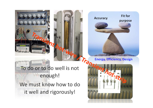
  • Change of needs—From laboratory work to in-situ measurements,
  • Change of paradigm—Fit for purpose instead of best uncertainty,
  • Change of financing priorities from state funding agencies—priority to industry driven/sponsored research,
  • Decrease for users in industry of the added value of property data of good quality,
  • The use and misuse of commercial equipment’s, with methods of measurement not adequate to the object systems.
Current practice shows that, despite being based on established methods, construction, and type of fluid/solid to be applied to, several inaccuracies exist in the data obtained and sometimes to completely erroneous results. This is the case of their application in the fluids area to new and more complex systems like humid air, nanofluids, ionic melts (molten salts and ionic liquids) and nanofluids.
Figure 1 shows the situation for the thermal conductivity of molten alkali nitrates in 2016. Data was selected accordingly to our selection of “best data”. Details of the authorship and references can be found in the paper by Nunes et al., 2016 [7]. It shows important scattering of data between different authors for de same salt/mixture, much greater than the claimed mutual uncertainty of data. An extraordinary example is the data presented in Janz NIST database (1979) [8] and the paper by Nagasaka et al., 1991 for potassium nitrate (KNO3), where positive or negative slopes can be observed [9].
It is the purpose of this paper to review critically the best available techniques for the measurement of thermal conductivity of fluids, with special emphasis on transient methods and their application to ionic liquids, nanofluids, and molten salts. In addition, several remarks on how theory can help to access the quality of data obtained.

2. Methods of Measuring Thermal Conductivity of Ionic Melts and Nanofluids

It is not the purpose of this paper to describe in detail all the methods developed so far for the measurement of the thermal conductivity, namely for the temperature range 300–1500 K, at ambient pressure, the main zone where ionic liquids, molten salts and nanofluids are important and have several industrial applications. Several of these methods can be applied also to lower temperature melts/systems, and to solids. A complete discussion of the situation can be seen in the paper by Mardolcar and Nieto de Castro, 1992 [5]. From classical methods (transient hot-wire, concentric cylinders or parallel plates) to non-classical methods (laser flash, forced Rayleigh scattering, photon correlation spectroscopy, photothermal radiometry, transient thermoreflectance, photothermal detection, wave-front-shearing interferometry, heat flow, AC calorimetry, photoacoustic and radiation heat exchange), all are there described, instrumentally and mathematical modelling of the different physical situations, identifying all the advantages and disadvantages of each method. To these, we must add the transient hot strip method, the transient plane source or hot-disk and the 3ω method, all developed after 1992.
The methods are classified as primary and secondary, as explained in the reference [10] (The definition of primary method was approved by CCQM—Comité Consultatif pour la Quantité de Matière, BIPM, in 1995—“a primary method of measurement is a method having the highest metrological qualities, the operation of which can be completely described and understood, for which a complete uncertainty statement can be written down in terms of SI units, the results of which are therefore accepted without reference to a standard of the quantity being measured.”). The values quoted for the attainable uncertainty correspond to the “state-of-art” of the method and cannot be compared with commercial instruments, which as mentioned above, sacrifice high accuracy for ease of operation and cost of equipment. Transient methods are the only ones that can compete for the statute of primary methods, in the sense of CIPM2. These methods include the transient hot-wire and the transient hot strip, the latter still requiring the solution of 3D heat transfer equation for the geometries involved.
Table 1 displays selected methods for the measurement of thermal conductivity (thermal diffusivity) and its applicability to ionic melts and nanofluids, after a careful selection by the authors of the most likely to have success in the measurements. This methodology was applied before by the authors in two different papers, one dedicated to low temperature ionic liquids and molten salts [10], and more recently to nanofluids [11], and it is improved here for comparison. Reference must also be made to four methods for the determination of thermal diffusivity, α = λ ρ C P , which are not direct measurements of thermal conductivity, needing accurate values of density (usually available) and heat capacity (more difficult to obtain), the laser flash [12,13], the photon-correlation spectroscopy [14], the forced Rayleigh scattering method [15], and the transient grating technique [16]. The first one has potential for high temperature melts and nanofluids, the second one is a very versatile an amenable to improvement method, the third one has been applied to molten salts and the fourth one contains the first reported measurements for the thermal conductivity of LTILs. Some discussion of the methods applicable to nanofluids can be found in the work of Bobbo and Fidele [17].
From all these methods, only the transient hot-wire can be today considered as a primary method. In fact [18]:
-
The transient hot wire technique was identified as the best technique for obtaining standard reference data (certification of reference materials).
-
It is an absolute technique, with a working equation and a complete set of corrections reflecting the departure from the ideal model, where the principal variables are measured with a high degree of accuracy. It is accepted by the scientific community as a primary method, the top of the traceability chain for this physical quantity.
-
The liquids proposed by IUPAC (toluene, benzene, and water) as primary standards for the measurement of thermal conductivity were measured with this technique with an accuracy of 1% or better.
-
It has been extended, from its original version, to its application at high temperatures (correction for radiation effects), for conducting liquids and melts.
Although several texts in the past have described the complete theory of the method and its application to gases and liquids, we would like to make a short description because many commercial applications, although mentioning that their method is based on the hot-wire principles, do not pay attention to many deviations from the ideal mathematical model.
The theory of the transient hot wire is well known, and a complete uncertainty analysis has been previously presented [19,20,21]. The ideal mathematical model of an infinite vertical line heat source immersed in an infinite isotropic medium with properties independent of the temperature, and in thermodynamic equilibrium T0 at t = 0, and when a stepwise heat flux q per unit length is applied to the wire, generates a pure conductive heat flux that will transfer from the wire to the immersed medium, obtained from the solution of Equation (4), that will increase as a function of time the temperature at the surface of the wire, decaying in the media, as a function of time and distance to the centre of the wire, r. This temperature rise can be defined as:
Δ T ( r , t ) = T ( r , t ) T 0
Equation (4) can be solved subjected to boundary conditions:
Δ T ( r , t ) = 0 for   t 0 , any   r lim r 0 Δ T ( r , t ) = 0 for   t > 0 lim r 0 r T r = q 2 π λ = constant   for   t 0
where the additional condition that the thermal diffusivity α = λ ϱ C P is constant [22]. The result for the ideal temperature rise is:
Δ T id ( r , t ) = T ( r , t ) T 0 = q 4 π λ E 1 ( r 2 4 α t )
where E1(x) is the exponential integral. This integral can be expanded by:
E 1 ( r 2 4 α t ) = r 2 4 α t 0 e y y d y =   γ ln ( r 2 4 α t ) + r 2 4 α t + O [ ( r 2 4 α t ) 2 ]
where γ = 0.5772157 … being the Euler’s constant. If the line source is replaced by a cylindrical wire of radius ri (as small as possible) and assuming that the temperature of the fluid in the ideal model is equal to the temperature at the surface of this wire, at r = ri. Then, for small values of r 2 4 α t , we can obtain:
Δ T id ( r i , t ) = T ( r i , t ) T 0 = q 4 π λ ln ( 4 α t r i 2 C ) + r i 2 4 α t +
where C = exp (γ). The radius must be as small as possible and therefore if the term r i 2 4 α t < 0.01 % of Δ T id , then the temperature increases at the surface of the hot-wire is given by:
Δ T id ( r i , t ) = T ( r i , t ) T 0 = q 4 π λ ln ( 4 α t r i 2 C )
Equation (10) is the fundamental working equation of the transient-hot wire technique, if the conditions used for its derivation are realized experimentally. If so, the thermal conductivity can be obtained from the slope of the straight line Δ T id versus logarithm of time and referred to the temperature T ( r i , t ) , if measured experimentally.
However, the real model of the transient hot wire constructed in any instrument has departures from the ideal mathematical model, namely the finite diameter of the wire, its finite physical properties, its finite length, and its supports. Using the transient hot wire method, the uncertainty of the experimental determined thermal conductivity derives from uncertainty associated to other modes of heat transfer such as convection and radiation, and from the uncertainty associated with random and systematic errors in the measurement of input quantities [20]. Consequently, the experimental measurements of the temperature rise of the wire, Δ T w , depart from the ideal temperature rise Δ T id predicted by Equation (10) and a set of small corrections δ T i must be added to the actual temperature rise, given by:
Δ T id ( r i , t ) = Δ T w ( r i , t ) + i δ T i
Most of these corrections were devised by Healy et al. [23]. Some effects can be minimized by proper design of the instrument, but others must be accounted for. The various corrections δ T i are summarized elsewhere [19,24], the contribution to the global uncertainty of the thermal conductivity of these corrections never amount to more than 0.1% of thermal conductivity [21], when a proper design is made. However, Healy et al. [23] also noted that the thermal conductivity must be assigned, not to T0 but to a reference thermodynamic state (Tref, ρref) defined as:
T ref =   T 0 + i δ T i * ϱ ref = ϱ ( T ref   ,   P 0 )
These corrections δ T i * are essentially two. δ T 1 * refers to the fact that the bulk fluid properties are temperature dependent. This fact causes one correction, that is time dependent and is better used in the correction to the temperature rise ( δ T 7 ) and another part, constant in time, δ T 1 * given by:
δ T 1 * = 1 2   [ Δ T ( t i ) + Δ T ( t f ) ]
Here ti and tf are the initial and final times of the measurement interval used in the regression line. The second correction δ T 2 * is to be utilized if the metal wire is coated, with a metal oxide or a polymer to insulate electrically the wire from an electrically conducting media (like an ionic liquid, an electrolyte solution or a molten salt), and expressions were proposed in first place by Nagasaka and Nagashima in 1981 [25]. In this case, the value of Δ T ( t 2 ) in Equation (13) must be calculated at the surface of the coat [25]. A systematic analysis of the departures us presented in references [19,24], and here in Table 2 with the necessary adaptations.
Several comments must be made. Some of the corrections have to be applied to have accurate measurements ( δ T 1 ,   δ T 2 ,   δ T 5 ,   δ T 7 ,   δ T 8 ,   δ T 10 ,   δ T 1 * ,   δ T 2 * ), and some others must be rendered negligible by a careful instrument design ( δ T 3 ,   δ T 6 ,   δ T 9 ). Once this approach is made, it is possible to obtain straight lines with very good statistics, like those shown in Figure 2. This data was obtained with an instrument specially developed in Lisbon for corrosive environments, humid air, with an expanded uncertainty (k = 2) of 1.7%. The hot-wire cells are presented in Figure 3 and details of it can be find in reference [35].
A more recent, alternative approach to the approximate analytic solution described above is to solve the full Fourier heat transfer equations in the wire and the test material, using numerical methods based upon the finite element method (FEM). This procedure was developed and validated with water by Antoniadis et al. [36], using a two-tantalum hot wires system. Agreement between the two procedures was within 0.2% at 297.5 K and atmospheric pressure. Both the FEM method and the approximate analytic solution herein described have uncertainties of 0.5%. Applications to nanofluids of TiO2 and MWCNTs showed that, when the measurements are judiciously performed, with a validated “state of art” instrument, the results can even prove which earlier results were correct.
A final comment deserves attention, as many measurements are made with mixtures. In fact, the imposition of a temperature gradient in the fluid mixture generates a diffusive molecular/ionic flux, driven by one or more chemical potential/composition gradients, namely thermal diffusion or the Soret Effect. If in steady-state methods it can be assumed that it becomes zero and the Fourier Law defined the thermal conductivity, in transient methods, this is not obvious [19]. For a mixture of perfect gases, the same happens for the transient hot-wire method, and no mass transfer exists at the surface of the wire. Thus, we can assume that this result is kept for dense gases and liquids, and there no change in the working equation. Accordingly, Equations (10)–(13) can be applied to mixtures.
In principle, the hot-wire method can be applied to ionic melts and nanofluids, if a careful design is made of the instrument. However, the reliability and accuracy of instruments used to measure thermal conductivity of ionic melts has to consider several problems, which can influence the accuracy of the data obtained. Starting with the ionic melts, we have:
-
High temperature measurements (molten salts).
-
Radiation must be corrected or minimized, and convection eliminated.
-
Electrical insulation of measuring probes indispensable.
-
Use of current commercial instrumentation, such as transient hot-probes and transient hot-strips/disks, based on adaptations of the heat source immersed in the fluid exact behaviour, sacrifice accuracy at the cost of instrumentation and ease of handling of probes and samples. The accountability of methods must be proven.
-
Many of the results presented in the bibliography were taken with commercial instrumentation, and not properly validated.
-
In the limited context of hot wire, for instance, it is common to use just one wire, sometimes shorter than the model requires (end effects), which directly affects the accuracy of the measurements.
For the case of nanofluids, we can consider in addition that thermal conductivity is the property most influenced by the nanoparticles present. For a current analysis of the problem, see the recently published work of Antoniadis et al. [36]. In addition [11], the nanofluids can be electrically conducting (water, metal particles, nanocarbons, etc.) and when the ordinary transient hot-wire is applied to measure the thermal conductivity of electrical conducting liquids, several problems are encountered, as explained above, but can be summarized here:
-
The contact between the bare metallic wire and the conducting liquid provides a secondary path for the flow of current in the cell and the heat generation in the wire cannot be defined unambiguously.
-
Polarization of the liquid occurs at the surface of the wire, producing an electrical double-layer.
-
The electrical measuring system (an automatic Wheatstone bridge) that detects the changes in the voltage signals in the wire is affected by the combined resistance /capacitance effect, caused by the dual path conduction.
-
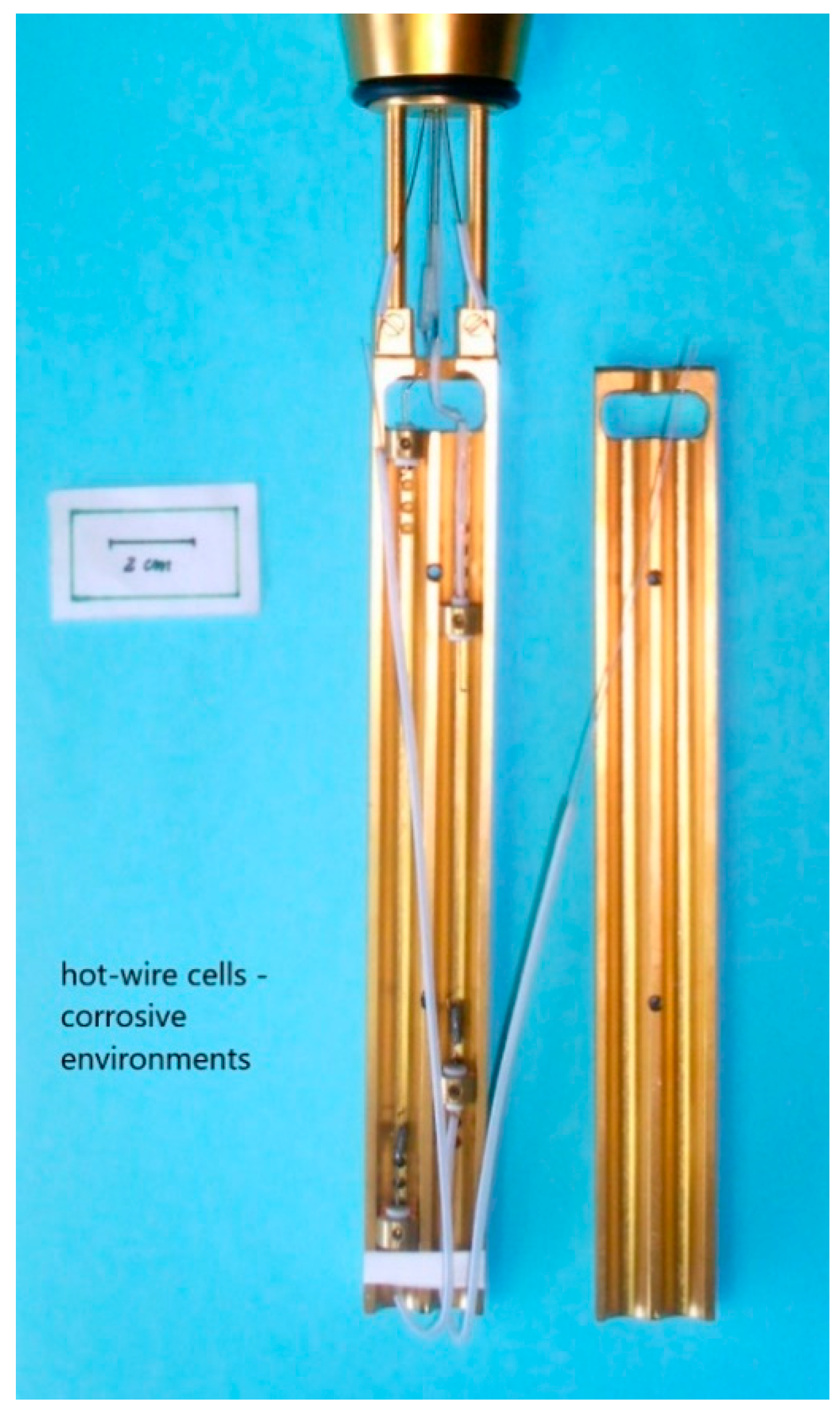
Insulated wires (necessity to cover the wire with materials or insulating anodizing coatings to protect it during the measurements) or polarized techniques are required [11].
Secondly, the generation of a high temperature gradient near the wire might create migration of nanoparticles to its surface and deposition of particles in the surface of the probes, creating nanostructures with organization dependent of surface of the probe/hot-wire, that vary the thermal conductivity of the non-perturbed nanofluid, giving rise to anomalous measured effects. It also changes its bulk concentration, distorting the propagation of the heating wave, making the sensing zone non-homogeneous, and originating a temperature discontinuity like the temperature jump in gases. A hot wire-nanofluid interface thermal conductance (sometimes referred to as the Kapitza resistance) needs to be measured, and this fact can be detected experimentally, as explained by Rutin and Skripov, 2017 [37] and Hasselman, 2018 [38]. Recent work in ionanofluids of graphene and carbon nanotubes in our group, using molecular simulation, showed that not only this interphase exists, but also that it has a finite value of thermal conductivity, of the order of 15–30% that of the bulk ionic liquid [39].
This is magnified when the nanoparticles have surface charges that create a problem equivalent to ions. This will affect the modelling of the measurement and will create erroneous results. These problems are not considered by instrument manufacturers, and especial probes must be designed on purpose. Tertsinidou et al. [40] have developed a comprehensive study of several nanofluids (ethylene glycol with added CuO, TiO2, or Al2O3 nanoparticles and water with TiO2 or Al2O3 nanoparticles or MWCNTs) and proved that the transient-hot wire method and the hot disk thermal analyser can produce comparable accurate results within 2% mutual uncertainty, if measurements are performed accordingly to the recommendations above. Their transient hot-wire cells are displayed in Figure 4. Figure 5 shows the results obtained compared with other authors.
In high temperature applications, like molten carbonates (T > 600 K) [49], the use of hot-wire geometries is limited, as very robust sensors are required. Geometries based on thin hot-wires cannot be used, due to their fragility. High temperature melts are solids at room temperature, have high surface tensions in the liquid phase, are strongly active, and both chemically and electrically conductive. Molten materials attack most materials either by chemical corrosion or physical erosion depending on the various environments, hence changing their chemical and physical properties. No known singular material satisfies all requirements and operation at high temperatures is always associated with some degree of interaction with the environment. So, any measuring probe must protect the sensing element from chemical or physical attacks, and therefore materials compatibility is a very challenging problem.
Until now, there have been no accurate experimental results with molten salts at very high temperatures. However, efforts to develop hot-strip sensors for high temperature in situ chemical gas streams have opened the way to their applications to molten salts and nanosalts (nanofluids of molten salts) [50].
Ceramic/thin metal film-based sensors, were designed, constructed, and applied for thermal conductivity measuring sensors, inspired in previous works of the group, by Lourenço et al. [51,52]. Platinum resistance thermometers were also developed using the same technology, to be used in the temperature measurement, were also constructed, and tested, using Al2O3 protecting electrically insulating coatings. The data acquisition system uses a linearization of the transient hot-strip model [53,54]. The model shows that the temperature rise at the surface of the hot strip is linearly proportional to the logarithm of a dimensionless time, τ, as displayed in Equations (14)–(16).
τ = 2 a f t w a f = λ ρ C P
Δ T s = T ( t ) T 0 = q s 2 λ π f ( τ )
f ( τ ) = τ erf ( 1 τ ) τ 2 4 π [ 1 exp ( 1 τ 2 ) ] + 1 4 π E 1 ( 1 τ 2 )
where af is the thermal diffusivity of the media, qs is the heat dissipated per unit length of the strip, w is the width of the strip, τ, is a dimensionless time, and λ, ρ, τ,, and CP are, respectively, the thermal conductivity, density, and heat capacity at constant pressure of the media. The mathematical functions erf (y) and E1 (z) are, respectively, the error function and the exponential integral, obtainable from rational approximations and easily programmed. Figure 6 shows one of the sensors.
The dynamic response for a run with the sensor immersed in air can be seen in Figure 7, expressed as the temperature rise in the hot strip as a function of ln τ , with the optimal operating zone in red.
The equipment can measure the thermal conductivity of gaseous phases with an accuracy of 2–5% up to 840 °C, (95% confidence level). The extension of the sensors operating zone up to 1200 °C is under way, as are their assessment in high temperature melts.

3. Conclusions

The measurement of the thermal conductivity of ionic melts and nanofluids is proposed to be done with accurate methods of measurement, in order to have confidence in the quality of the results. The transient hot wire continues to be the best available technique to obtain good data, although methods like the transient hot strip, laser flash, hot disk, and photo-correlation spectroscopy (transparent fluids) might be a less accurate but cheaper method. Most equipment manufacturers sacrifice accuracy to easiness and speed of operation, and in most cases, produce bad data, which cannot be validated with standard reference data or certified reference materials. The art of measuring in thermal sciences is a continuously challenging field, especially when new and more complex systems for new applications appear. It is not enough to measure it, but rather to measure it well, and with an uncertainty compatible with the expected future use of the data.

Author Contributions

All the authors contributed equally to all manuscript. All authors have read and agreed to the published version of the manuscript.

Funding

This work was partially funded by FCT—Fundação para a Ciência e para a Tecnologia, Portugal, through Centro de Química Estrutural (UID/QUI/0100/2019).

Acknowledgments

This article is based upon work from COST Action Nanouptake, supported by COST (European Cooperation in Science and Technology) www.cost.eu. The authors would like to thank the members of this Action for several fruitful discussions along the years of 2017-19. The authors would also like to thank all the collaborators and partners in the field of thermal conductivity measurements, namely, J.M.N.A. Fareleira, U.V. Mardolcar, M.L.V. Ramires, A. Gurova, H.M. Roder, R.A. Perkins, M.J. Assael and, specially, to Sir W.A. Wakeham, who taught CANC the Art of Measuring Thermal Conductivity and the Tricks of the Trade.

Conflicts of Interest

The authors declare no conflict of interest.

References

  1. Nieto de Castro, C.A. Absolute measurements of the viscosity and thermal conductivity of fluids. JSME Int. J. Ser. II 1988, 31, 387–401. [Google Scholar] [CrossRef] [Green Version]
  2. Bird, R.B.; Stewart, W.E.; Lightfoot, E.N. Transport Phenomena, 2nd ed.; John and Wiley and Sons, Inc.: New York, NY, USA, 2002. [Google Scholar]
  3. Wakeham, W.A.; Nagashima, A.; Sengers, J.V. Measurement of the Transport Properties of Fluids: Experimental Thermodynamics; Blackwell Scientific Pubs: Oxford, UK, 1991; Volume III. [Google Scholar]
  4. Nieto de Castro, C.A.; Li, S.F.Y.; Nagashima, A.; Trengove, R.D.; Wakeham, W.A. Standard reference data for the thermal conductivity of liquids. J. Phys. Chem. Ref. Data 1986, 15, 1073. [Google Scholar] [CrossRef] [Green Version]
  5. Mardolcar, U.V.; Nieto de Castro, C.A. The measurement of thermal conductivity at high temperatures. High Temp. High Press. 1992, 24, 551. [Google Scholar]
  6. Assael, M.J.; Goodwin, A.R.H.; Vesovic, V.; Wakeham, W.A. Experimental Thermodynamics Volume IX: Advances in Transport Properties of Fluids; Especially Chapter 5; Royal Society of Chemistry: London, UK, 2014. [Google Scholar]
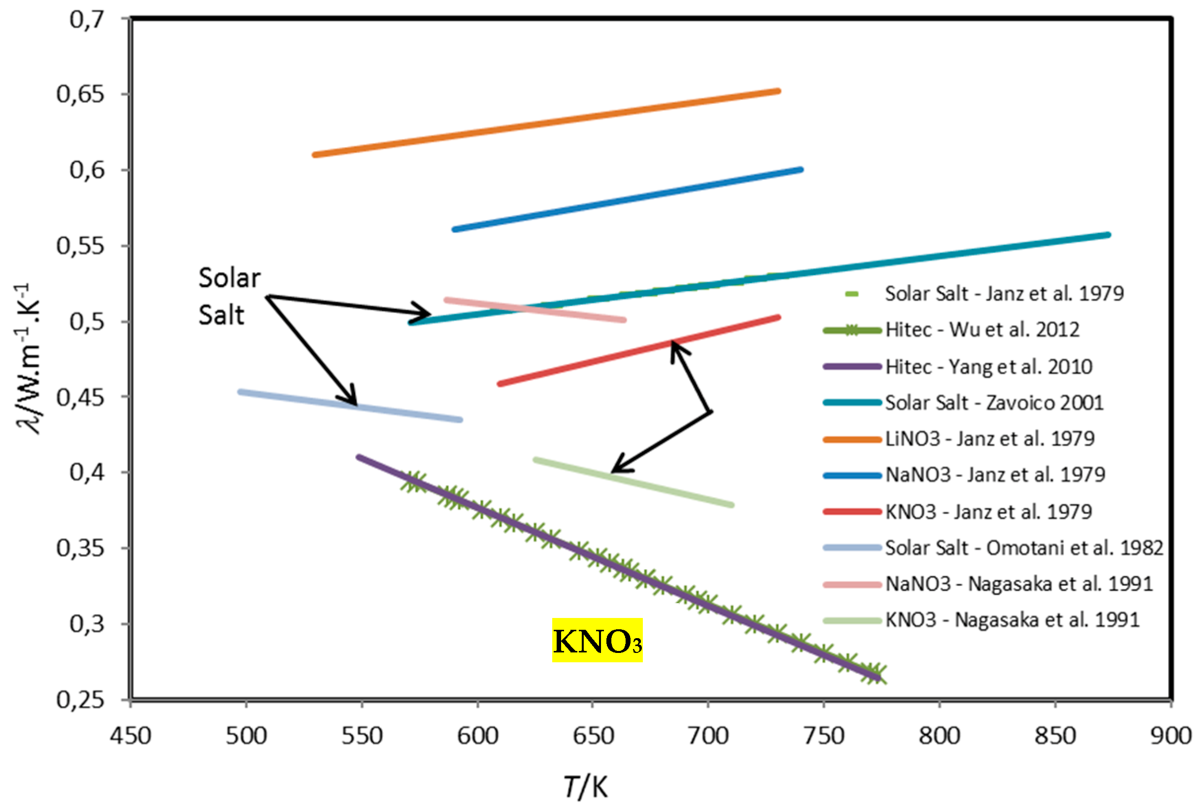
  7. Nunes, V.M.B.; Queirós, C.S.; Lourenço, M.J.V.; Santos, F.J.V.; Nieto de Castro, C.A. Molten salts as engineering fluids—A review: Part I. Molten alkali nitrates. Appl. Energy 2016, 183, 603–611. [Google Scholar] [CrossRef]
  8. Janz, G.J.; Allen, C.B.; Bansal, N.P.; Murphy, R.M.; Tomkins, R.P.T. Physical Properties Data Compilations Relevant to Energy Storage; NSRDS-NBS 61; Part II; USA Department of Commerce: Washington, DC, USA, 1979.
  9. Nagasaka, Y.; Nagashima, A. The Thermal Conductivity of Molten NaNO3 and KNO3. Int. J. Thermophys. 1991, 12, 769–781. [Google Scholar] [CrossRef]
  10. Nunes, V.M.B.; Lourenço, M.J.V.; Santos, F.J.V.; Matos Lopes, M.L.S.; Nieto de Castro, C.A. Accurate Measurement of Physico-Chemical Properties on Ionic Liquids and Molten Salts. In Ionic Liquids and Molten Salts: Never the Twain; Seddon, K.E., Gaune-Escard, M., Eds.; John Wiley & Sons, Inc.: New York, NY, USA, 2010; pp. 229–263. [Google Scholar]
  11. Nieto de Castro, C.A.; Vieira, S.I.C.; Lourenço, M.J.V.; Sohel Murshed, S.M. Understanding Stability, Measurements, and Mechanisms of Thermal Conductivity of Nanofluids. J. Nanofluids 2017, 6, 804–811. [Google Scholar] [CrossRef]
  12. Tada, Y.; Harada, M.; Tanigaki, M.; Egushi, W. Laser flash method for measuring thermal conductivity of liquids-Application to low thermal conductivity liquids. Rev. Sci. Instrum. 1978, 49, 1305–1314. [Google Scholar] [CrossRef]
  13. Lee, S.W.; Park, S.D.; Kang, S.; Shin, S.H.; Kim, J.H.; Bang, I.C. Feasibility study on molten gallium with suspended nanoparticles for nuclear coolant. Nucl. Eng. Des. 2012, 247, 147–159. [Google Scholar] [CrossRef]
  14. Kraft, K.; Lopes, M.M.; Leipertz, A. Thermal-diffusivity and thermal-conductivity of toluene by photon-correlation spectroscopy—A test of the accuracy of the method. Int. J. Thermophys. 1995, 16, 423–432. [Google Scholar] [CrossRef]
  15. Nagasaka, Y.; Nakazawa, N.; Nagashima, A. Experimental determination of the thermal conductivity of molten alkali halides by the forced Rayleigh scattering method. I. Molten LiCl, NaCl, KCl, RbCl and CsCl. Int. J. Thermophys. 1992, 13, 555–574. [Google Scholar] [CrossRef]
  16. Frez, C.; Diebold, G.J.; Tran, C.D.; Yu, S. Determination of the thermal diffusivities, thermal conductivities, and sound speeds of room-temperature ionic liquids by the transient grating technique. J. Chem. Eng. Data 2006, 51, 1250–1255. [Google Scholar] [CrossRef]
  17. Bobbo, S.; Fidele, L. Experimental methods for the characterization of thermophysical properties of nanofluids. In Heat Transfer Enhancement with Nanofluids; Bianco, V., Manca, O., Nardini, S., Vafai, K., Eds.; CRC Press: Boca Raton, FL, USA, 2015; Chapter 4. [Google Scholar]
  18. Nieto de Castro, C.A. State of Art in Liquid Thermal Conductivity Standards. In Proceedings of the Invited Communication to BIPM-CCT-WG9 Meeting, Bratislava, Slovak Republic, 9 September 2005. [Google Scholar]
  19. Assael, M.J.; Nieto de Castro, C.A.; Roder, H.M.; Wakeham, W.A. Experimental Chemical Thermodynamics. In Measurement of the Transport Properties of Fluids; Wakeham, W.A., Nagashima, A., Sengers, J.V., Eds.; Blackwells: Oxford, UK, 1991; Volume 2, Chapter 7. [Google Scholar]
  20. Ramires, M.L.V.; Nieto de Castro, C.A. Uncertainty and Performance of the Transient Hot Wire Method. In Proceedings of the Tempmeko 2001, 8th International Symposium on Temperature and Thermal Measurements in Industry and Science, Berlin, Germany, 19–21 June 2002; Fellmuth, B., Seidel, J., Scholz, G., Eds.; Vde Verlag GmbH: Berlin, Germany, 2002; Volume 2, pp. 1181–1886. [Google Scholar]
  21. Beirão, S.G.S.; Ramires, M.L.V.; Dix, M.; Nieto de Castro, C.A. A New Instrument for the Measurement of Thermal Conductivity of Fluids. Int. J. Thermophys. 2006, 27, 1018–1041. [Google Scholar] [CrossRef]
  22. Carslaw, H.S.; Jaeger, J.C. Conduction of Heat in Solids; Oxford University Press: London, UK, 1959; p. 256. [Google Scholar]
  23. Healy, J.; de Groot, J.J.; Kestin, J. The Theory of the Transient Hot-wire Method for Measuring Thermal Conductivity. Physica 1976, 82, 392–408. [Google Scholar] [CrossRef]
  24. Nieto de Castro, C.A.; Taxis, B.; Roder, H.M.; Wakeham, W.A. Thermal Diffusivity Measurement by the Transient Hot-Wire Technique: A Reappraisal. Int. J. Thermophys. 1988, 9, 293–316. [Google Scholar] [CrossRef]
  25. Nagasaka, Y.; Nagashima, A. Absolute Measurement of the Thermal Conductivity of Electrically Conducting Liquids by The Transient Hot-Wire Method. J. Phys. E Sci. Instrum. 1981, 14, 1435–1440. [Google Scholar] [CrossRef]
  26. Fisher, J. Zur Bestimmung der Wärmeleitfähigkeit und der Temperaturleitfähigkeit aus dem Ausgleichvorgang beim Schleiermacherschen Meßrohrverfahren und beim Plattenverfahren. Ann. Phys. 1939, 34, 669–688. [Google Scholar] [CrossRef]
  27. Nieto de Castro, C.A. Medida da Condutibilidade Térmica de Hidrocarbonetos Líquidos pelo Método do Fio Aquecido. Ph.D. Thesis, Instituto Superior Técnico, UTL, Portugal, 1977. [Google Scholar]
  28. Goldstein, R.J.; Briggs, D.G. Transient Free Convection about Vertical Plates and Circular Cylinders. J. Heat Trans. 1964, 86, 490–500. [Google Scholar] [CrossRef]
  29. De Groot, S.R.; Kestin, J.; Sookiazian, H. Instrument to measure the thermal conductivity of gases. Physica 1974, 75, 454–482. [Google Scholar] [CrossRef]
  30. Nagasaka, Y.; Nagashima, A. Simultaneous measurement of the thermal conductivity and thermal diffusivity of fluids. High Temp. High Press. 1989, 21, 363–371. [Google Scholar]
  31. Menashe, J.; Wakeham, W.A.; Bunsenges, B. The Thermal Conductivity of n-Nonane and n-Undecane at Pressures up to 500 MPa in the Temperature Range 35–90 °C. Phys. Chem. 1981, 85, 340–347. [Google Scholar] [CrossRef]
  32. Nieto de Castro, C.A.; Li, S.F.Y.; Maitland, G.C.; Wakeham, W.A. Thermal Conductivity of Toluene in the Temperature Range 35–90 °C at Pressures up to 600 MPa. Int. J. Thermophys. 1983, 4, 311–327. [Google Scholar] [CrossRef]
  33. Calado, J.C.G.; Fareleira, J.M.N.A.; Nieto de Castro, C.A.; Wakeham, W.A. Reference state in thermal conductivity measurements. Revista Virtual de Química 1984, 26, 173–176. [Google Scholar]
  34. Ramires, M.L.V.; Nieto de Castro, C.A.; Fareleira, J.M.N.A.; Wakeham, W.A. The Thermal Conductivity of Aqueous Sodium Chloride Solutions. J. Chem. Eng. Data 1994, 39, 186–190. [Google Scholar] [CrossRef]
  35. Beirão, S.G.S.; Ribeiro, A.P.C.; Lourenço, M.J.V.; Santos, F.J.V.; Nieto de Castro, C.A. Thermal Conductivity of Humid Air. Int. J. Thermophys. 2012, 33, 1686–1703. [Google Scholar] [CrossRef]
  36. Antoniadis, K.D.; Tertsinidou, G.J.; Assael, M.J.; Wakeham, W.A. Necessary Conditions for Accurate, Transient Hot-Wire Measurements of the Apparent Thermal Conductivity of Nanofluids are Seldom Satisfied. Int. J. Thermophys. 2016, 37, 78. [Google Scholar] [CrossRef]
  37. Rutin, S.B.; Skripov, P.V. Comments on “The Apparent Thermal Conductivity of Liquids Containing Solid Particles of Nanometer Dimensions: A Critique” (Int. J. Thermophys. 2015, 36, 1367). Int. J. Thermophys. 2016, 37, 102. [Google Scholar] [CrossRef]
  38. Haselman, D.P.H. Can the Temperature Dependence of the Heat Transfer Coefficient of the Wire—Nanofluid Interface Explain the “Anomalous” Thermal Conductivity of Nanofluids Measured by the Hot-Wire Method? Int. J. Thermophys. 2018, 39, 109. [Google Scholar] [CrossRef]
  39. França, J.M.P.; Nieto de Castro, C.A.; Pádua, A.A.H. Molecular Interactions and Thermal Transport in Ionic Liquids with Carbon Nanomaterials. Phys. Chem. Chem. Phys. 2017, 19, 17075–17087. [Google Scholar] [CrossRef]
  40. Tertsinidou, G.J.; Tsolakidou, C.M.; Pantzali, M.; Marc, J.; Assael Colla, L.; Fedele, L.; Bobbo, S.; Wakeham, W.A. New Measurements of the Apparent Thermal Conductivity of Nanofluids and Investigation of Their Heat Transfer Capabilities. J. Chem. Eng. Data 2017, 62, 491–507. [Google Scholar] [CrossRef] [Green Version]
  41. Fedele, L.; Colla, L.; Bobbo, S. Viscosity and thermal conductivity measurements of water-based nanofluids containing titanium oxide nanoparticles. Int. J. Refrig. 2012, 35, 1359–1366. [Google Scholar] [CrossRef]
  42. Zhang, X.; Gu, H.; Fujii, M. Experimental Study on the Effective Thermal Conductivity and Thermal Diffusivity of Nanofluids. Int. J. Thermophys. 2006, 27, 569–580. [Google Scholar] [CrossRef]
  43. Duangthongsuk, W.; Wongwises, S. Measurement of temperature-dependent thermal conductivity and viscosity of TiO2—Water nanofluids. Exp. Therm. Fluid Sci. 2009, 33, 706–714. [Google Scholar] [CrossRef]
  44. Yoo, D.H.; Hong, K.S.; Yang, H.S. Study of thermal conductivity of nanofluids for the application of heat transfer fluids. Thermochim. Acta 2007, 455, 66–69. [Google Scholar] [CrossRef]
  45. Reddy, M.C.S.; Rao, V.V. Experimental studies on thermal conductivity of blends of ethylene glycol-water-based TiO2 nanofluids. Int. Commun. Heat Mass Transf. 2013, 46, 31–36. [Google Scholar] [CrossRef]
  46. Yiamsawasd, T.; Dalkilic, A.S.; Wongwises, S. Measurement of the thermal conductivity of titania and alumina nanofluids. Thermochim. Acta 2012, 545, 48–56. [Google Scholar] [CrossRef]
  47. Haghighi, E.B.; Saleemi, M.; Nikkam, N.; Khodabandeh, R.; Toprak, M.S.; Muhammed, M.; Palm, B. Accurate basis of comparison for convective heat transfer in nanofluids. Int. Commun. Heat Mass Transf. 2014, 52, 1–7. [Google Scholar] [CrossRef]
  48. Hamilton, R.L.; Crosser, O.K. Thermal conductivity of heterogeneous two-component systems. Ind. Eng. Chem. Fundam. 1962, 1, 187–191. [Google Scholar] [CrossRef]
  49. Nunes, V.M.B.; Lourenço, M.J.V.; Santos, F.J.V.; Nieto de Castro, C.A. Molten Alkali Carbonates as Alternative Engineering Fluids for High Temperature Applications. Appl. Energy 2019, 242, 1626–1633. [Google Scholar] [CrossRef]
  50. Queirós, C.S.G.P.; Lourenço, M.J.V.; Vieira, S.I.; Serra, J.M.; Nieto de Castro, C.A. New Portable Instrument for the Measurement of Thermal Conductivity in Gas Process Conditions. Rev. Sci. Instrum. 2016, 87, 065105. [Google Scholar] [CrossRef]
  51. Lourenço, M.J.V.; Serra, J.M.; Nunes, M.R.; Vallêra, A.M.; Nieto de Castro, C.A. Thin-Film Characterization for High Temperature Applications. Int. J. Thermophys. 1998, 19, 1253. [Google Scholar] [CrossRef]
  52. Lourenço, M.J.V.; Nieto de Castro, C.A. Measuring the Thermal Conductivity at High Temperatures. Instrumental Difficulties and Sensor Performance. In Proceedings of the Tempmeko 2001, 8th International Symposium on Temperature and Thermal Measurements in Industry and Science, Berlin, Germany, 19–21 June 2002; Fellmuth, B., Seidel, J., Scholz, G., Eds.; Vde Verlag GmbH: Berlin, Germany, 2002; Volume 2, pp. 989–995. [Google Scholar]
  53. Gustafsson, S.E.; Karawacki, E.; Khan, M.N. Transient hot-strip method for simultaneously measuring thermal conductivity and thermal diffusivity of solids and fluids. J. Phys. D Appl. Phys. 1979, 12, 1411–1421. [Google Scholar] [CrossRef]
  54. Gustafsson, S.E.; Karawacki, E.; Khan, M.N. Determination of the thermal-conductivity tensor and the heat capacity of insulating solids with the transientmethod. J. Appl. Phys. 1981, 52, 2596–2600. [Google Scholar] [CrossRef]
Figure 1. Thermal conductivity of molten alkali nitrates and mixtures. Solar salt is a eutectic binary mixture (NaNO3:KNO3 60/40 wt%), while HITEC® is a eutectic ternary mixture (NaNO2: KNO3: NaNO3 7/53/40 wt%). Adapted from [7].
Energies 13 00099 g001
Figure 2. Deviations between the ideal temperature rises and those obtained from the linear regression line—Scattering plot, for a test with humid air, for Tref = 425.92 K, P = 5.00 MPa and yH2O = 0.05097. Adapted from [35].
Energies 13 00099 g002
Figure 3. TiN film protection of TWH instrument for humid air measurements—detail of hot-wire cells. Hot-wire was made from tungsten (diameter 8.94 ± 0.05 µm, long wire length 148.92 ± 0.02 mm and short compensating wire length 71.69 ± 0.02 mm). The global uncertainty of the measurement, at a 95% confidence level, was estimated to be Uλ = 1.7%. Adapted from [35].
Energies 13 00099 g003
Figure 4. Hot-wire cells developed by Antoniadis et al. [36] for the measuring of the thermal conductivity of electrically conducting nanofluids. Tantalum (99.9%) wire (25 µm, long wire length 50 mm and short compensating wire length 20 mm) coated with an anodic layer of Ta2O5. The global uncertainty of the measurement, at a 95% confidence level, was estimated to be Uλ = 1%. Courtesy of the authors.
Energies 13 00099 g004
Figure 5. Thermal conductivity enhancement of water in the presence of TiO2 nanoparticles as a function of the composition for nanoparticles with different diameters [40], at 298.15 K. Bottom-half-solid diamonds, 76 nm, Fedele et al. [41]; Υ, 40 nm, Zhang et al. [42]; ◐, 26 nm, Duangthongsuk and Wongwises [43]; ⌽, 25 nm, Yoo et al. [44]; ◓, 21 nm, Reddy and Rao [45]; ○, 21 nm, Yiamsaward et al. [46]; ◮, 20 nm, Haghighi et al. [47]; , Hamilton–Crosser model [48]; ▲, 30–50 nm (+PVP), THW [40]; △, 5–15 nm (+PVP), THW [40]; triangle with vertical bar, 5 nm, THW [40]; triangle with horizontal bar, 5–15 nm (+PVP), HDTCA [40]. Reprinted with Permission from American Chemical Society (Further permissions related to the material excerpted should be directed to the ACS.).
Energies 13 00099 g005
Figure 6. Transient hot-strip sensor for high temperature thermal conductivity measurement. The sensor is composed by a metallic thin Platinum film, deposited by PVD on an alumina substrate. The hot strip lengths are lL = 15 mm, lS = 5 mm, and thickness w = 110 µm [49].
Energies 13 00099 g006
Figure 7. Dynamic sensor response for a run with the sensor immersed in air, with the optimal operating zone in red [49].
Energies 13 00099 g007
Table 1. Selected methods for the measurement of thermal conductivity (thermal diffusivity) and its applicability to ionic melts and nanofluids.
MethodTypeAttainable Uncertainty 1Applicability to Ionic MeltsApplicability to Nanofluids
YesNoRemarksYesNoRemarks
Transient hot-wire for conducting liquids 2Primary1%The best method to be applied with classical designsThe best method to be applied with classical designs
Transient hot-wire (bare wires)Primary1%Non-conducting base fluids and/or nanoparticles
Transient hot strip for conducting liquids (insulated strip)Primary/Secondary2–3%Can be considered primary if the 3D heat transfer equation is solved for the geometries involvedCan be considered primary if the 3D heat transfer equation is solved for the geometries involved
Transient Plane Source or Hot-DiskSecondary3–5%Limited in temperature rangeLimited in temperature range
Steady-state Parallel Plates (Guarded Hot-Plates)Secondary2–3%Small spacing between plates might induce phase separation
Steady-state Concentric CylindersSecondary2–3%Small gaps. Guarded platesSmall gaps must be used.
Laser FlashSecondary3–5%Difficulties with originated waves in the liquid surface (Marangoni effects)Use low power lasers to avoid NP breakage and structure deployment
Forced Rayleigh ScatteringSecondary/Relative3–5%Dyes necessary to enhance the signal compatible with molten salts or IL’sDyes necessary to enhance the signal compatible with nanofluids.
Photon Correlation SpectroscopySecondary/Relative2–3%Optically transparent fluids. Not explored for measurements above 473 K.Optically transparent fluids.
Transient GratingSecondary/Relative3–5%Needs a big improvement in the calibration. Not recommended for high quality workNeeds a big improvement in the calibration. Not recommended for high quality work
3ω MethodSecondary5%Needs improvement of the theory. However, alternating current, destroying the direction of the polarizing current, avoids current polarizationNeeds improvement of the theory. However, alternating current, destroying the direction of the polarizing current, avoids nanoparticle deposition and electrically insulation problems.
1 Uncertainty is defined using ISO criteria, using a coverage factor (k = 2), that correspond to a 95% confidence level. 2 Both the insulated probe and the polarization technique can be used.
Table 2. Departures from ideal model of transient hot-wire technique.
CorrectionPhysical SourceExpressionReferenceRecommendations
δ T 1 Wire physical properties δ T 1 = q 4 π λ { r i 2 [ ( ρ C P ) w ( ρ C P ) ] 2 λ t ln ( 4 α t r i 2 C ) r i 2 2 α t + r i 2 4 α w t λ 2 λ w } [22,23]Apply always correction.
δ T 2 Outer boundary. Cell physical dimensions (b is cell wall diameter) δ T 2 = q 4 π λ { ln ( 4 α t b 2 C ) + ν = 1 e g ν α t / b 2 [ π Y ( g ν ) ] 2 } [23,26]Apply always correction. Make design of cell to minimize it to 0.1% of Δ T id .
δ T 3 Compression work (L is the wire length and V is the cell volume) δ T 3 = [ q L R t ρ C P C V V ( 1 e b 2 / 4 α t ) + q R 4 C V λ E 1 ( b 2 4 α t ) ] [23,24]Negligible in liquid phases. For gases limits the operational zone of measurements to ρ > 40 kg·m−3.
δ T 4 Radial convection and viscous dissipation. Symbol w means wire properties. (αP is the isobaric thermal expansion coefficient of fluid and g the acceleration of gravity)For gases and liquids (Δρ < ρ0)
δ T 4 = ( q 4 π λ ) 2 α P [ ln 4 + P r g 2 t 2 α P 2 C P ]
For liquids, expressions also graphical form, recording the vertical penetration depth of moving fluid front.
Z p * = Z p λ g α P q t 2 = Z p * ( Pr , t * ,   r * ,   ω )
Pr = η C P λ   ;   t * = α t r i 2 ;   r * = r r i   ;   ω = 2 ρ C P ( ρ C P ) w
[23,24,27,28,29,30]Avoid onset of convection in the measurements. Design measurement time to t < 5 s to render negligible in liquid phases. Wire(s) must be vertical. Avoid short wires.
δ T 5 Radiation (s is the Stefan-Boltzmann constant, K is the a mean extinction coefficient for radiation and n the refractive index of the liquid) Transparent fluid   δ T 5 = 8 π r i σ T 0 3 Δ T i d 2 q
Absorbing fluid
δ T 5 =   q B 4 π λ [ r i 2 4 α ln ( 4 α t r i 2 C ) + r i 2 4 α t ]         w i t h   B 16 K n 2 σ T 0 3 ρ C P
[23,31,32]Always apply correction, dependent if fluid is transparent or absorbs radiation. K is difficult to obtain experimentally, but usually B r i 2 / 4 α <   10 5 [30,32]. Introduces curvature in straight line and it is mostly important at high temperatures (molten salts).
δ T 6 Temperature jump δ T 6 q Λ 2 π λ r i Δ T id T 0 [23,29]Important for gases. Work outside density range where it is not negligible (mean free path of the gas molecules Λ approaching wire diameter (microns). For nanofluids might play a role, but here with nanoparticles dimension.
δ T 7 Effect of variable fluid properties δ T 7 =   [ q 4 π λ ( T 0 ) ] 2 ( χ γ ) ln 4
λ ( T , ρ ) = λ ( T 0 ) ( 1 + χ Δ T )         ρ C P ( T , ρ ) = ρ C P ( T 0 ) ( 1 + γ Δ T )
[24,33]Always apply correction. Valid for situations where fluid density during a measurement can be considered constant, as in the case of systems far from critical region.
δ T 8 Effect of variable fluid properties (fluids critical region) δ T 8 = ( χ γ ) ( q 4 π λ ( T 0 ) ) 3 ln 4 χ 6 Δ T 3
χ = ϕ ρ 0 α P 2 ; r = ε ρ 0 α P 2 ; ε = 1 ρ C P ( T 0 ) [ ( ρ C P ) ρ ] T
[30]Always apply correction. For measurements in the critical region, the properties are extremely strong functions of temperature.
δ T 9 Truncation error resulting from the expansion of exponential integral, Equation (8) δ T 9 =   Δ T i d r i 2 [ 4 α t ln ( 4 α t r i 2 C ) ] [30]Rendered negligible by design. It decreases with time.
δ T 10 Effect of coating to insulate wires for electrically conducting liquids. Subscript 2 means coating properties. r0 is coating radius δ T 9 = B t Δ T i d + q 4 π λ { ln ( r 0 r i ) 2 ( 1 λ λ 2 ) λ 2 λ w 1 t [ D B ln 4 λ r i 2 C ] }
B = 1 2 λ [ r i 2 ( λ 2 α 2 λ w α w ) + r 0 2 ( λ α λ 2 α 2 ) ]
D = r i 2 8 [ ( λ λ 2 λ w ) ( 1 α w + 1 α 2 ) + 4 α 2 2 α w ] + r 0 2 2 ( 1 α + 1 α 2 ) + r i 2 λ 2 ( λ 2 α 2 λ w α w ) ln ( r 0 r i ) + 1 2 λ [ r i 2 ( λ 2 α 2 λ w α w ) + r 0 2 ( λ α λ 2 α 2 ) ] ln 4 α r 0 2 C
[25,34]Always apply correction.
δ T 1 * Effect of variable fluid properties δ T 1 * = 1 2   [ Δ T ( t i ) + Δ T ( t 2 ) ] [4,32,33]Always apply correction. When the distribution of the measured temperature rises is not uniform, a more detailed expression is necessary [32].
δ T 2 * Effect of coating to insulate wires for electrically conducting liquids δ T 2 * = q 8 π λ { 2 ln ( r 0 r i ) 2 r i 2 [ ( 1 t 1 + 1 t 2 ) [ ( 1 α w + 1 α 2 ) + ( r 0 r i ) 2 ( 1 α + 1 α 2 ) ] + 2 λ 2 ( λ 2 α 2 λ w α w ) ln r 0 r i 2 λ [ ( λ 2 α 2 λ w α w ) + ( r 0 r i ) 2 ( λ α λ 2 α 2 ) ] ln r 0 r i + 2 λ [ ( λ 2 α 2 λ w α w ) + ( r 0 r i ) 2 ( λ α λ 2 α 2 ) ] [ 1 t 1 ln 4 α t 1 r i 2 C + 1 t 2 ln 4 α t 2 r i 2 C ] ] } [25,34]Always apply correction. Remember to correct the expression for Δ T ( t 2 ) in δ T 1 * , which has to be evaluated at the surface of the coat (r = r0).

