Influence of Initial and Boundary Conditions on the Accuracy of the QUB Method to Determine the Overall Heat Loss Coefficient of a Building

Abstract

The quick U-building (QUB) method is used to measure the overall heat loss coefficient of buildings during one to two nights by applying heating power and by measuring the indoor and the outdoor temperatures. In this paper, the numerical model of a real house, previously validated on experimental data, is used to conduct several numerical QUB experiments. The results show that, to some extent, the accuracy of QUB method depends on the boundary conditions (solar radiation), initial conditions (initial power and temperature distribution in the walls) and on the design of QUB experiment (heating power and duration). QUB method shows robustness to variation in the value of the overall heat loss coefficient for which the experiment was designed and in the variation of optimum power for the QUB experiments. The variations in the QUB method results are smaller on cloudy than on sunny days, the error being reduced from about 10% to about 7%. A correction is proposed for the solar radiation absorbed by the wall that contributes to the evolution of air temperature during the heating phase.

1. Introduction

Two common approaches to reduce building energy consumption are: (1) to improve the energy efficiency of the equipment inside the buildings, such as lighting and heating, ventilation, and air-conditioning (HVAC) systems, and (2) to improve the performance of the building envelope by adding insulation and by reducing infiltration rates, etc. [1]. It is relatively easy to measure the equipment efficiency in comparison to the performance of the building envelope [2].

Some common indicators of building envelope performance are: overall heat loss coefficient, thermal inertia, thermal resistance, solar factor, time constant, etc. [3]. The overall heat loss coefficient, $H \left(\mathrm{W}/\mathrm{K}\right)$ is a popular indicator of the thermal performance of the building envelope [3].

The $H$-value indicates the heat losses, $\dot{Q}$, due to transmission and air infiltration through a building with surface area $A$, maintained at a temperature difference $\Delta T$ between the ambient and the indoor air [4]:

$$H=\frac{\dot{Q}}{\Delta T}.$$

(1)

Equation (1) is valid for [5]:

-

steady state conditions;

-

constant thermal properties and heat transfer coefficient during the measurement;

-

negligible variation in heat storage in building structure during the measurements.

Since these conditions are never met in real situations, certain corrective procedures are used, such as:

-

taking the mean values of $H$-value estimated over a period longer than three days and multiple of 24 h;

-

using corrections to compensate for storage effects [5].

The calculated or designed $H$-value of a building is prone to errors due to simplifications and assumptions used in modeling of the building, difference between the real and the designed structure of the building, change of the thermal properties of the material from the quoted values due to workmanship, moisture transfer and wear and tear [5]. The calculated $H$-value therefore needs to be validated using different on-site tests, also known as thermal performance tests, which may be categorized as long-term and short-term methods.

Co-heating is a long-term, steady state test method in which the $H$-value is measured without occupancy as a function of the daily energy consumption and the average outdoor temperature. In this method, the building is kept at a constant temperature by supplying heat [6]. The measured heat input, $Q_h$, and the difference between the indoor and the outdoor temperatures, $\Delta T$, are plotted using linear regression to identify the $H$-value. As the test is conducted throughout the day, multiple linear regressions are performed to identify $H$ and solar aperture, $A_s$, as parameters of the linear relation:

$$Q_h+g{A}_s=H\Delta T,$$

(2)

where $g$ (W/m²) is the solar radiation received by the building.

The $H$-value estimated by using the co-heating method is considered accurate and is used as a reference value. Two co-heating tests conducted for the same building by two different teams have generated the same results [7].

Co-heating takes two to three weeks during the heating season, which reduces its practical applicability [7,8]. It is therefore important to search for methods that are faster, can be employed on a larger scale and, above all, are reliable enough [7].

Short-term methods were developed to overcome the shortcomings of long-term methods. PSTAR, ISABELE and QUB are some of the short term test methods [9].

The PSTAR (primary and secondary terms analysis and renormalization) method is a dynamic testing method that uses a parameter identification technique of a single zone model [8]. The test is performed during three nights and four days; the first night is used to achieve steady state conditions, the second night is used to let the temperature decay and the third night is used to find the power required to obtain the set-point temperature [8]. One or more sunny days are included to obtain data for finding out the solar aperture. The overall heat loss coefficient is estimated based on the measurements during the last two nights. The method requires strict experimental conditions but has repeatable accurate results. The errors result from the inability to achieve steady state conditions, the influence of the heat lost to the ground and the sensitivity of the method to solar radiation [8].

ISABELE (in-situ assessment of the building envelope performances) is a short time method based on the response of the building temperature to the controlled heating input. This method uses a dynamic model with five resistances and one capacity and identifies the overall heat loss coefficient and the equivalent thermal capacity [10] ISABELE experiment involves the observation of building temperature when no power is injected, followed by power injection and finally no power. The required measurements are internal temperature, heating power injected, air infiltration rate and external climate conditions. The test takes 5–15 days to be completed, depending on the thermal inertia of the building [7]. The method is sensitive to air infiltration rate and solar radiation.

QUB (quick U-value of buildings) is a short time dynamic method, originally developed by Saint-Gobain, that can determine the heat transfer coefficient value in one to two nights [11]. This method involves application of power in the form of a positive step input after sunset followed by no power during the night (Figure 1).

The overall heat loss coefficient, $H_{QUB}$, is estimated using slopes and values of power and temperature from [12]:

$$H_{QUB}=\frac{{\alpha }_1{P}_2-{\alpha }_2{P}_1}{{\alpha }_1{T}_2-{\alpha }_2{T}_1},$$

(3)

where:

• ${\alpha }_1$—temperature slope during heating phase;
• ${\alpha }_2$—temperature slope during cooling phase;
• $P_1$—measured power during heating phase;
• $P_2$—measured power during cooling phase;
• $T_1$—temperature difference between outside and inside of the building during heating phase;
• $T_2$—temperature difference between outside and inside of the building during the cooling phase.

It is possible to define a dimensionless quantity $\alpha$,

$$\alpha =1-P_0/P_1,$$

(4)

where:

• $P_0$—measured power before the start of the QUB experiment used to achieve the steady state conditions;
• $P_1$—measured power during the heating phase of the QUB experiment.

This quantity is used to determine the optimum power for QUB heating phase: the heating power should be selected such that alpha remains between 0.4 and 0.7 [14].

The estimation of the overall heat loss coefficient, $H$, using Equation (3) is based on the evolution of the indoor temperature, $T_i$, as a function of the outdoor temperature, $T_o$, and power input, $P$. The parameter $H$ is identified by assuming a thermal circuit with a single resistance and capacity [12]:

$$C\frac{d{T}_i}{dt}=P-H\left(T_i-T_o\right),$$

(5)

where:

• $C$—internal thermal capacity of the building;
• $P$—power injected;
• $T_i$—indoor temperature;
• $T_o$—outdoor temperature.

The derivation of Equation (3) from Equation (5) is based on the assumptions of homogeneous internal temperature and constant external temperature [12]. Although Equation (5) is used in Equation (3) to obtain the estimate of the overall heal loss coefficient, it is important to stress that QUB method is not equivalent to fitting the full observed dynamic response of the building to a first order model given by Equation (5). In the QUB method, the fitting is done on a short period at the end of the heating and at the end of the cooling phases. The results are therefore not affected by the rapid dynamics of the building [11].

The assumption of a $RC$ network with one resistance and one capacity is simplistic and the number of resistances and capacitances can be increased to $n$ nodes to present the real behaviour of the building [15]. In this case, the temperature can be represented as the sum of $n$ exponentially decaying terms [12]:

$$T\left(t\right)=\frac{P}{H_{ref}}+\left[T\left(0\right)-\frac{P}{H_{ref}}\right]{{\displaystyle \sum }}_{i=1}^n{a}_i{e}^{-\frac{t}{{\tau }_i}},$$

(6)

where:

• $P$—power input;
• $H_{ref}$—overall heat loss coefficient;
• ${\tau }_i$—time constants in increasing order such that ${\tau }_n$ presents the longest time constant;
• $a_i$—constants that depend on the model resistance, capacitance and initial conditions.

The measured $H_{QUB}$ will be equal to the real value $H_{ref}$ only if [16]:

$$\frac{{{\displaystyle \sum }}_{i=1}^n\left[a_{i.\left(1\right)}/{\tau }_i\right]\exp \left(-\frac{t_{\left(1\right)}}{{\tau }_i}\right)}{{{\displaystyle \sum }}_{i=1}^n\left[a_{i.\left(1\right)}\right]\exp \left(-\frac{t_{\left(1\right)}}{{\tau }_i}\right)}=\frac{{{\displaystyle \sum }}_{i=1}^n\left[a_{i.\left(2\right)}/{\tau }_i\right]\exp \left(-\frac{t_{\left(2\right)}}{{\tau }_i}\right)}{{{\displaystyle \sum }}_{i=1}^n\left[a_{i.\left(2\right)}\right]\exp \left(-\frac{t_{\left(2\right)}}{{\tau }_i}\right)}.$$

(7)

Equation (7) is true for $n=1,$ i.e., with only one time constant. This can happen only if the duration of the two phases, i.e., heating $t_{\left(1\right)}$ and cooling $t_{\left(2\right)}$, increase to such extent that all the exponentials decay, except the last one, $\exp \left(-t/{\tau }_n\right)$. This is considered as sufficient time length for QUB experiment and if this time is shorter than one night, then QUB experiment can be performed during a single night [16].

The QUB experiment can be done in a time shorter than that required by the largest time constant due to the clusters of the values of the time constants [11]. The time response of the QUB experiment can be expressed in function of different time constants of the building [11]. The time constants are the negative inverse of the eigenvalues of the state matrix $A$ of the state space representation:

$$\{\begin{array}{l}\dot{x}=Ax+Bu\hfill \\ y=Cx+Du\hfill \end{array}.$$

(8)

The time constants can be categorized in short, medium (significant and non-significant time constants) and long (significant and non-significant time constants) [11]. The coefficients of the time constants determine whether they are significant or not. The medium time constants with large coefficients determine the exponential response of the building. The response of the building is exponential after the decay of the exponentials corresponding to small time constants (insignificant) and before the effect of the large time constants becomes significant. The slope of the response curve of the QUB method should be determined at this stage [11].

Experiments conducted in controlled environment on two real houses and on an apartment building show that the QUB method can estimate the overall heat loss coefficient value within $\pm 20\%$ of the reference value, provided that the experiment is conducted with optimal conditions of power and time duration [17,18]. The effect of the input power during the heating phase and the time duration on $H$-value obtained experimentally has been already analyzed. The error curves help identify the power level and the time duration for QUB experiment that will give minimum error. The error curves were generated with constant initial conditions, constant outdoor temperature and no solar radiation before the experiment [11].

It is important to understand the variation of the results obtained for $H$-value by using the QUB method as a function of the changing boundary (solar radiation) and initial conditions of the building (initial power). The analyses are performed by conducting numerical experiments on a simulation model verified on a real house by using weather data obtained at a sampling time of 10 min [19].

2. Modeling

2.1. Calculation of Reference $H$-Value from the Model

The value for the overall heat loss coefficient, $H$, for a building when kept at a constant indoor temperature by supplying heating power is defined as [11]:

$$H\equiv \frac{P}{{\theta }_i-T_o},$$

(9)

where:

• $H$—overall heat loss coefficient;
• $P$—steady state power supplied;
• ${\theta }_i$—indoor air temperature;
• $T_o$—outdoor air temperature.

Since the steady state is never achieved, the global conductance is estimated by the integral in time:

$$H\equiv \frac{{{\displaystyle \int }}_0^{t_{final}}Pdt}{{{\displaystyle \int }}_0^{t_{final}}({\theta }_i-T_o)dt}.$$

(10)

When several different boundary conditions are present, the indoor temperature ${\theta }_i$ is the result of the gains from the different boundary temperatures $T_i$ and can be obtained as [11]:

$${\theta }_i={{\displaystyle \sum }}_i{K}_i{T}_i+K_{p}P,$$

(11)

where:

• $K_i$—steady state gain for boundary temperature $T_i$,
• $K_p$—steady state gain for power,
• $T_i$—boundary temperature.

In case of multiple zones, it is important to find the mean temperature, ${\overline{\theta }}_i$, to be used in Equation (9) instead of ${\theta }_i$. The equivalent mean temperature in case of zones with equal height can be determined as [11]:

$$\overline{\theta }=\frac{{{\displaystyle \sum }}_i{A}_i{\theta }_i}{{{\displaystyle \sum }}_i{A}_i},$$

(12)

where:

• ${\displaystyle \sum }_i{A}_i{\theta }_i$—sum of products of floor area and temperature of all zones in the building,
• ${\displaystyle \sum }_i{A}_i$—sum of all floor areas of the zones.

The steady state heat loss coefficient in Equation (9) is then estimated as [11]:

$$H_{ref}=\frac{{{\displaystyle \sum }}_i{P}_i}{\frac{{{\displaystyle \sum }}_i{A}_i{\theta }_i}{{{\displaystyle \sum }}_i{A}_i}-T_o},$$

(13)

where:

• $P_i$—power supplied to each zone,
• $A_i$—area of each zone,
• ${\theta }_i$—temperature of each zone in the steady state vector,
• $T_o$—outdoor temperature.

In the QUB experiment, heating power is applied as a step input to all zones of the house. The power in each zone is tailored according to the surface area of each zone. This generates an approximately uniform temperature distribution across all zones. In order to achieve the temperature uniformity, the doors are opened and fans are used. The response of the building can be obtained by using the discrete exponential method [18]:

$$\{\begin{array}{l}{x}_{k+1}=\mathsf{\Phi }{x}_k+\mathsf{\Gamma }{u}_k\hfill \\ y_k=C{x}_k+D{u}_k\hfill \end{array},$$

(14)

where:

$$\mathsf{\Phi }=e^{A\mathsf{\Delta }t},$$

(15a)

$$\mathsf{\Gamma }=A^{-1}B\left(e^{A\mathsf{\Delta }t}-I\right),$$

(15b)

where:

• $x_k$—vector of system states;
• $u_k$—vector of inputs.

2.2. Data Used for QUB Numerical Experiments

For the empirical analysis of the QUB method, a simulation model was obtained and validated with experimental data obtained by the International Energy Agency (IEA), EBC Annex-58 [17].

The numerical QUB experiments were simulated for the ground floor of a house that consists of living room, kitchen, children’s room, bathroom, two doorways and a bedroom (Figure 2). The airflow rate for infiltration was 1.62 ${\mathrm{m}}^3/\mathrm{h}$. The values for outdoor and indoor convection heat transfer coefficient were 23 and 8 $\mathrm{W}/{\mathrm{m}}^2\mathrm{K}$. The shutters for windows and doors on Southern face were closed. The ceiling and the attic spaces were kept at a constant temperature of 20 °C. QUB experiments were simulated for the weather data of 40 days (Experiment-1, IEA, EBC Annex-58 [17]). These data show a good variation of weather with sunny, cloudy and partly cloudy days.

The average outdoor temperature during the nights varied between $6$ and 16 °C. The conditions in which some of the QUB experiments were performed were not optimal. A large temperature difference (e.g., 10 °C) between the indoor temperature (20 °C) and the outdoor temperature during the night is known to increase the accuracy of the method [7]. The conditions chosen in this paper were not optimal and, therefore, the performance of the method was expected to be better in many cases.

As a first step, a QUB experiment was performed with constant outdoor temperature and no solar radiation before the start of the experiment for which different levels of power and time duration were used. The error contour plot for the house was similar to those obtained previously in literature [11]. It shows that QUB error was predictable at given power and time (Figure 3a).

Figure 3b shows the rise and fall of temperatures in different rooms of the experimental house during the simulated QUB experiment. It was evident that there was a slight variation ±0.8 °C in the temperature of different rooms during the QUB experiment. It was therefore important to take weighted average temperature, given by Equation (12), in case of multiple thermal zones (shown by black circles for heating and pink circles for cooling phase of QUB experiment in Figure 3b.

The power during the heating phase is estimated by:

$$P_{heating}\cong 2H_{ref}\left(T_i-T_o\right),$$

(16)

where:

• $H_{ref}$—the reference overall heat loss coefficient supposed for the building before the QUB experiment is performed;
• $T_i$—indoor temperature;
• $T_o$—outdoor temperature.

In our experiments, a constant power of 600 W was supplied before the beginning of each QUB experiment. A small power of 200 W was kept during the cooling phase of QUB experiments.

Figure 4a shows the values of the overall heat loss coefficient, $H_{QUB}$, obtained by numerical QUB experiments and the exact value of the overall heat coefficient, $H_{ref}$, obtained from the mathematical model [11]. Weather conditions during the experiments are given in Figure 4b,c. The majority of the values of the overall heat coefficients were within ±20% of the reference steady state overall heat loss coefficient. The outliers in Figure 4a coincided with extremely small power ratios (alpha value in Equation (4)). Alpha value should be in the range of 0.4–0.7 [14]. The day 18 of the QUB experiment shows a positive slope during the cooling phase, meaning that temperature increased instead of decreasing. These cases were considered outliers and were removed as they correspond to ‘bad’ designs of experiment and/or to external climatic conditions, which need to be disregarded.

3. Influence of the Boundary and the Initial Conditions on the Results of QUB Measurement

3.1. Influence of the Starting Time of the Experiment: Before or After the Sunset

Equation (3) used for estimation of $H_{QUB}$ does not take into account the solar radiation. Although the QUB experiment started after the sunset, the solar radiation absorbed by the building envelope might influence the results of QUB experiment. To explore the effect of the solar radiation delayed by the transmission through the walls, the QUB experiment was performed at different starting times with respect to sunset.

Figure 5 shows the errors of QUB experiment (black curves) and the indoor temperature (red curves) when the QUB experiment was done for heating power ranging from 500 to 3500 W and time duration between 0 and 6 h. When the time duration was shorter than 30 min., the measurement was very sensitive to the heating power: there was a large variation of error with a small variation of heating power. The errors became less sensitive with power if the time duration was about 5–6 h. When QUB experiment was performed half an hour before the sunset, in the same conditions of power and duration (1500 W and 5 h), the error was 13% (blue star in Figure 5).

There was a reduction of the error to 10.5% when the experiment was performed one hour after the sunset (Figure 6). There was no further reduction of error when the starting time of QUB experiment was further delayed. It could be inferred that the solar radiation influenced QUB results.

Figure 6 shows a reduction of about 2–3% (for example from 13% to 10.5%, in the case of heating power 1500 W and time duration 5 h, represented by the blue star) in the case of an experiment done one hour after the sunset. This reduction is important if the experiment duration is larger than 3 h since for shorter durations the errors are very sensitive to the value of the heating power. The optimal duration of the experiment and of the heating power can be explained through the distribution of the time constants: the exponential responses due to the very short time constants need to attain steady-state, QUB measurement being done for medium time constants [11].

3.1.1. Influence of the Day Type: Sunny, Cloudy or Partly Cloudy

The experimental data offer the opportunity to investigate the impact of the day type (sunny, cloudy or partly cloudy) on the results of the QUB experiment. To perform the analysis, days were classified based on the average global horizontal solar radiation. The QUB numerical experiments were performed with the weather data, optimal power and time duration of five hours. For each day, the initial conditions were simulated with respect to the conditions of all the days before the QUB experiment. The days were categorized as sunny days (average global horizontal radiation larger than 350 $\mathrm{W}/{\mathrm{m}}^2$), partly cloudy days (average global horizontal radiation larger than 150 $\mathrm{W}/{\mathrm{m}}^2$) and cloudy days (average global horizontal solar radiation smaller 150 $\mathrm{W}/{\mathrm{m}}^2$). It could be observed that the results for sunny days had a higher variation as compared to cloudy and partly cloudy days (Figure 7). The 2nd and 3rd quartile of the QUB results on cloudy days were closer to the steady state $H$-value as compared to the QUB results on sunny days (Figure 7). However, the variation in QUB results on all types of days, such as cloudy, partly cloudy and sunny days, show that not all the errors could be explained solely by the solar radiation.

To explore further the effects of solar radiation on the QUB measurement, experiments were simulated on a sunny day. The simulations were started assuming that the temperature in the external walls was constant and equal to 10 °C. Then, simulations were repeated with the weather data of a given day in order to obtain the initial conditions. Figure 8 shows the results when the same day was repeated 1, 2, …, 40 times. It could be observed that the initial conditions of temperature distribution in the walls highly influenced the errors of QUB measurement. If initially the temperature in the walls was 10 °C, the error of QUB experiment was 140%. However, this type of arbitrary initial conditions was specific to a numerical experiment; the simulations need to be repeated for more days in order to obtain values of the state variables, which are not influenced by the “arbitrary” initial conditions. It can be noticed in Figure 8 that the errors entered in a range after 15–17 days.

The results of QUB method for a sunny day give higher error (about 10%, black stars in Figure 8) than during cloudy days (about 7%, black stars in Figure 8).

The power of the heater was the only power considered for estimation of the overall heat loss coefficient in Equation (3). Therefore, Equation (3) gave a better value when there was no solar radiation (Figure 8). However, for a sunny day the envelope of the building continuously receives solar radiation that is partially absorbed and stored. When the QUB experiment starts immediately after the sunset and the heating continues for a short duration of time after the sunset, the contribution of the delayed solar radiation transferred to the room air through the building envelope cannot be ignored. Therefore, a correction is needed, so that the power during the heating phases is:

$$P_1=P_{heater}+P_{solar correction}.$$

(17)

In the absence of solar radiation, the evolution of the indoor temperature during the QUB experiment was different as shown in Figure 9. The temperature profile in the case of no delayed solar radiation through the walls (orange line) was different from the profile when delayed solar radiation from the wall was considered (blue line). In order for both lines to have the same evolution, an additional power needs to be added to the indoor air (orange line in Figure 9).

3.1.2. Correction for Solar Radiation

The correction for solar radiation requires the calculation of delayed heat flow to indoor air due to solar radiation absorbed by the building envelope. In order to solve this problem, two calculations were performed (Figure 10):

(1)

The heat flow from the building envelope to the room air, considering both outdoor temperature and solar radiation as inputs, was calculated in order to obtain the temperature of the walls and the temperature of the air. The heat flow from the envelope to the room air was calculated as convective heat transfer due to temperature difference between room air and walls (Figure 10a).

(2)

In the second case, the heat flow from the building envelope to the room air was calculated by considering only the outdoor temperature (no solar radiation) as input from the boundary conditions (Figure 10b). A controller was added to introduce the additional heat flow necessary to obtain the indoor temperature, ${\theta }_K$ (Figure 10b), the same as indoor temperature, ${\theta }_i$, obtained in the first step (i.e., with solar radiation, Figure 10a). The heat flow rate ${\dot{Q}}_2$ introduced by the controller represents the contribution of the solar radiation (Figure 10b).

The power delivered by the controller required to keep the temperature ${\theta }_k$ (without solar radiation) equal to the indoor temperature ${\theta }_i$ (with solar radiation) is the contribution of solar radiation (Figure 11). For the case studied, the average power from the controller was equal to $110$ W. This was considered as the power contributed by the walls to the room air during the heating phase of QUB experiment. Adding this to $P_1$ (power during heating phase) in QUB expression for $H$ in Equation (3) reduced the QUB error from 10% to 8% (Figure 12). It should be noted here that a small variation of the input power could compensate for the power contributed by the walls due to solar radiation.

3.2. Influence of Initial Conditions

3.2.1. Value of Power before the Experiment

The optimal error curves for the experimental house changed with the initial conditions (Figure 13). The QUB method error increased when there was no initial power before the start of the QUB experiment (Figure 13a). The error curves converged when the house was supplied with a steady heating power of 600 W before the QUB experiment (Figure 13b).

Figure 14 shows the results of QUB experiment when no power was used before the experiment (panel a) and when power of 600 W was used before the experiment. It can be seen that the errors persist after 15 days when there was no power before the experiment (Figure 14a); if the building was heated before the experiment, the errors of QUB experiment decreased, being in the range $\pm 20\%$.

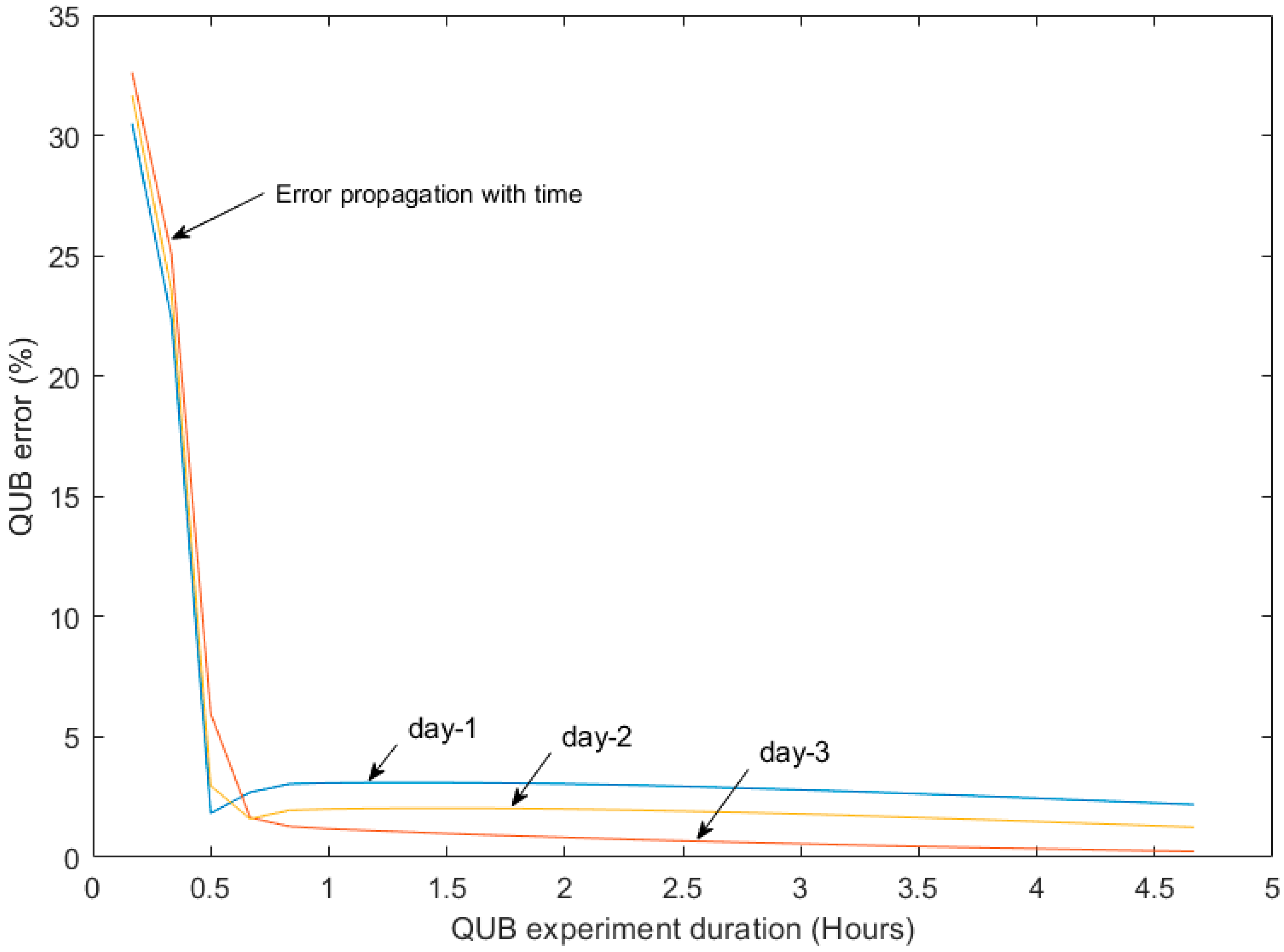
3.2.2. Time Duration

It is interesting to see that $H$-values with small errors could be obtained with QUB tests having short heating duration. This is evident from Figure 15 showing that $H_{QUB}$ value within $\pm 20\%$ of the reference value could be obtained during the first half hour of QUB experiment. The error curves however were very sensitive to power level if the duration of the experiment was short.

The variation in error with the time duration of QUB test could be further explored by performing QUB experiments with different time durations. The dependency of QUB errors with time was generated by repeating a QUB experiment with time duration ranging from 20 min to 5 h (Figure 16). It can be seen that initially the error was large ($30\%$) but it reduced significantly during the next twenty minutes. The error remains almost constant after $1$–$2$ h of the QUB experiment, which was in accordance with previously published results [11]. This behavior was explained by the important contribution of the exponentials corresponding to medium time constants ($1\dots 2$ h), which have significant coefficients [5].

3.2.3. Value of Power during the Experiment

It is evident from the plot of error curves (Figure 3) that variation in input power changes the output of the QUB method. The optimum power for QUB experiment on any day with reference to the initial power can be estimated by using [7]:

$$P_{optimum}=n H_{ref}\left(T_i-T_o\right),$$

(18)

where $n$ can vary from 1.7 to 3.3 [16].

The effect of variation of the optimum power could be investigated by generating error curves for the twin house with $\pm 20\%$ of the optimum power ($P_{optimum}$) value. In this case the error curves were almost vertical (Figure 17). The advantage of this behavior was that the variation in QUB error (with $\pm 20\%$ variation in power) was limited (maximum variation of $6\%$ in QUB error). For example, the QUB error would vary by 3% when the optimum power varied from 2100 to 2600 W (blue vertical line in Figure 17).

4. Influence of the Initially Assumed Value of the Overall Heat Loss Coefficient

Design of experiment can be used to estimate the optimum power for the QUB experiment that can give low errors [11]. The design of experiment (DOE) depends on the overall heat loss coefficient used, a quantity that depends on the stated or calculated value using building material properties. The stated or calculated value of the overall heat loss coefficient is not known accurately due to material property deterioration, missing insulation layers, moisture transfer and the quality of workmanship. It is therefore important to investigate how the results of the QUB method change when the overall heat loss coefficient value used in the design of the experiment is different from the real overall heat loss coefficient of building, which in general is larger than the designed value.

Three cases were studied in which the value of $H$ (used for the design of the experiment) and the real value of $H$ were different:

(1)

The outer wall insulation for design of QUB experiment was two times higher than of the real wall ($8\%$ error in assumed $H_{ref}$ compared to the real envelope).

(2)

The real wall insulation is completely missing whereas in the design of QUB experiment the outer wall has insulation ($50\%$ error in assumed $H_{ref}$ compared to the real envelope).

(3)

The real wall had no insulation and the roof insulation was smaller as compared to the wall and roof insulation used in the design of QUB experiment ($100\%$ error in assumed $H_{ref}$ compared to the real envelope).

For the cases discussed above, the a priori error is defined as the error when the real $H$-value was used for designing the experiment, whereas the a posteriori error is defined as the error when a supposed $H$-value (obtained, for example from building specifications), which is different of the real $H$-value, was used for designing the experiment. Figure 18 shows the results of 32 QUB experiments conducted on different days. The results show that when $8\%$ error of $H$-value was used in the design of the experiment (Figure 18a), the increase in a posteriori error was not significant (shown by the blue bar slightly higher than the red bar).

Figure 18b shows that with no outer wall insulation ($H_{ref}$ error of 50%) the a posteriori error was higher than the a priori error, with a median of a posteriori errors $10\%$ as compared to median error of 6% for a priori errors. The majority of errors still lied within $\pm 15\%$. In case of no wall insulation and reduced roof insulation (${\mathrm{H}}_{\mathrm{ref}}$ error of 100%) the a posteriori error was significantly higher as compared to a priori error, with a median of a posteriori errors of $16\%$ as compared to a priori median error of 8% (Figure 18c). Nevertheless, in this case the error made with the QUB method (median error of 16%) was significantly smaller than the error made on the initial estimate of the overall heat loss coefficient (100%).

This also means that, in practice, the experimentalist will clearly notice that “something went wrong” in the sense that the measured value of the heat loss coefficient is very different from the assumed value (median difference being 100% − 16% = 84%). The experimentalist can then suspect that there is an important gap between the theoretical design of the building and its actual state. This could also trigger another QUB experiment, using for the design of experiment the measured value of the heat loss coefficient instead of the theoretical (or stated by design) value. In this case, the measured and the assumed values would be much closer, confirming the important gap between theoretical and actual thermal performance.

5. Conclusions

In this work, QUB numerical experiments were performed on a verified model of a real house at different levels of power, starting time, time duration, initial and boundary conditions. The weather data of forty days was used to simulate numerical QUB experiments. The following conclusions could be drawn from the results of the numerical QUB experiments:

• Heating building with steady state power before the experiment improved QUB results. The error curves show a large error when there was no initial power before the QUB experiment. The error curves converged to smaller error when the building was supplied with power before the experiment.
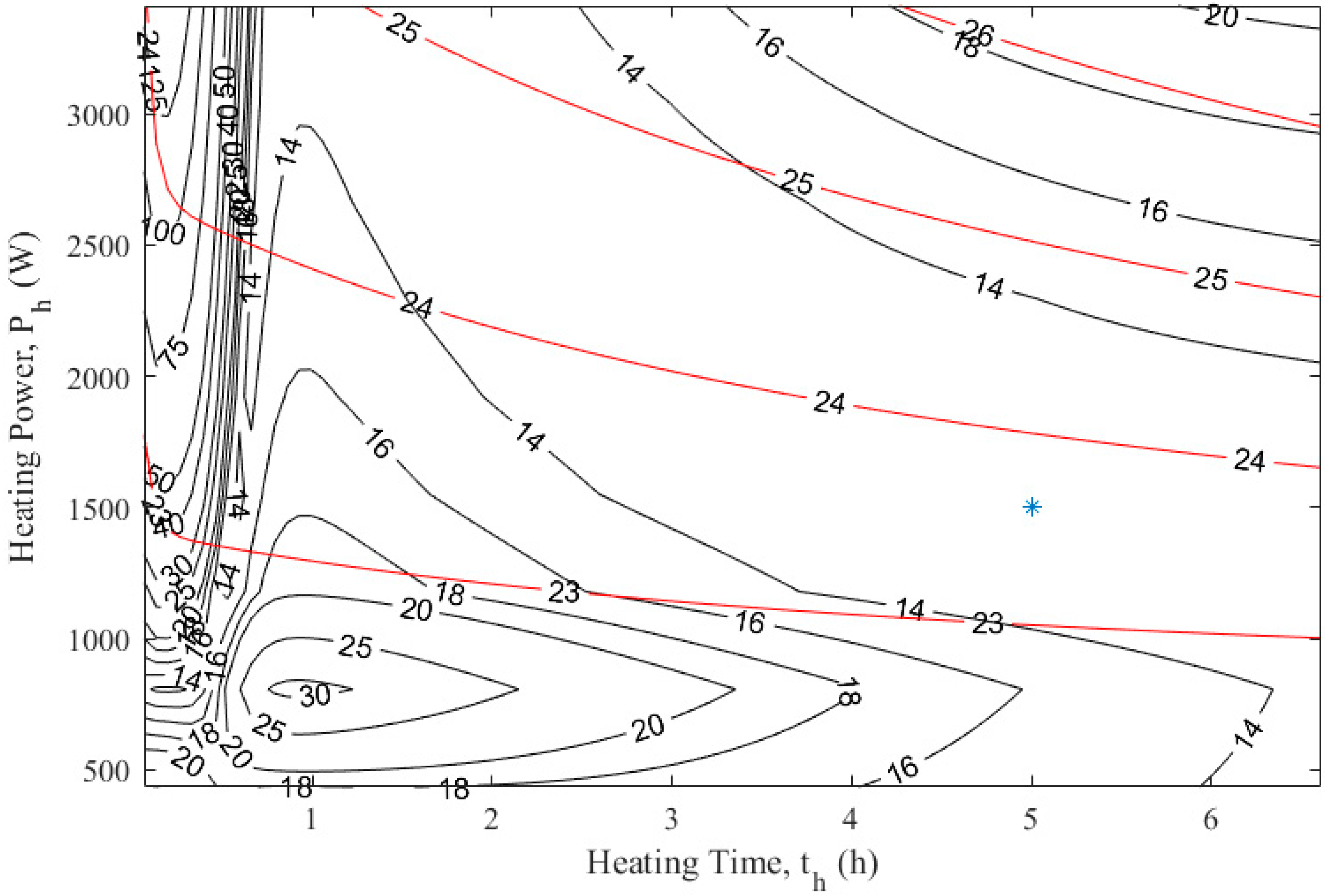
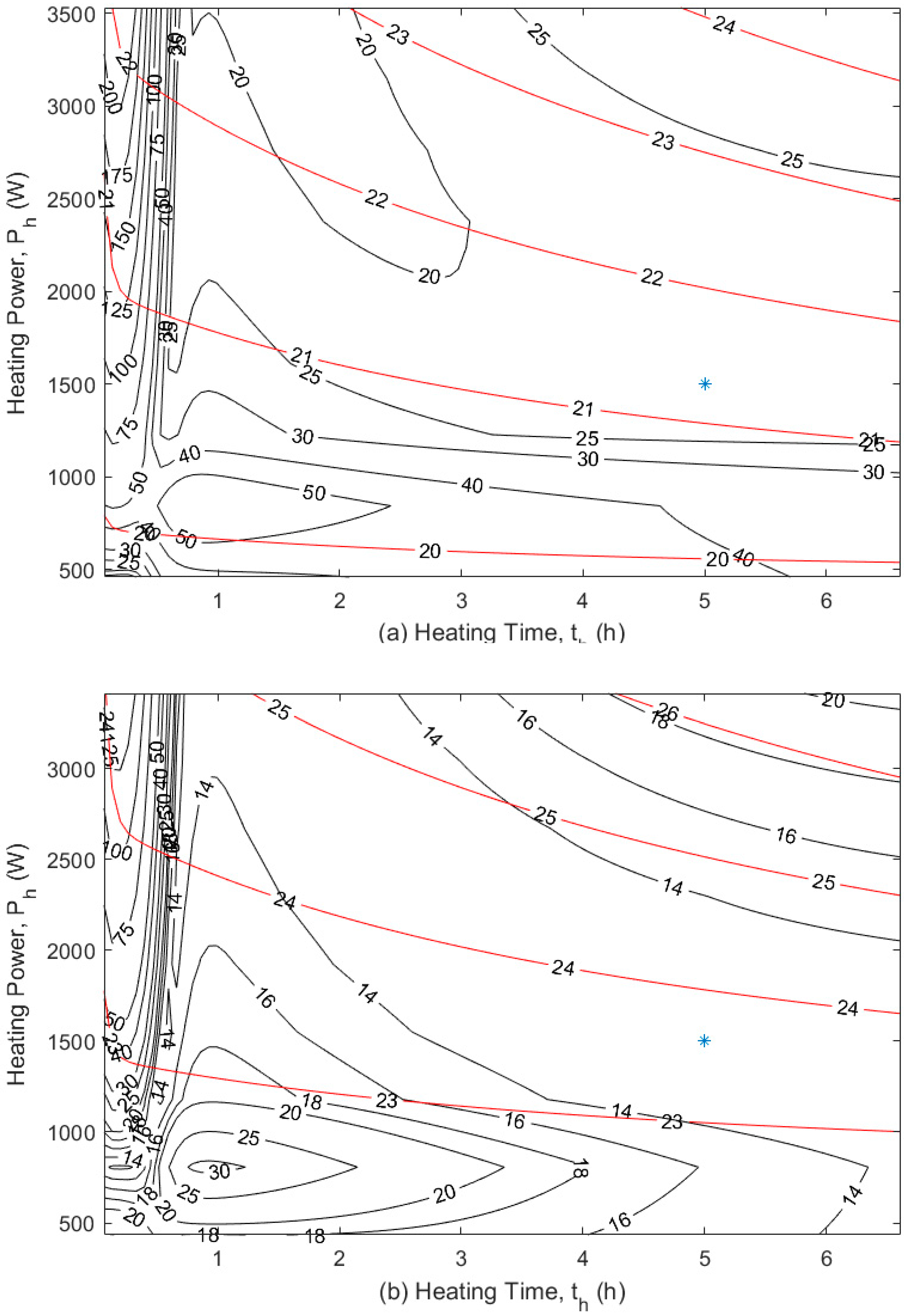
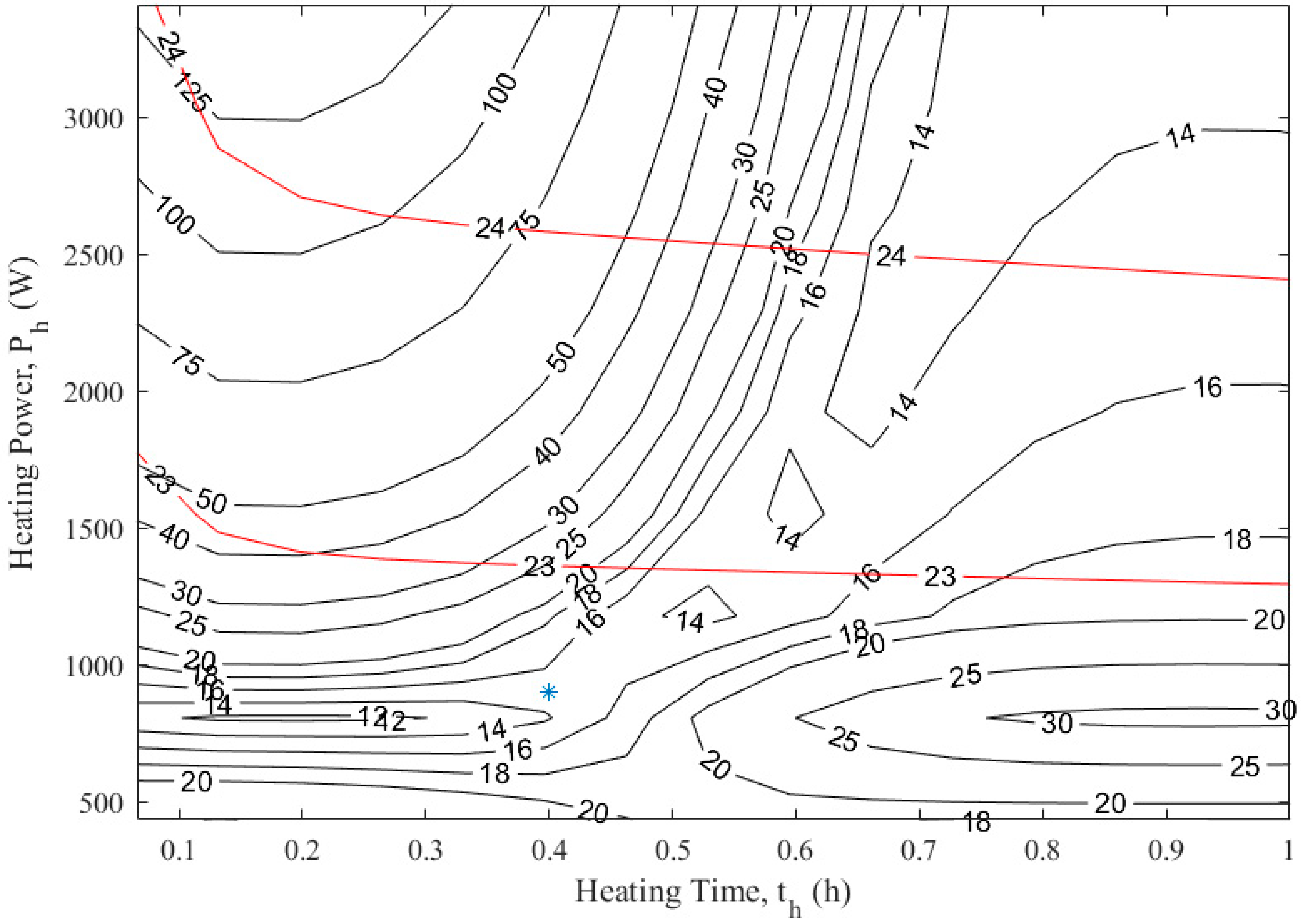
• $H_{QUB}$ values within $\pm 20\%$ of the steady state value could be obtained with short durations of the QUB experiment (0.2–1 h). However, the measured overall heat loss coefficient, $H_{QUB}$, was sensitive to power variation during the first hour. The error curves were less sensitive to variation in heating power if the QUB experiment was longer than $2$ h.
• The starting time of the QUB experiment before or after the sunset affected the results. A QUB experiment half an hour before the sunset gave an error of 14% that was reduced to 11% when the experiment was conducted one hour after the sunset.
• Comparison of QUB results for sunny and cloudy days revealed that at a given power and time duration of the QUB experiment the results on cloudy days showed less variation as compared to sunny days.
• QUB errors on sunny days were due to solar radiation absorbed by the walls of the building. The absorbed solar radiation contributes as a delayed heat input to the evolution of air temperature during heating phase. This paper proposed a method to estimate the delayed solar radiation and to correct the input power during the heating phase. The solar correction factor, when added to the heating power $P_1$ in the QUB expression, reduced the error by 2%.
• A $\pm 20\%$ variation in power used for QUB experiment as per recommend power level $P_{optimum}=2H_{ref}\left(T_i-T_o\right)$ could change the error by 3%–4%.
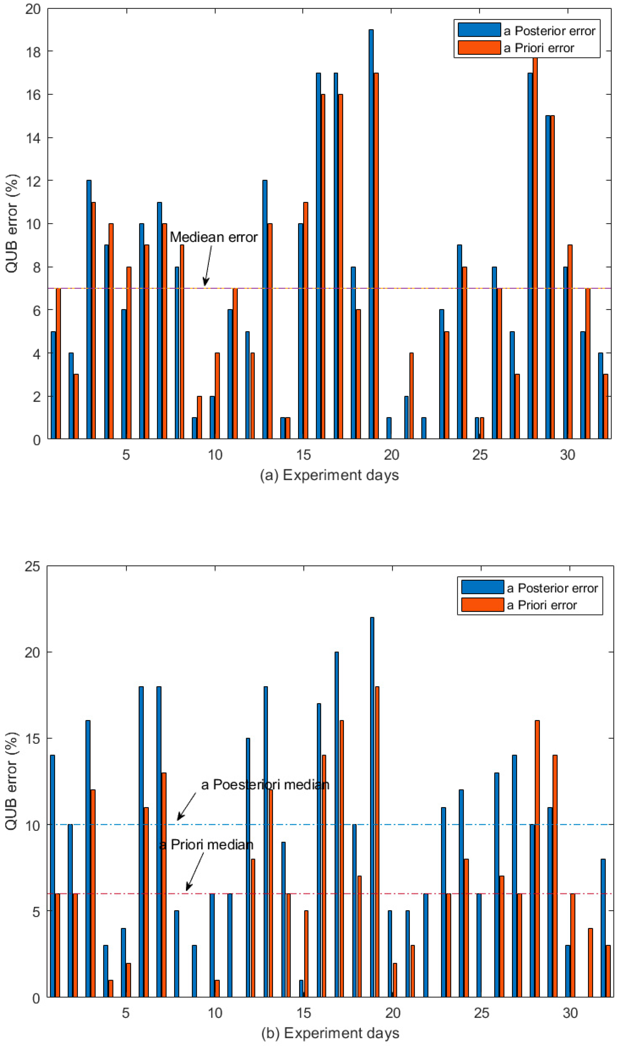
• It is possible that the overall heat loss coefficient value $H_{ref}$ used for calculation of optimum power for QUB experiment is not known with accuracy, e.g., there may be a missing insulation layer inside the wall or the thickness of the real wall insulation may be higher than the stated value. To check the robustness of QUB method, three scenarios were replicated to perform a posteriori error analysis:

  -

  The real outer wall insulation was twice the assumed value: the real $H_{ref}$ value of the house was $8\%$ less than the value used for QUB experiment design. QUB method (without knowing the real situation) responded well to the changed $H$-value. The error remained well within 15% for most of the days of QUB experiment.

  -

  The real outer wall insulation was missing (50% change in value as compared to the assumed $H$-value for QUB method): QUB method, without knowing the real condition of outer wall, responded with 4% increase in error compared to the situation when the real condition of the outer wall was known. The error remained within $\pm 20\%$ for most of the days of QUB experiment.

  -

  The real outer wall insulation was missing and the roof insulation was reduced (100% changed value as compared to the assumed $H$-value for the QUB method). Though the QUB method responded to the changed situation, the error increased significantly ($12.5\%$). Still, even in this extreme case, we noted that the error made with the QUB method was significantly smaller than that error made originally. In this situation, although the accuracy of the method was deteriorated, the method still clearly showed the important fact that the assumed value of heat loss coefficient was far smaller than the true one.

References

1. Coakley, D.; Raftery, P.; Keane, M. A review of methods to match building energy simulation models to measured data. Renew. Sustain. Energy Rev. 2014, 37, 123–141. [Google Scholar] [CrossRef] [Green Version]
2. Deconinck, A.H.; Roels, S. Comparison of characterisation methods determining the thermal resistance of building components from onsite measurements. Energy Build. 2016, 130, 309–320. [Google Scholar] [CrossRef] [Green Version]
3. Menezes, A.C.; Cripps, A.; Bouchlaghem, D.; Buswell, R. Predicted vs. actual energy performance of non-domestic buildings: Using post-occupancy evaluation data to reduce the performance gap. Appl. Energy 2012, 97, 355–364. [Google Scholar] [CrossRef] [Green Version]
4. Kosmina, L. Guide to In-Situ U-Value Measurement of Walls in Existing Dwellings In-Situ Measurement of U-Value. BRE. 2016. Available online: https://www.bre.co.uk/filelibrary/In-situ-measurement-of-thermal-resistance-and-thermal-transmittance-FINAL.pdf (accessed on 19 November 2019).
5. Ghiaus, C.; Alzetto, F. Design of experiments for Quick U-building method for building energy performance measurement. J. Build. Perform. Simul. 2019, 12, 465–479. [Google Scholar] [CrossRef]
6. Fabrizio, E.; Monetti, V. Methodologies and advancements in the calibration of building energy models. Energies 2015, 8, 2548–2574. [Google Scholar] [CrossRef] [Green Version]
7. Stamp, S.; Altamirano-Medina, H.; Lowe, R. Assessing the Relationship between Measurement Length and Accuracy within Steady State Co-Heating Tests. Buildings 2017, 7, 98. [Google Scholar] [CrossRef] [Green Version]
8. Strachan, P.; Heusler, I.; Kersken, M.; Jiménez, M.J. Empirical Whole Model Validation Modelling Specification Validation of Building Energy Simulation Tools. IEA EBC Annex 2016, 58. [Google Scholar]
9. Bouchié, R.; Alzetto, F.; Brun, A.; Boisson, P.; Thébault, S. Short methodologies for in-situ assessment of the intrisinc thermal performance of the building envelope. In Proceedings of the Sustainable Places, Nice, France, 1–3 October 2014. [Google Scholar]
10. Subbarao, K. PSTAR: Primary and Secondary Terms Analysis and Renormalization: A Unified Approach to Building Energy Simulations and Short-Term Monitoring; Report SERI/TR-254-3347; Solar Energy Research Institute: Golden, CO, USA, 1988. [Google Scholar]
11. Thébault, S.; Bouchié, R. Refinement of the ISABELE method regarding uncertainty quantification and thermal dynamics modelling. Energy Build. 2018, 178, 182–205. [Google Scholar] [CrossRef]
12. Alzetto, F.; Gossard, D.; Pandraud, G. Mesure rapide du coefficient de perte thermique des bâtiments. In Proceedings of the Congrès Sciences et Technique Ecobat, Paris, France, 19–20 March 2014; pp. 19–20. [Google Scholar]
13. Pandraud, G.; Didier, G.; Alzetto, F. Experimental optimization of the QUB method. In Proceedings of the IEA–EBC Annex 58, 6th Expert Meeting, Ghent, Belgium, 14–16 April 2014. [Google Scholar]
14. Meulemans, J.; Alzetto, F.; Farmer, D.; Gorse, C. QUB/e: A novel transient experimental method for in situ measurements of the thermal performance of building fabrics. In Proceedings of the International Sustainable Ecological Engineering Design for Society (SEEDS) Conference, Leeds, UK, 14–15 September 2016; pp. 14–15. [Google Scholar]
15. Alzetto, F.; Didier, G.; Pandraud, G. Mesure rapide du coefficient de perte thermique des bâtiment. In Proceedings of the Congrès écobat Sciences et Techniques, Porte de Versailles, Pavilion 7, France, 19–20 March 2014; pp. 1–10. [Google Scholar]
16. Alzetto, F.; Pandraud, G.; Fitton, R. QUB: A fast dynamic method for in-situ measurement of the whole building heat loss. Energy Build. 2018, 174, 124–133. [Google Scholar] [CrossRef]
17. Pandraud, G.; Fitton, R. QUB: Validation of a Rapid Energy Diagnosis Method for Buildings. In Interanational Energy Agency Annex 58; University of Salford: Manchester, UK, 2014; pp. 1–6. [Google Scholar]
18. Strachan, P.; Svehla, K.; Heusler, I.; Kersken, M. Whole model empirical validation on full-scale building. J. Build. Perform. Simul. 2015, 9, 331–350. [Google Scholar] [CrossRef] [Green Version]
19. Balakrishnan, V. System identification: Theory for the user (second edition). Automatica 2002, 38, 375–378. [Google Scholar] [CrossRef]
Figure 1. The quick U-building (QUB) experiment principles and steps [13].
Energies 13 00284 g001
Figure 2. The ground floor of the house layout and dimensions (in cm).
Energies 13 00284 g002
Figure 3. Design of the QUB experiment: (a) heating power and time duration: error curves of the overall heat loss coefficient (black) and internal temperature (red); the blue star shows the error when the experiment is performed at 1500 W and 5 h duration for the each phase of the QUB experiment and (b) the exponential response of seven zones of the house for 1500 W and 5 h: fall of temperature during the two stages of QUB experiments (dotted line), weighted average temperature rise during heating (the black circles) and weighted average temperature fall during cooling (pink).
Energies 13 00284 g003
Figure 4. (a) Overall heat loss coefficient obtained with the QUB experiment obtained for 40 days with weather data obtained by International Energy Agency (IEA), EBC Annex-58. The dashed red lines show a range of ±20% of the reference steady state value. (b) Global horizontal radiation. (c) Outdoor temperature during 40 days of QUB experiment.
Energies 13 00284 g004
Figure 5. Error (blue star) when the experiment is performed half an hour before the sunset time (at 1500 W and 5 h of heating); error of measured overall heat loss coefficient (black curves), indoor temperature (red curves).
Energies 13 00284 g005
Figure 6. Results (blue star) when the experiment is performed one hour after the sunset (at 1500 W and 5 h of heating); error of overall heat loss coefficient (black curves), indoor temperature (red curves).
Energies 13 00284 g006
Figure 7. QUB value variation as a function of day type: sunny, partly cloudy and cloudy days. Dashed horizontal line (red) is the steady state reference value.
Energies 13 00284 g007
Figure 8. Convergence of the QUB test when the experiment is repeated without solar radiations (blue circles) and with solar radiations (black asterisk). In absence of solar radiations (blue circles) the QUB test settles at a value closer to H r e f . Blue dashed line the reference/steady state over all heat transfer coefficient ( H r e f ), upper dashed red line (+20% H r e f ) and lower dashed red line (−20% H r e f ).
Energies 13 00284 g008
Figure 9. Temperature evolution during the QUB heating phase with no solar radiation (in orange) and with solar radiation (in blue).
Energies 13 00284 g009
Figure 10. QUB experiment with (a) indoor temperature evolution as a function of solar radiation, outdoor temperature and heater power and (b) temperature evolution as a function of outdoor temperature, heater power and a controller.
Energies 13 00284 g010
Figure 11. Temperature evolution during the QUB heating phase with no solar radiations and controller heat (orange line) and with solar radiations (blue).
Energies 13 00284 g011
Figure 12. The error with solar correction (black asterisk) smaller (closer to H r e f reference value) and no solar correction (blue asterisks) further from the reference value. Blue dashed line the reference/steady state over all heat transfer coefficient ( H r e f ), upper dashed red line (+20% H r e f ) and lower dashed red line (−20% H r e f ).
Energies 13 00284 g012
Figure 13. QUB error curves for the experimental house (a) no initial power before the experiment, the curves move towards increased error (b) initial power before the experiment, the curves converge, red curves show the indoor air temperature and black curve show the error curves.
Energies 13 00284 g013
Figure 14. QUB values obtained for simulations for forty days (a) no initial power before the QUB experiment and (b) initial power before QUB experiment. Blue dashed line the reference/steady state over all heat transfer coefficient ( H r e f ), upper dashed red line (+20% H r e f ) and lower dashed red line (−20% H r e f ).
Energies 13 00284 g014
Figure 15. QUB error curves (black) and indoor temperature curves (red) during the first 1.5 h of the QUB experiment (heating phase).
Energies 13 00284 g015
Figure 16. Variation of QUB error with change in time duration of the QUB experiment.
Energies 13 00284 g016
Figure 17. QUB errors generated with variation of the optimum power: error curves (black) and indoor temperature (red). The blue vertical line shows error for QUB experiments at different levels of power but for the same duration of the experiment.
Energies 13 00284 g017
Figure 18. A posteriori error analysis for three case studies: (a) outer wall insulation is reduced (8% error in H-value), (b) outdoor wall insulation is completely removed (50% error in H-value) and (c) outdoor wall insulation removed and roof insulation reduced (100% error in H-value). Red bars show error with real envelope and blue bars show QUB error with assumed envelope.
Energies 13 00284 g018aEnergies 13 00284 g018b