A Study on the Operational Condition of a Ground Source Heat Pump in Bangkok Based on a Field Experiment and Simulation


 , , and
Abstract
1. Introduction
- (1)
- An experimental investigation was conducted by using the same pilot facility in the previous study in Bangkok [11] to elucidate the efficiency of a GSHP and ASHP according to the heat sink temperatures.
- (2)
- A simulation was conducted that utilized the analytical solution of the heat conduction equation to predict the subsurface temperature increase due to the GSHP operation over the long term.
2. Materials and Methods
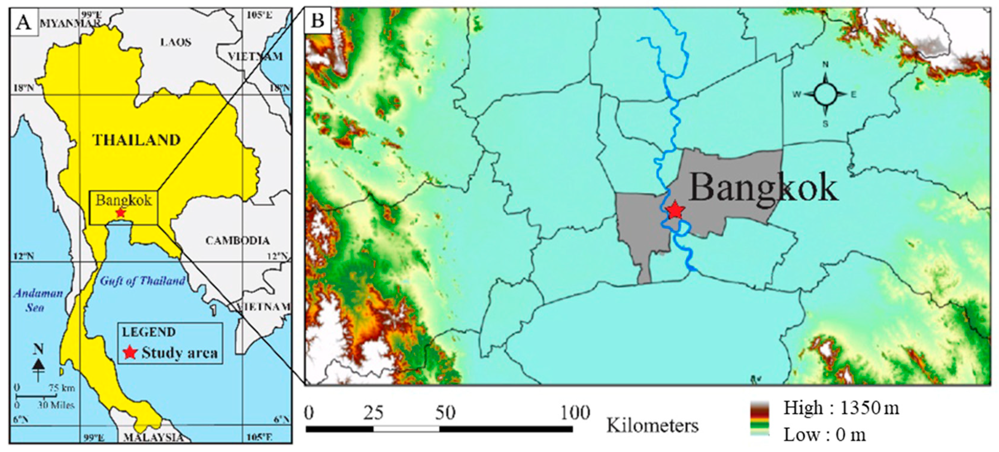
2.1. Experimental Investigation
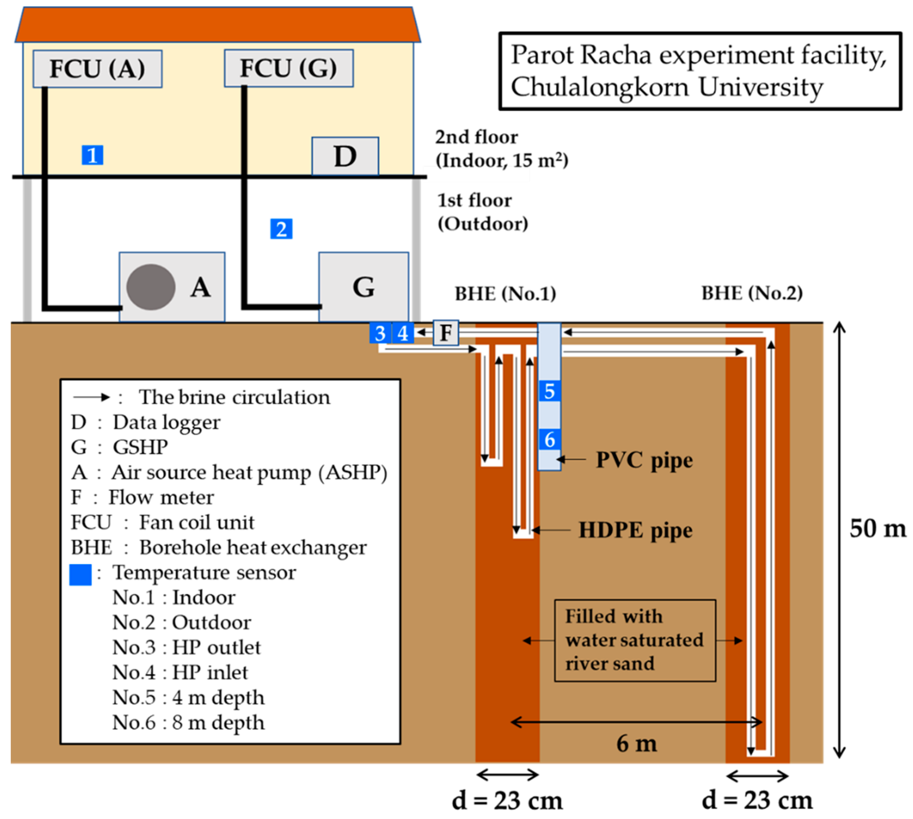
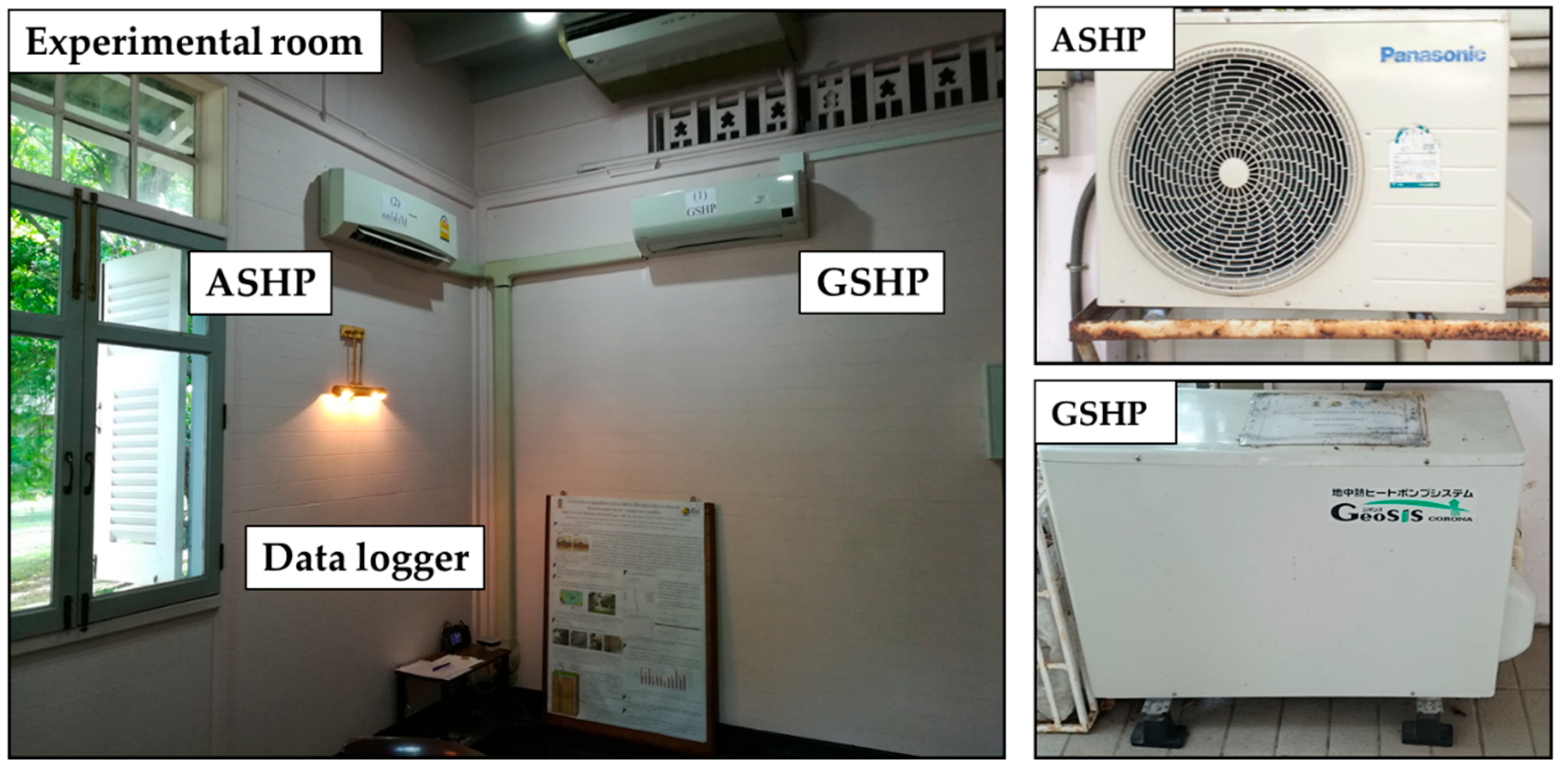
2.1.1. Description of the Experiment Facility
Borehole Heat Exchanger (BHE)
Heat Pump (HP)
Data Acquisition System
2.1.2. Experimental Conditions
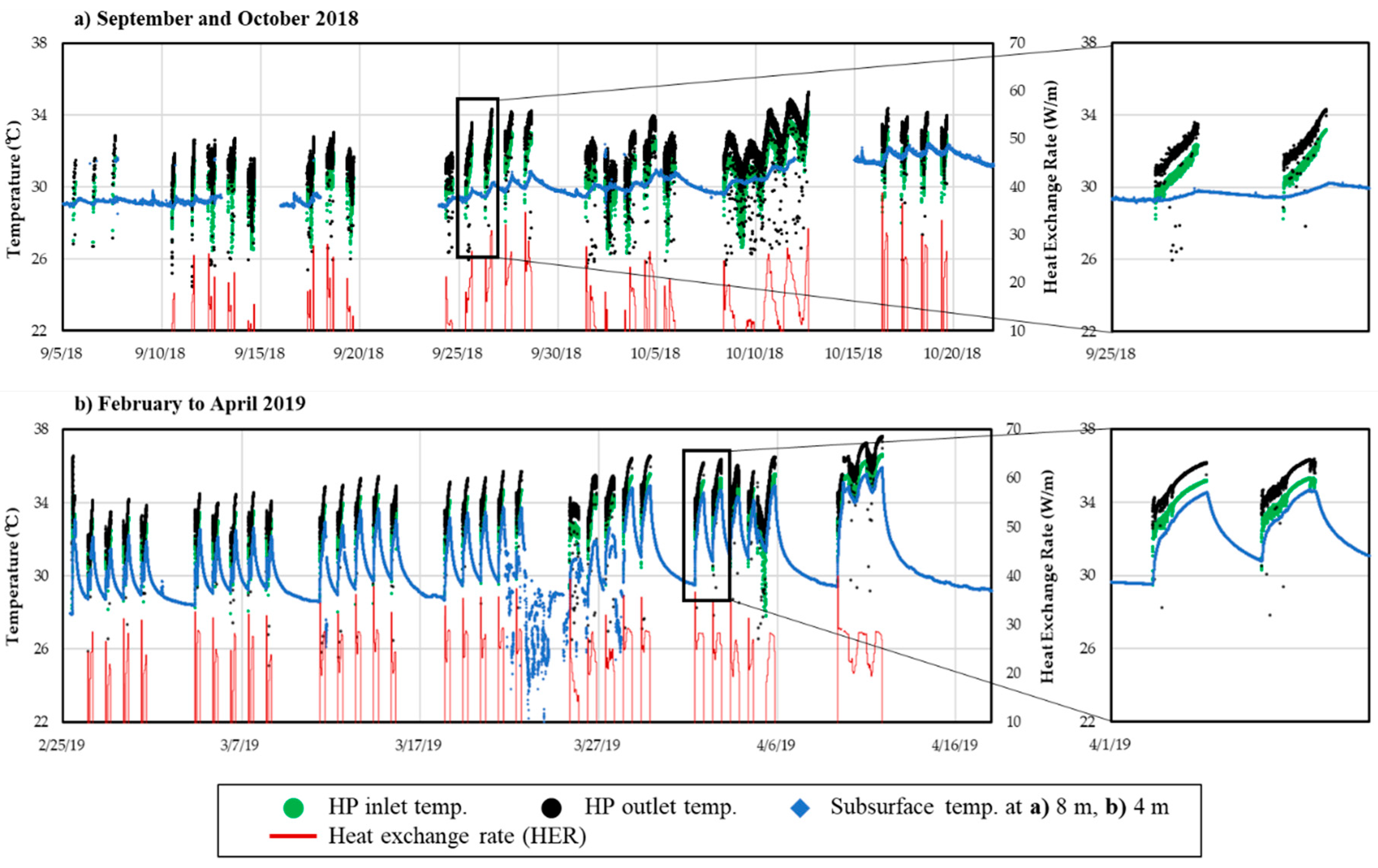
September and October 2018 (Rainy Season)
February to April 2019 (Hot and Dry Season)
2.1.3. Analysis on the GSHP and ASHP Operation
Heat Exchange Rate Per Unit Length of BHE (HER)
Cooling Load
System Coefficient of Performance (Sys-COP)
2.2. Simulation of Long-Term GSHP Operation
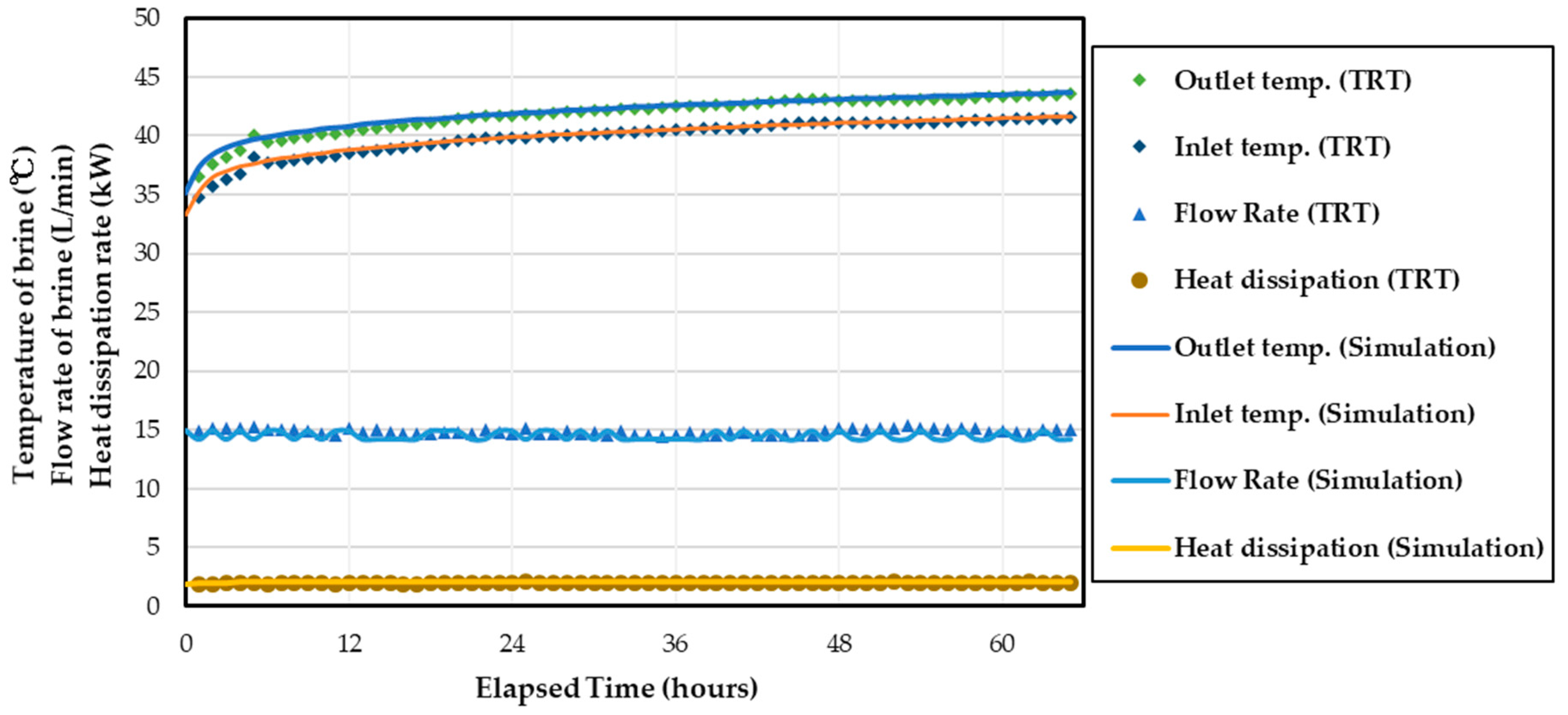
2.2.1. Determining the Subsurface Thermal Properties
2.2.2. Simulation Parameters
3. Results and Discussion
3.1. Experimental Investigation
3.1.1. Subsurface Temperature Change
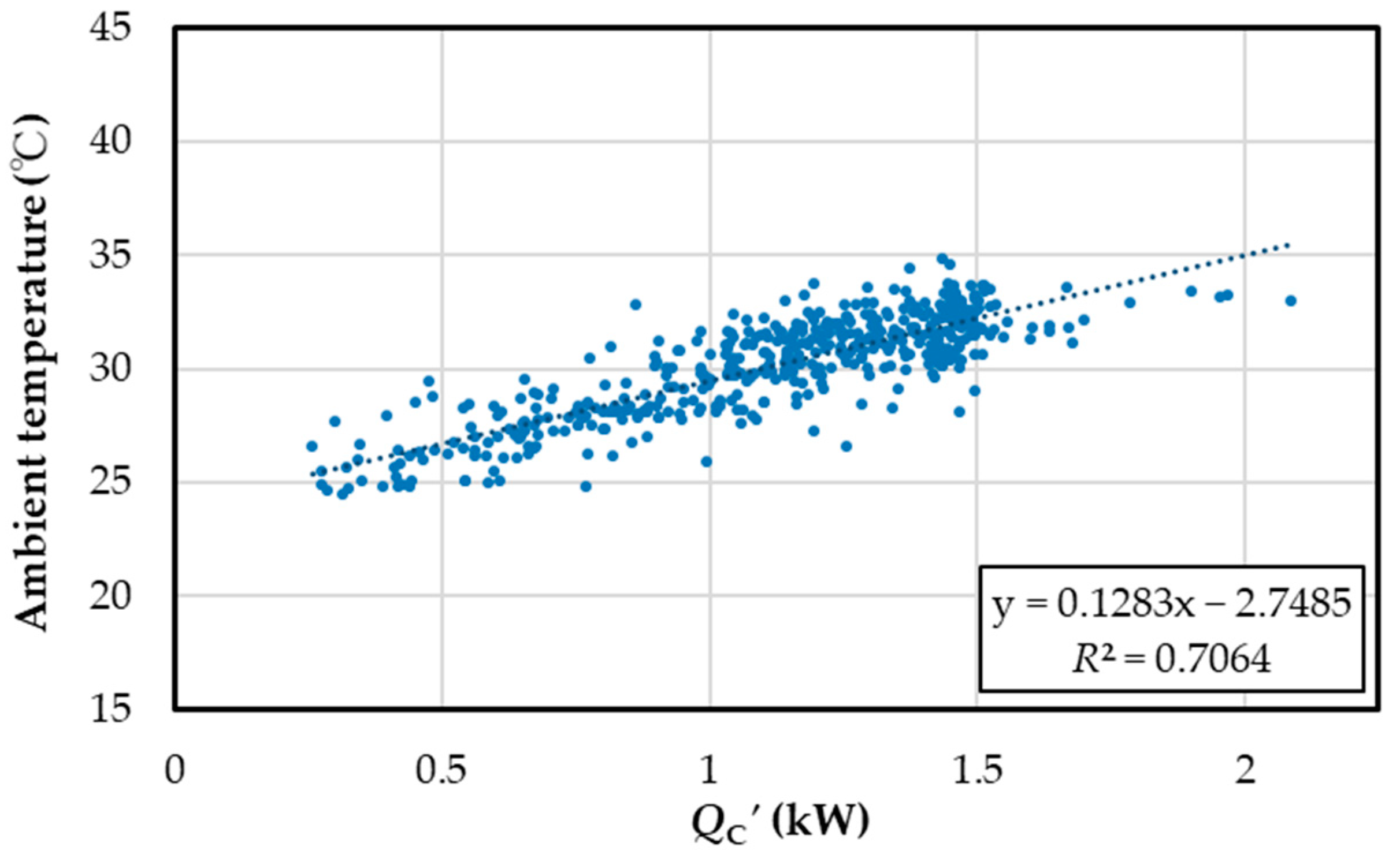
3.1.2. Performance Analysis of the Heat Source Temperature
3.2. Simulation of Long-Term GSHP Operation
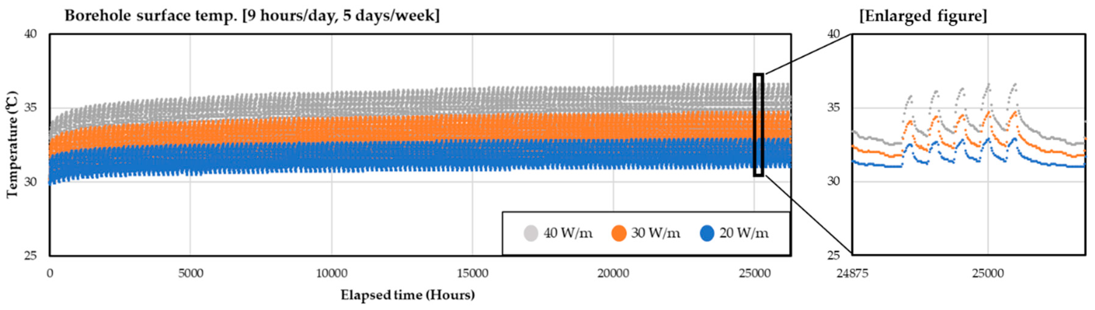
- (1)
- When operating the GSHP 5 days per week:When the HER was 20 W/m, operating the GSHP for less than 14 h per day;When the HER was 30 W/m, operating the GSHP for less than 9 h per day;When the HER was 40 W/m, operating the GSHP for less than 5 h per day.
- (2)
- When operating the GSHP every day:When the HER was 20 W/m, operating the GSHP for less than 14 h per day;When the HER was 30 W/m, operating the GSHP for less than 5 h per day.
4. Conclusions
Author Contributions
Funding
Acknowledgments
Conflicts of Interest
References
- IRENA. Renewable Energy Outlook: Thailand; International Renewable Energy Agency: Abu Dhabi, UAE, 2017; p. 45. ISBN 978-9-29-260035-8. [Google Scholar]
- Office of Natural Resources and Environmental Policy and Planning. Available online: https://www4.unfccc.int/sites/submissions/INDC/Published%20Documents/Thailand/1/Thailand_INDC.pdf (accessed on 23 July 2019).
- Office of Natural Resources and Environmental Policy and Planning. Thailand’s Second National Communication under the United Nations Framework Convention on Climate Change; Ministry of Natural Resources and Environment: Bangkok, Thailand, 2010; pp. 45–46. ISBN 978-9-74-286865-9.
- Sivak, M. Potential energy demand for cooling in the 50 largest metropolitan areas of the world: Implications for developing countries. Energy Policy 2009, 37, 1382–1384. [Google Scholar] [CrossRef]
- Yungchareon, V.; Limmeechokchai, B. Energy Analysis of the Commercial Sector in Thailand: Potential Savings of Selected Options in Commercial Buildings. In Proceedings of the SEE International Conference, Petchaburi, Thailand, 19–21 May 2004; pp. 496–501. [Google Scholar]
- Chirarattananon, S.; Taweekun, J. A technical review of energy conservation programs for commercial and government buildings in Thailand. Energy Convers. Manag. 2003, 44, 743–762. [Google Scholar] [CrossRef]
- Sasada, M.; Takasugi, S.; Tateno, M. A Ground Source Heat Pump System in Central Tokyo; A Case Study of Retrofit for a Small Office Building. J. Jpn. Soc. Eng. Geol. 2011, 51, 265–272. [Google Scholar] [CrossRef]
- Urchueguía, J.F.; Zacares, M.; Corberán, J.M.; Montero, A.; Martos, J.; Witte, H. Comparison between the energy performance of a ground coupled water to water heat pump system and an air to water heat pump system for heating and cooling in typical conditions of the European Mediterranean coast. Energy Convers. Manag. 2008, 49, 2917–2923. [Google Scholar] [CrossRef]
- Brouwers, J.; Entrop, A.G. New Triplet Visions on Sustainable Building, Action for sustainability. In Proceedings of the 2005 World Sustainable Building Conference (on CD-Rom), Tokyo, Japan, 27–29 September 2005; pp. 4330–4335. [Google Scholar]
- Yasukawa, K.; Uchida, Y.; Tenma, N.; Taguchi, Y.; Muraoka, H.; Ishii, T.; Suwanlert, J.; Buapeng, S.; Nguyen, T.H. Groundwater temperature survey for geothermal heat pump application in tropical Asia. Bull. Geol. Surv. Jpn. 2009, 60, 459–467. [Google Scholar] [CrossRef]
- Chokchai, S.; Chotpantarat, S.; Takashima, I.; Uchida, Y.; Widiatmojo, A.; Yasukawa, K.; Charusiri, P. A Pilot Study on Geothermal Heat Pump (GHP) Use for Cooling Operations, and on GHP Site Selection in Tropical Regions Based on a Case Study in Thailand. Energies 2018, 11, 2356. [Google Scholar] [CrossRef]
- Widiatmojo, A.; Chokchai, S.; Takashima, I.; Uchida, Y.; Yasukawa, K.; Chotpantarat, S.; Charusiri, P. Ground-Source Heat Pumps with Horizontal Heat Exchangers for Space Cooling in the Hot Tropical Climate of Thailand. Energies 2019, 12, 1274. [Google Scholar] [CrossRef]
- Shimada, Y.; Kurishima, H.; Uchida, Y. Life Cycle Environmental Evaluation on Introduction of Ground Source Heat Pump in Bangkok, Thailand. J. Life Cycle Assess. Jpn. 2019, 15, 269–281. [Google Scholar]
- Safa, A.A.; Fung, A.S.; Kumar, R. Heating and cooling performance characterisation of ground source heat pump system by testing and TRNSYS simulation. Renew. Energy 2015, 83, 565–575. [Google Scholar] [CrossRef]
- Rybach, L.; Eugster, W.J. Sustainability aspects of geothermal heat pump operation, with experience from Switzerland. Geothermics 2010, 39, 365–369. [Google Scholar] [CrossRef]
- Michopoulos, A.; Zachariadis, T.; Kyriakis, N. Operation characteristics and experience of a ground source heat pump system with a vertical ground heat exchanger. Energy 2013, 51, 349–357. [Google Scholar] [CrossRef]
- Zhai, X.Q.; Yu, X.; Yang, Y.; Wang, R.Z. Experimental investigation and performance analysis of a ground-coupled heat pump system. Geothermics 2013, 48, 112–120. [Google Scholar] [CrossRef]
- Man, Y.; Yang, H.; Wang, J. Study on hybrid ground-coupled heat pump system for air-conditioning in hot-weather areas like Hong Kong. Appl. Energy 2010, 87, 2826–2833. [Google Scholar] [CrossRef]
- Kharseh, M.; Al-Khawaja, M.; Suleiman, M.T. Potential of ground source heat pump systems in cooling-dominated environments: Residential buildings. Geothermics 2015, 57, 104–110. [Google Scholar] [CrossRef]
- Sanner, B.; Hellström, G.; Spitler, J.; Gehlin, S. Thermal response test–current status and world-wide application. In Proceedings World Geothermal Congress; International Geothermal Association: Antalya, Turkey, 2005. [Google Scholar]
- Ingersoll, L.R.; Plass, H.J. Theory of the ground pipe heat source for the heat pump. Heat. Pip. Air Cond. 1948, 20, 119–122. [Google Scholar]
- Uchida, Y.; Fujii, H. First thermal response test in Southeast Asia. GSJ Chishitsu News 2018, 7, 156–158. [Google Scholar]
- Gehlin, S. Thermal Response Test: Method Development and Evaluation; Luleå Tekniska Universitet: Luleå, Sweden, 2002. [Google Scholar]
- Ingersoll, L.R.; Zabel, O.J.; Ingersoll, A.C. Heat Conduction with Engineering, Geological, and Other Applications; McGraw-Hill: New York, NY, USA, 1954. [Google Scholar]
- Nagano, K.; Katsura, T.; Takeda, S. Development of a design and performance prediction tool for the ground source heat pump system. Appl. Therm. Eng. 2006, 26, 1578–1592. [Google Scholar] [CrossRef]
- Katsura, T.; Nagano, K.; Takeda, S. Method of calculation of the ground temperature for multiple ground heat exchangers. Appl. Therm. Eng. 2008, 28, 1995–2004. [Google Scholar] [CrossRef]
- Katsura, T.; Nagano, K.; Narita, S.; Takeda, S.; Nakamura, Y.; Okamoto, A. Calculation algorithm of the temperatures for pipe arrangement of multiple ground heat exchangers. Appl. Therm. Eng. 2009, 29, 906–919. [Google Scholar] [CrossRef]
- Katsura, T.; Nagano, K. Simulation Tool for Ground-Source Heat Pump System with Multiple Ground Heat Exchangers. ASHRAE Trans. 2018, 124, 92–101. [Google Scholar]
- Ministry of Land, Infrastructure, Transport and Tourism, Japan. Available online: https://www.mlit.go.jp/common/001016159.pdf (accessed on 23 July 2019).
- Ito, S.; Takano, Y.; Miura, N.; Uchikawa, Y. Studies of a Heat Pump Using Water and Air Heat Sources in a Series: Performance in Cooling Operation. Trans. Jpn. Soc. Mech. Eng. Ser. B 2001, 67, 2089–2096. [Google Scholar] [CrossRef]
- Crawley, D.B.; Lawrie, L.K.; Pedersen, C.O.; Winkelmann, F.C. Energy plus: Energy simulation program. ASHRAE J. 2000, 42, 49–56. [Google Scholar]


| Detail | ASHP | GSHP |
|---|---|---|
| Brand | PANASONIC | CORONA |
| Model | CS-PC12QKT | CSH-C4000G |
| Rated cooling capacity (W) | 3600 | 4000 |
| Rated cooling COP | 3.5 | 4.0 |
| Refrigerant | R410A | |
| September and October 2018 (Rainy Season) | |||||
| September | 5th~11th | 9:00~12:00: ASHP | 12:00~15:00: GSHP | 15:00~22:00: ASHP | |
| 12th~19th | 8:00~12:00: GSHP | 12:00~15:00: GSHP+ASHP | 15:00~16:00: GSHP | ||
| 24th~28th | 8:00~16:00: GSHP | ||||
| October | 1st~5th | 9:00~12:00: GSHP | 12:00~15:00: GSHP+ASHP | 15:00~22:00: GSHP | |
| 8th~12th | 24 Hours Operation: GSHP | ||||
| 16th~19th | 9:00~10:00: GSHP | 10:00~12:00: ASHP | 12:00~16:00: GSHP | 16:00~22:00: ASHP | |
| February to April 2019 (Hot and Dry Season) | |||||
| February | 26th~1st | 9:00~10:00: GSHP | 10:00~12:00: ASHP | 12:00~16:00: GSHP | 16:00~21:00: ASHP |
| March | 4th~8th | ||||
| 11th~15th | 9:00~16:00: GSHP | 16:00~21:00: ASHP | |||
| 18th~22nd | |||||
| 25th~29th | 9:00~21:00: GSHP | ||||
| April | 1st~5th | ||||
| 9th~11th | 24 Hours Operation: GSHP | ||||
| Nomenclature | Subscripts | ||
|---|---|---|---|
| C | specific heat (J/(kg °C)) | ashp | air source heat pump |
| COP | coefficient of performance (-) | b | brine |
| E | electric power (W) | c | cooling load |
| H | hydraulic head (m) | com | compressor |
| HER | heat exchange rate (W/m) | fan | fan (ASHP condensor) |
| L | length of BHE (m) | fcu | fan coil unit |
| m | flow rate (m3/min) | gshp | ground source heat pump |
| Q | thermal energy rate (W) | h | heat dissipation |
| r | radius (m) | in | heat pump inlet |
| Sys-COP | system coefficient of performance (-) | m | motor |
| t | time | out | heat pump outlet |
| T | temperature (°C) | p | pump |
| Greek symbols | s | subsurface soil | |
| λ | thermal conductivity (W/(m K)) | to | total |
| μ | efficiency (-) | ||
| ρ | density (kg/m3) |
| The specifications of BHE No. 2 | The type of BHE | Single U-tube |
| Brine | Water | |
| Diameter (m) | 0.23 | |
| Depth (m) | 50 | |
| Type of backfill material | Water saturated river sand | |
| Backfill material thermal conductivity (W/(m K)) | 2.0 | |
| The specifications of U-tube pipe | Material | HDPE |
| Outer diameter (mm) | 32 | |
| Inner diameter (mm) | 26 | |
| U-tube pipe thermal conductivity (W/(m K)) | 0.38 | |
| Subsurface soil thermal properties | Effective thermal conductivity (W/(m K)) | 1.82 |
| Heat capacity (kJ/(m3 K)) | 2600 | |
| The initial average temperature (°C) | 29.5 |
| HER | Operation Time per Day (5 days/week) | 90th Percentile Value Temp. at HP Inlet (°C) | Maximum Temp. at HP Inlet (°C) |
|---|---|---|---|
| 20 W/m | 5 h | 32.9 | 33.9 |
| 9 h | 34.7 | 35.2 | |
| 14 h | 36.1 | 36.5 | |
| 30 W/m | 5 h | 35.1 | 36.7 |
| 9 h | 37.9 | 38.6 | |
| 14 h | 40.1 | 40.6 | |
| 40 W/m | 5 h | 37.4 | 39.5 |
| 9 h | 41.3 | 42.2 | |
| 14 h | 44.3 | 45.1 | |
| Operation Time Per Day (Everyday) | |||
| 20 W/m | 5 h | 33.8 | 34.2 |
| 9 h | 35.5 | 35.7 | |
| 14 h | 37.1 | 37.3 | |
| 30 W/m | 5 h | 36.5 | 37.2 |
| 9 h | 39.2 | 39.5 | |
| 14 h | 41.7 | 42 | |
| 40 W/m | 5 h | 39.3 | 40.2 |
| 9 h | 43 | 43.4 | |
| 14 h | 46.7 | 47.1 |
© 2020 by the authors. Licensee MDPI, Basel, Switzerland. This article is an open access article distributed under the terms and conditions of the Creative Commons Attribution (CC BY) license (http://creativecommons.org/licenses/by/4.0/).
Share and Cite
Shimada, Y.; Uchida, Y.; Takashima, I.; Chotpantarat, S.; Widiatmojo, A.; Chokchai, S.; Charusiri, P.; Kurishima, H.; Tokimatsu, K. A Study on the Operational Condition of a Ground Source Heat Pump in Bangkok Based on a Field Experiment and Simulation. Energies 2020, 13, 274. https://doi.org/10.3390/en13010274
Shimada Y, Uchida Y, Takashima I, Chotpantarat S, Widiatmojo A, Chokchai S, Charusiri P, Kurishima H, Tokimatsu K. A Study on the Operational Condition of a Ground Source Heat Pump in Bangkok Based on a Field Experiment and Simulation. Energies. 2020; 13(1):274. https://doi.org/10.3390/en13010274
Chicago/Turabian StyleShimada, Yutaro, Youhei Uchida, Isao Takashima, Srilert Chotpantarat, Arif Widiatmojo, Sasimook Chokchai, Punya Charusiri, Hideaki Kurishima, and Koji Tokimatsu. 2020. "A Study on the Operational Condition of a Ground Source Heat Pump in Bangkok Based on a Field Experiment and Simulation" Energies 13, no. 1: 274. https://doi.org/10.3390/en13010274
APA StyleShimada, Y., Uchida, Y., Takashima, I., Chotpantarat, S., Widiatmojo, A., Chokchai, S., Charusiri, P., Kurishima, H., & Tokimatsu, K. (2020). A Study on the Operational Condition of a Ground Source Heat Pump in Bangkok Based on a Field Experiment and Simulation. Energies, 13(1), 274. https://doi.org/10.3390/en13010274