Optimization of Construction Duration and Schedule Robustness Based on Hybrid Grey Wolf Optimizer with Sine Cosine Algorithm

Abstract

Construction duration and schedule robustness are of great importance to ensure efficient construction. However, the current literature has neglected the importance of schedule robustness. Relatively little attention has been paid to schedule robustness via deviation of an activity’s starting time, which does not consider schedule robustness via structural deviation caused by the logical relationships among activities. This leads to a possibility of deviation between the planned schedule and the actual situation. Thus, an optimization model of construction duration and schedule robustness is proposed to solve this problem. Firstly, duration and two robustness criteria including starting time deviation and structural deviation were selected as the optimization objectives. Secondly, critical chain method and starting time criticality (STC) method were adopted to allocate buffers to the schedule in order to generate alternative schedules for optimization. Thirdly, hybrid grey wolf optimizer with sine cosine algorithm (HGWOSCA) was proposed to solve the optimization model. The movement directions and speed of grey wolf optimizer (GWO) was improved by sine cosine algorithm (SCA) so that the algorithm’s performance of convergence, diversity, accuracy, and distribution improved. Finally, an underground power station in China was used for a case study, by which the applicability and advantages of the proposed model were proved.

1. Introduction

Effective schedule management is becoming increasingly significant because of its social and economic benefits. Optimization is an important issue in schedule management. Both construction duration and schedule robustness, the latter of which is the schedule’s ability to resist duration increases due to interference, are necessary to be taken as the optimization objectives. However, schedule robustness is rarely considered as an optimization objective in current research, which causes deviations between the actual schedule and the planned one. Therefore, it is necessary to conduct optimization of construction duration and schedule robustness.

The basics of optimization is to determine objectives. Besides the objective of construction duration, it is also necessary to determine appropriate robustness criteria as optimization objectives. A few general robustness criteria have been defined to measure schedule robustness, including the summation of each activity’s free float [1], ratio of each activity’s free float and duration [2,3], linear weighted summation of the total free float [4], and linear weighted summation of the time deviations [5]. For complex construction projects, the schedule is established by breaking down the construction project into basic units (which are called activities) and determining the starting time of activities and logical relationships among them. Starting time of activities and logical relationships among them are two indispensable parts, thus the schedule robustness should be measured from these two aspects. But, in the very few multi-objective optimization studies considering both construction duration and schedule robustness, only the starting time deviation is taken as an objective [6]. The neglect of schedule robustness from the perspective of logical relationships among activities—that is, when structural deviation isn’t taken as an objective—will cause the construction site to be chaotic. Therefore, it is practical and necessary to take construction duration, starting time deviation, and structural deviation as the optimization objectives.

The method to improve schedule robustness is a necessary condition to generate alternative schedules for optimization. Buffer allocation methods are proven effective methods to improve schedule robustness. These methods are mainly based on two ideas: Allocating buffers centrally at the end of the schedule chain and allocating buffers scatteredly to the schedule. The critical chain method [7] is the main method to allocate buffers centrally [8,9,10] and its advantages have been verified [11,12,13]. The methods of allocating buffers scatteredly mainly include virtual activity duration extension (VADE) [14], resource flow dependent float factor (RFDFF) [15] and starting time criticality (STC) [16], which are also widely studied and applied. These aforementioned studies indicate that allocating buffers centrally improves the robustness of the whole project and allocating buffers scatteredly improves the robustness of activities within the project. Researchers tend to allocate buffers centrally or scatteredly according to the research emphasis [17], rather than allocating both kinds of buffers at the same time. However, for complex construction projects, the orderly construction of each activity and the timely completion of the whole project are equally important. Therefore, it is preferable to allocate both kinds of buffers to the schedule in proper proportion, so that the schedules for optimization of construction duration and schedule robustness can be generated.

Metaheuristic algorithm is an effective tool for solving optimization problems. Several metaheuristic algorithms have been developed, such as particle swarm optimization (PSO) [18], evolutionary algorithm (EA) [19], multi-verse optimization (MVO) [20], genetic algorithm (GA) [21], ant colony optimization (ACO) [22], and whale optimization algorithm (WOA) [23]. GWO is a very efficient metaheuristic algorithm due to its simple mathematical model [24]. In GWO, the search direction is determined by the best three wolves and followed by other candidate wolves. It has been successfully applied for solving optimization problems in the fields of flow shop scheduling [25,26,27], computer science [28,29,30], mathematics [31,32,33], water resources [34,35,36], energy [37,38,39], and so on. But this kind of exploitation mechanism makes it prone to stagnation in a local optimum in multi-objective optimization. The sine cosine algorithm (SCA) [40], which has been widely applied in the fields of engineering [41,42,43], computer science [44,45,46], control system [47,48], energy [49,50,51], and instrument [52,53], requires the solutions to fluctuate towards or outwards of the true Pareto optimal front based on the sine cosine function. SCA is superior in balancing exploration and exploitation, which makes it able to approximate the true Pareto optimal front. Therefore, SCA is useful to improve the searching capability of multi-objective GWO so that the global optimal solutions of the optimization model of construction duration and schedule robustness can be obtained.

In summary, the current studies have paid little attention to schedule robustness via starting time deviation, which neglected the schedule robustness via structural deviation. Additionally, a more efficient algorithm is worth being developed to solve the optimization model. Therefore, the aim of this research is to propose a novel optimization model of construction duration and schedule robustness based on a hybrid grey wolf optimizer with the sine cosine algorithm (HGWOSCA), which can be divided into three detailed points:

• Construction duration, starting time deviation, and structural deviation are taken as the objectives of the optimization model.
• Buffers are centrally allocated to the schedule using the critical chain method and scatteredly using the STC method so as to generate alternative schedules for optimization.
• The hybrid grey wolf optimizer with sine cosine algorithm (HGWOSCA) is proposed to solve the optimization model.

The remainder of this paper is organized as follows: The framework of this paper is shown in Section 2. Section 3 describes the details of the proposed methodology. Section 4 presents a case study and results. Section 5 provides the discussion to imply the superiority of the proposed optimization model. Section 6 highlights the conclusions of this paper.

2. Research Framework

In this research, an optimization model of construction duration and schedule robustness is proposed so that a schedule with both short construction duration and good robustness can be obtained. The research framework is shown in Figure 1. Starting time deviation r_s, structural deviation r_p, and construction duration T were the optimization objectives. Critical chain method and STC method were adopted to allocate project buffer (PB), feeding buffer (FB), and scattered buffers (SB) to the schedule so as to generate the schedules for optimization (see Appendix A). Hybrid grey wolf optimizer with sine cosine algorithm (HGWOSCA), where the position updating way of WGO is improved by SCA, was proposed to solve the optimization model. Then, an underground power station in China was used as a case study and the applicability and advantages of the proposed optimization model are discussed and verified.

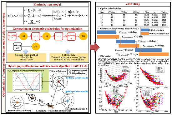
Figure 1. Research framework.

3. Methodology

This section presents the description of the optimization model of construction duration and schedule robustness. In addition, the methodologies of robustness criteria, generation of alternative schedules for optimization, and the proposed HGWOSCA are introduced.

3.1. Problem Formulation

The optimization model of construction duration and schedule robustness is expressed as follows:

$$\{\begin{array}{l}Opt(r_s,r_p,T)\\ r_s={\displaystyle \sum _{i=0}^n{w}_i}(\left|S_i-s_i\right|)\\ r_p={\displaystyle \sum _{i=0}^n{w}_i}(\left|P_i-p_i\right|)\\ T={\displaystyle \sum _{i\in \mathrm{critical}\mathrm{path}}^{}(SB+T(i))}+PB\end{array}$$

(1)

subject to:

$$\{\begin{array}{l}\max \left[s_{i-1}+T(i-1)\right]\le S_i,i\ge 1\\ \max \left[s_{i-1}+T(i-1)+SB+FB\right]\le S_i,i\ge 1\\ {\displaystyle \sum r}\le R\end{array}$$

(2)

where, three optimization objectives are proposed. r_s is the robustness criterion proposed from the aspect of deviation of an activity’s starting time, r_p is the robustness criterion proposed from the aspect of logical relationships among activities, and T represents the total construction duration of the schedule. The detailed descriptions of the symbols in this paper are shown in Appendix A.

3.2. Robustness Criteria

Robustness criteria are the foundation for the optimization model. Since activities and logical relationships among activities are two indispensable components of a construction schedule [6], two criteria (i.e., starting time deviation (r_s) and structural deviation (r_p)), are proposed to measure the schedule robustness from these two aspects. r_s is the robustness criterion proposed from the aspect of activities’ starting time, and r_p is the robustness criterion proposed from the aspect of logical relationships among activities. These two criteria provide a more comprehensive understanding of measuring schedule robustness.

The starting time deviation r_s is the absolute value of the weighted summation of the deviations between the starting times of the actual activities and the planned activities.

$$r_s={\displaystyle \sum _{i=0}^n{w}_i}(\left|S_i-s_i\right|).$$

(3)

The structural deviation r_p is the absolute value of the weighted summation of the deviations between the orders of the actual activity and the planned activity.

$$r_p={\displaystyle \sum _{i=0}^n{w}_i}(\left|P_i-p_i\right|).$$

(4)

As seen from the above equations, the smaller the r_s and r_p values, the better the robustness.

3.3. Generation of Alternative Schedules for Optimization

With the robustness criteria as the optimization objectives, the next step was to improve schedule robustness to generate alternative schedules for optimization. This included two parts (as shown in Figure 2): Identifying the critical chain in the schedule by critical chain method and allocating buffers to it by using the STC method.

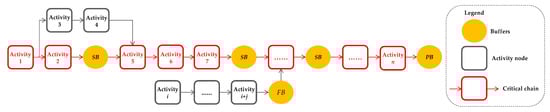
Figure 2. Generation of alternative schedules with buffers allocated based on critical chain method and the starting time criticality (STC) method.

The critical chain is a chain composed of activities that are interdependent due to time conflicts and resource conflicts. Since the constraints which exist in each schedule correspond to the bottleneck elements that prevent the project from being completed on schedule [7], it is effective to identify the conflicting activities so as to improve the schedule robustness.

The identification process of a critical chain was as follows:

• Compute the initial schedule via simulation.
• Identify the activities that can be postponed on the condition that the schedule fulfils the resource constraints and logical relationships. An activity which cannot be postponed was denoted as NonAi; otherwise, it was denoted as MovAi. A MovAi which does not satisfy the resource constraints was denoted as NonBi; otherwise, it was denoted as MovBi.
• The critical chain was identified by combining NonAi and NonBi. If there was more than one critical chain, the chain with the most activities was selected as the final critical chain, and the others were treated as non-critical chains.

After the critical chain was identified, three types of buffers, including project buffer (PB), scattered buffer (SB), and feeding buffer (FB), were allocated to it. PB was allocated at the end of the critical chain to ensure the project was completed on time. SBs were allocated in front of highly critical activities to ensure that these activities started on schedule. FBs were allocated where non-critical chains feed into the critical chain in order to prevent a delay of the activity on the critical chain when the activities on the non-critical chain were delayed.

The sizes of FB and the sum of PB and SB were determined using the elasticity coefficient method which was improved by the Dezert–Smarandache Theory (DSmT) [54,55].

In the elasticity coefficient method, the (a, b, c) in the three-point estimation method is replaced by (a, b) and c is considered in the elasticity coefficient: $K=(c-a)/(b-a)$. In this way, the impacts of interference factors on schedule can be reflected in buffers. The closer c approaches a, the less likely it is to delay the activity and the smaller the K value. The closer c approaches b, the more likely it is to delay the activity and the greater the K value. Therefore, the buffers can be calculated through K.

$$FB={\displaystyle \sum _{c\in B}\left\{(b^c-a^c)\times K_B^c\right\}},$$

(5)

where B denotes the set of activities related to the buffers.

Additionally, in the elasticity coefficient method, a is the activity duration without considering the impacts of interference factors and is calculated by simulation. The activity durations are represented by b and c and consider varying degrees of impacts of interference factors and are calculated as:

$$b=a\times (1+\min (m_j({\theta }_1),m_j({\theta }_2),m_j({\theta }_3)));$$

(6)

$$c=a\times (1+{\displaystyle \sum _{n=1}^3{m}_j({\theta }_h)}),$$

(7)

where $m_j({\theta }_h)$ is computed using the DSmT method. Delay, downtime, and breakdown happen during construction as a result of interference factors. Hence, it is reasonable to determine the size of buffers according to the impact of interference on schedule. DSmT recognizes the fusion of occurrence probabilities of interference factors. It reasonably solves the problem of large conflicts among interference factors and achieves the unification of occurrence probabilities and impacts of interference factors on schedule.

Interference factor j (j = 1 – 6) represents the geological factor, technical factor, environmental factor, management factor, material factor, and the mechanical factor, respectively. The construction parameter k (k = 1 – 11) represents surveying setting out, charge explosion, safe disposal, explosion slag cleaning, ventilation, disposal of unfavorable geology, other downtime, hand drill, three arm trolley, dump truck and loader, and the consequence of interference factors, respectively. Factor h (h = 1 – 3), represents delay, downtime, and breakdown, respectively. Factor $m_j({\theta }_h)$ is defined as:

$$\{\begin{array}{l}{m}_j({\theta }_1)=m_{{}_j}({\gamma }_1)\oplus \mathrm{...}\oplus m_{{}_j}({\gamma }_6)\\ m_j({\theta }_2)=m_{{}_j}({\gamma }_7)\oplus \mathrm{...}\oplus m_j({\gamma }_9)\\ m_j({\theta }_3)=m_{{}_j}({\gamma }_{10})\oplus m_j({\gamma }_{11})\end{array};$$

(8)

$$\forall A\ne \varnothing \in D^U,\left[m_1+m_2\right](A)={\displaystyle \sum _{{\theta }_1,{\theta }_2\in D^U,{\theta }_1\cap {\theta }_2=A}{m}_1({\theta }_1)m_2({\theta }_2)}.$$

(9)

Then, the STC method and golden section rule were used to determine the locations of scattered buffers. The process is as follows:

• The STC method was adopted to measure the necessity of allocating the buffer before an activity.

  $$\mathrm{stc}(i)=\frac{1}{3}{\displaystyle \sum _{n=1}^3{m}_j({\theta }_h)}\times w_i,$$

  (10)

  where $\frac{1}{3}{\displaystyle \sum _{n=1}^3{m}_j({\theta }_h)}$ denotes the possibility that the activity i does not start on schedule.
• Based on the golden section rule, 38.2% of the buffers that need to be allocated on critical chain were allocated at the end of the critical chain as the project buffer. Based on this same rule, 61.8% of the buffers that need to be allocated on critical chain were allocated in front of activities as the scattered buffers.

  $$PB=0.382{\displaystyle \sum _{c\in B}\left\{(b^c-a^c)\times K_B^c\right\}}.$$

  (11)

  $$SB=0.618{\displaystyle \sum _{c\in B}\left\{(b^c-a^c)\times K_B^c\right\}}.$$

  (12)
• Sort the activities on critical chain from high to low in order of criticality. Add their buffers one by one.
• Judge whether the sum has reached 61.8% of the buffers. It not, go back to step 3.
• If the sum has reached 61.8% of the buffers, the added activities are the activities that scattered buffers are allocated before.

3.4. Optimization of Construction Duration and Schedule Robustness Based on HGWOSCA

In this section, a hybrid multi-objective grey wolf optimizer with sine cosine algorithm is applied to solve the optimization model. The movement directions and speed of GWO was improved by SCA. Then the validity and superiority of the HGWOSCA was demonstrated by comparison with four other algorithms. The solution flow of HGWOSCA for T-r_s-r_p optimization model is presented.

3.4.1. Theory of HGWOSCA

The HGWOSCA contains three phases: Encircling, hunting behavior improved by SCA, and modified searching and attacking behavior. Four types of grey wolves named alpha (α), beta (β), delta (δ), and omega (ω) were employed for mathematically modeling their social hierarchy. The first three fittest solutions are α, β, and δ, respectively. The rest of the candidate solutions are ω. In GWO, the optimization is guided by α, β, and δ, and the ω wolves follow these three.

The encircling behavior is simulated by the following equations:

$$\overrightarrow{D}=\left|\overrightarrow{C}\cdot \overrightarrow{X_p}(t)-\overrightarrow{X}(t)\right|,$$

(13)

$$\overrightarrow{X}(t+1)={\overrightarrow{X}}_p(t)-\overrightarrow{A}\overrightarrow{\cdot D},$$

(14)

where t represents the current iteration, $\overrightarrow{X_p}$ is the position vector of the prey, and $\overrightarrow{X}$ represents the position vector of a grey wolf, $\overrightarrow{A}$ and $\overrightarrow{C}$ are coefficient vectors, which are calculated as follows:

$$\overrightarrow{A}=2\overrightarrow{a}\cdot \overrightarrow{r_1}-\overrightarrow{a},$$

(15)

$$\overrightarrow{C}=2\cdot \overrightarrow{r_2},$$

(16)

where r₁, r₂ are random vectors in [0, 1].

The hunting behavior is simulated by the following equations:

$$\{\begin{array}{l}\overrightarrow{D_{\alpha }}=\left|\overrightarrow{C_1}\cdot \overrightarrow{X_{\alpha }}-\overrightarrow{X}\right|\\ \overrightarrow{D_{\beta }}=\left|\overrightarrow{C_2}\cdot \overrightarrow{X_{\beta }}-\overrightarrow{X}\right|\\ \overrightarrow{D_{\delta }}=\left|\overrightarrow{C_3}\cdot \overrightarrow{X_{\delta }}-\overrightarrow{X}\right|\end{array},$$

(17)

$$\{\begin{array}{l}\overrightarrow{X_1}=\overrightarrow{X_{\alpha }}-\overrightarrow{A_1}\cdot (\overrightarrow{D_{\alpha }})\\ \overrightarrow{X_2}=\overrightarrow{X_{\beta }}-\overrightarrow{A_2}\cdot (\overrightarrow{D_{\beta }})\\ \overrightarrow{X_3}=\overrightarrow{X_{\delta }}-\overrightarrow{A_3}\cdot (\overrightarrow{D_{\delta }})\end{array},$$

(18)

$$\overrightarrow{X}(t+1)=\frac{\overrightarrow{X_1}+\overrightarrow{X_2}+\overrightarrow{X_3}}{3}.$$

(19)

GWO was originally developed for solving continuous optimization problems and cannot be used to solve the combinatorial optimization problems in this paper. Thus, the search operator was modified as follows:

$$\overrightarrow{X}(t+1)=\{\begin{array}{l}shift(\overrightarrow{X}(t),{\overrightarrow{X}}_{\alpha }-\overrightarrow{X}(t)),ifr<\frac{1}{3}\\ shift(\overrightarrow{X}(t),{\overrightarrow{X}}_{\beta }-\overrightarrow{X}(t)),if\frac{1}{3}\le r<\frac{2}{3}\\ shift(\overrightarrow{X}(t),{\overrightarrow{X}}_{\delta }-\overrightarrow{X}(t)),otherwise\end{array}.$$

(20)

If the units were beyond the boundary range, the boundary element was connected to it in the other direction.

The position of α is determined by the position updating equation of SCA [40], by which the position, speed, and convergence accuracy of the grey wolf agent are improved and the convergence performance of GWO is extended.

$$X_l^{t+1}=\{\begin{array}{l}{X}_l^t+r_1\times \sin (r_2)\times \left|r_3{P}_l^t-X_l^t\right|,r_4<0.5\\ X_l^t+r_1\times \cos (r_2)\times \left|r_3{P}_l^t-X_l^t\right|,r_4\ge 0.5\end{array},$$

(21)

where, r₁, r_2, and r₃ are random numbers, and r₄ is a random number used for exploitation and exploration.

3.4.2. Performance of the Proposed HGWOSCA

The efficiency of the proposed HGWOSCA was tested via the patterson_pat1 and patterson_pat20 in the well-known PSPLIB data set [56], as shown in Figure 3. Multi-objective particle swarm optimization (MOPSO), multi-objective grey wolf optimizer (MOGWO), multi-objective evolutionary algorithm (MOEA), and multi-objective multi-verse optimization (MOMVO) were selected for comparison with the HGWOSCA. The tests were implemented on a computer with Intel Core i5, 2.39 GHz, 131,072 MB RAM, with a Windows 10 operating system.

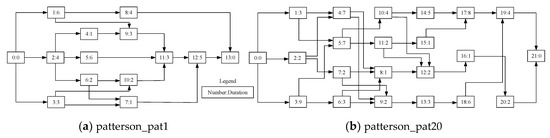
Figure 3. Network of patterson_pat1 and patterson_pat20 [56].

Four metrics including generational distance (GD), inverse generational distance (IGD), ratio of non-dominated individual (RNI), and Spread were employed.

(1) GD represents the distance between the Pareto front and the optimal Pareto front and is formulated as:

$$\mathrm{GD}=\frac{\sqrt{{\displaystyle \sum \begin{array}{l}\left|PF\right|\\ i=1\end{array}}{d}_p^2}}{\left|PF\right|},$$

(22)

where PF is the number of solutions in the Pareto front. The lower the GD value, the better the convergence performance of an algorithm.

(2) IGD represents the distances between each solution in optimal Pareto front and is formulated as:

$$\mathrm{IGD}=\frac{\sqrt{{\displaystyle \sum \begin{array}{l}\\ x\in OPF\end{array}}{d}_p^2}}{\left|OPF\right|},$$

(23)

where OPF is the number of solutions in optimal Pareto front. The lower the IGD value, the better the convergence performance of an algorithm.

(3) RNI represents the ratio of the number of non-dominated individuals to the size of the population and is formulated as:

$$\mathrm{RNI}=\frac{N_{non}}{N}\times 100\%,$$

(24)

where N_non is the number of non-dominated individuals and N is the number of all individuals. The higher the RNI value, the better the solution quality.

(4) Spread represents the extent of spread achieved among the front and is formulated as:

$$\mathrm{Spread}=\frac{{\displaystyle \sum \begin{array}{l}{n}_0\\ q=1\end{array}}{d}_q^e+{\displaystyle \sum \begin{array}{l}\left|PF\right|\\ p=1\end{array}}\left|d_p-\overline{d}\right|}{{\displaystyle \sum \begin{array}{l}{n}_0\\ q=1\end{array}}{d}_q^e+\left|PF\right|\cdot \overline{d}},$$

(25)

where n₀ is the number of objectives. The lower the spread value, the better the distribution of solutions.

Figure 4 and Figure 5 show the four metrics on the algorithms mentioned above over 50 runs. The GD value, IGD value, and spread value of HGWOSCA were the lowest among the five algorithms, and the RNI value of HGWOSCA was the highest among the five algorithms. This result indicates the good performance of the proposed HGWOSCA. Thus, the HGWOSCA is a good fit for multi-objective optimization.

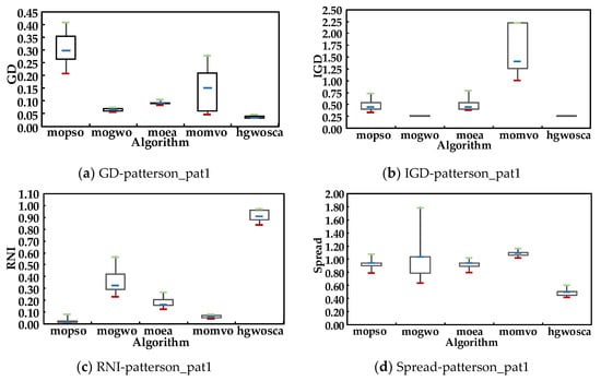
Figure 4. Metrics value of patterson_pat1.

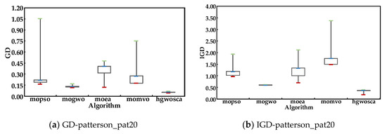
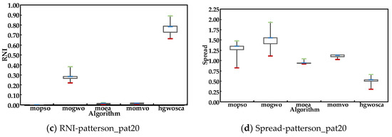
Figure 5. Metrics value of patterson_pat20.

3.4.3. Solution Flow of HGWOSCA for T-r_s-r_p Optimization Model

The proposed HGWOSCA was applied to solve the optimization model of construction duration T, starting time deviation r_s, and structural deviation r_p. A basic flowchart of this is shown in Figure 6.

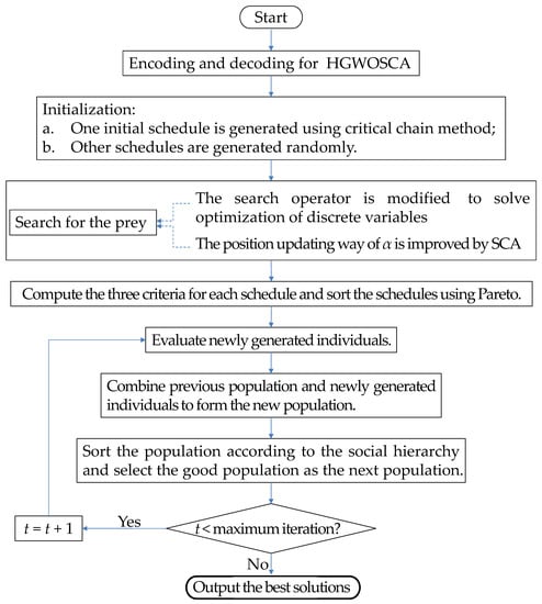
Figure 6. A flowchart of the hybrid grey wolf optimizer with sine cosine algorithm (HGWOSCA).

(1)

Encode the schedule.

(2)

Initialization: To ensure a good diversity of solutions, one schedule was generated using the method proposed in Section 3.3 and other schedules were generated randomly.

(3)

Search for the prey. The search operator of GWO was originally developed to solve continuous optimization problems [57], which was not suitable to solve the optimization problems of discrete variables. Thus, in this paper, the search operator was modified as shown in Section 3.4.1. Secondly, the position updating way of α was improved by SCA to improve the searching capability of GWO as shown in Section 3.4.1.

(4)

Compute the three criteria for each schedule and sort the schedules using Pareto relationship. According to the Pareto dominance nature of multi-objective optimization problems, there is no unique optimal solution but a set of non-dominated solutions. Thus, the population can be divided into several ranks according to the Pareto dominance relationship. The solutions at the first level rank are denoted as α solutions, the solutions at the second level rank are denoted as β solutions, the solutions at the third level rank are denoted as δ solutions, and the other solutions are donated as ω solutions.

(5)

Evaluate: The newly generated individuals were evaluated based on the fitness values. The best individuals were saved and combined with the previous population to form the new population. Then the populations were sorted according to the social hierarchy and the good population was selected as the new population.

(6)

Judgment: Determine whether the algorithm satisfies the termination condition. If yes, output the best solutions; otherwise, let t = t+1 and go back to step 5.

(7)

Output: Output the best solutions which are the schedules with both short construction duration and good schedule robustness.

4. Case Study

A real-life underground power station in Southwest China was selected as a case study to demonstrate the rationality of the research in this paper. The layout of the underground power station is shown in Figure 7. It is composed of a main workshop, main transformer, last chamber, and several branch tunnels.

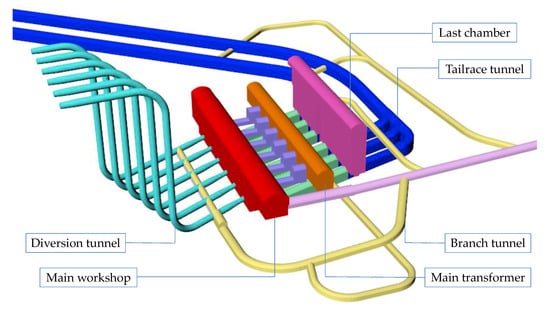
Figure 7. Layout of the project.

According to the construction arrangement provided by the design institute, the initial schedule’s information was: T = 2376 days, r_s = 82.66 days, and r_p = 0.98. Then, the optimized schedules were obtained after 200 iterations of optimization. Five of them are shown in Table 1. These schedules had better performance for both construction duration and schedule robustness. The optimized schedules corresponded to a set of Pareto optimal solutions rather than a unique solution. This is because a conflict exists between construction duration and schedule robustness, and they cannot be directly compared. It is impossible to improve either objective without weakening the others. Therefore, the optimized schedules in Table 1 met the requirements of multiple objectives and provided a variety of satisfying schedules. Gantt chart of main workshop layer #1–#4 of the optimized schedule No. 1 in Table 1 is shown in Figure 8 as a detailed presentation, in which the duration of each activity and the schedule of robustness is clearly shown.

Table 1. Optimized schedule.

Schedule Number	PB/day	FB/day	SB/day	rs/day	rp	T/day
1	19	22	14	75.12	0.6027	2398
2	19	22	6	76.13	0.6072	2393
3	19	22	30	75.05	0.6027	2401
4	20	22	12	75.28	0.6126	2396
5	20	22	23	75.07	0.6027	2399

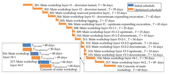
Figure 8. Gantt chart of the main workshop layer #1–#4 of the optimized schedule No. 1.

5. Discussion

To determine the effectiveness of the proposed HGWOSCA for optimization of construction duration and schedule robustness, four algorithms including MOPSO, MOGWO, MOEA, and MOMVO were selected for comparison. To make a fair comparison among these algorithms, the same encoding scheme and initialization were used as HGWOSCA. Each algorithm ran 500 iterations independently and the maximum number of solutions was set as 200.

The Pareto front obtained by the five algorithms above is shown in Figure 9, in which (a) provides a three-dimensional view with r_s, r_p, and T; (b) provides a two-dimensional view with r_s and T; (c) provides a two-dimensional view with r_p and T; and (d) provides a two-dimensional view with r_s and r_p. It can be seen that the HGWOSCA can approach closer to the Pareto front than the other algorithms, which implies that the HGWOSCA can obtain better solutions than the other four algorithms. The proposed HGWOSCA is therefore superior to its compared algorithms for optimization of construction duration and schedule robustness.

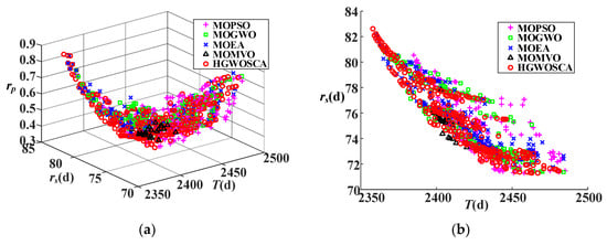
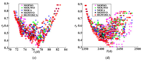
Figure 9. Pareto fronts (PF) obtained by different algorithms under different angles: (a) PF with r_s, r_p and T; (b) PF with r_s and T; (c) PF with r_s and r_p; (d) PF with r_s and T.

The four metrics of HGWOSCA and the other four algorithms used for comparison are shown in Table 2. The GD value of HGWOSCA was the lowest, which indicates that HGWOSCA had a better convergence performance. The IGD value of HGWOSCA was the lowest, which indicates that HGWOSCA had the better diversity and convergence performance. The RNI value of HGWOSCA was the highest, which indicates that HGWOSCA had the better accuracy performance. The spread value of HGWOSCA was the lowest, which indicates that HGWOSCA had the better distribution performance. Therefore, HGWOSCA is superior in its performance of convergence, diversity, accuracy, and distribution for optimization of construction duration and schedule robustness.

Table 2. Four metrics based on different algorithms.

	Algorithm	MOPSO	MOGWO	MOMVO	MOEA	HGWOSCA
Metric
GD		0.0636	0.0518	0.1599	0.0529	0.0500
IGD		2.9819	0.8866	16.361	0.9196	0.7176
RNI		0.2079	0.0528	0.0792	0.0660	0.597
Spread		0.7186	0.7164	0.9680	0.8096	0.6984

6. Conclusions

Construction duration and schedule robustness have great significance in construction schedule management. However, most related researches which take both construction duration and schedule robustness into account only considered schedule robustness via starting time deviation. Additionally, a more efficient algorithm is worth being developed to solve the optimization model. To overcome these limitations, an optimization model of construction duration and schedule robustness was proposed, which considered starting time deviation and structural deviation. An underground power station in China was used for a case study to verify its applicability and advantages. The major contributions are summarized as follows:

• Considering schedule robustness via starting time deviation and structural deviation, a novel optimization model of construction duration and schedule robustness was proposed.
• Alternative schedules were generated using critical chain method and STC method to allocate buffers centrally and scatteredly.
• The hybrid grey wolf optimizer with sine cosine algorithm (HGWOSCA) was developed to solve the optimization model.

Overall, the proposed optimization model of construction duration and schedule robustness is applicable and has practical significance for multi-objective construction schedule management. In future research, an optimization system version centered on human–computer interaction can be generated to improve solving efficiency and operability for optimization.

References

- Clemente-Císcar, M.; San Matías, S.; Giner-Bosch, V. A methodology based on profitability criteria for defining the partial defection of customers in non-contractual settings. Eur. J. Oper. Res. 2014, 239, 276–285. [Google Scholar] [CrossRef]
- Kobylański, P.; Kuchta, D. A note on the paper by M. A. Al-Fawzan and M. Haouari about a bi-objective problem for robust resource-constrained project scheduling. Int. J. Prod. Econ. 2007, 107, 496–501. [Google Scholar] [CrossRef]
- Van de Vonder, S.; Ballestín, F.; Demeulemeester, E.; Herroelen, W. Heuristic procedures for reactive project scheduling. Comput. Ind. Eng. 2007, 52, 11–28. [Google Scholar] [CrossRef]
- Lambrechts, O.; Demeulemeester, E.; Herroelen, W. A tabu search procedure for developing robust predictive project schedules. Int. J. Prod. Econ. 2008, 111, 493–508. [Google Scholar] [CrossRef]
- Ning, M.; He, Z.; Jia, T.; Wang, N. Metaheuristics for multi-mode cash flow balanced project scheduling with stochastic duration of activities. Autom. Constr. 2017, 81, 224–233. [Google Scholar] [CrossRef]
- Zhong, D.H.; Bi, L.; Yu, J.; Zhao, M.Q. Robustness analysis of underground powerhouse construction simulation based on Markov Chain Monte Carlo method. Sci. China Technol. Sci. 2016, 59, 252–264. [Google Scholar] [CrossRef]
- Eliyahu, M.G. Critical Chain, 1st ed.; The North River Press: Great Barrington, MA, USA, 1997. [Google Scholar]
- Hu, X.; Cui, N.; Demeulemeester, E.; Bie, L. Incorporation of activity sensitivity measures into buffer management to manage project schedule risk. Eur. J. Oper. Res. 2016, 249, 717–727. [Google Scholar] [CrossRef]
- Hu, X.; Demeulemeester, E.; Cui, N.; Wang, J.; Tian, W. Improved critical chain buffer management framework considering resource costs and schedule stability. Flex. Serv. Manuf. J. 2017, 29, 159–183. [Google Scholar] [CrossRef]
- Tian, M.; Liu, R.J.; Zhang, G.J. Solving the resource-constrained multi-project scheduling problem with an improved critical chain method. J. Oper. Res. Soc. 2019, 1–16. [Google Scholar] [CrossRef]
- Shurrab, M. Traditional Critical Path Method versus Critical Chain Project Management: A Comparative View. Int. J. Econ. Manag. Sci. 2015, 4, 4–9. [Google Scholar] [CrossRef]
- Montazeri, B. Comparing Critical Chain Project Managemenet with Critical Path Method: A Case Study. Master’s Thesis, Western Kentucky University, Bowling Green, KY, USA, 2017. [Google Scholar]
- Sarkar, D.; Jha, K.N.; Patel, S. Critical chain project management for a highway construction project with a focus on theory of constraints. Int. J. Constr. Manag. 2018, 1–14. [Google Scholar] [CrossRef]
- Ke, H.; Wang, L.; Huang, H. An uncertain model for RCPSP with solution robustness focusing on logistics project schedule. Int. J. E Navigation Marit. Econ. 2015, 3, 71–83. [Google Scholar] [CrossRef]
- Bruni, M.E.; Di Puglia Pugliese, L.; Beraldi, P.; Guerriero, F. An adjustable robust optimization model for the resource-constrained project scheduling problem with uncertain activity durations. Omega UK 2017, 71, 66–84. [Google Scholar] [CrossRef]
- Ghoddousi, P.; Ansari, R.; Makui, A. An improved robust buffer allocation method for the project scheduling problem. Eng. Optim. 2017, 49, 718–731. [Google Scholar] [CrossRef]
- Lambrechts, O.; Demeulemeester, E.; Herroelen, W. Time slack-based techniques for robust project scheduling subject to resource uncertainty. Ann. Oper. Res. 2011, 186, 443–464. [Google Scholar] [CrossRef]
- Ning, Y.; Peng, Z.; Dai, Y.; Bi, D.; Wang, J. Enhanced particle swarm optimization with multi-swarm and multi-velocity for optimizing high-dimensional problems. Appl. Intell. 2019, 49, 335–351. [Google Scholar] [CrossRef]
- Oliveira, R.; Figueiredo, A.; Vicente, R.; Almeida, R.M.S.F. Multi-objective optimisation of the energy performance of lightweight constructions combining evolutionary algorithms and life cycle cost. Energies 2018, 11, 1683. [Google Scholar] [CrossRef]
- Yıldız, A.; Yıldız, B.; Sait, S.; Li, X. The Harris hawks, grasshopper and multi-verse optimization algorithms for the selection of optimal machining parameters in manufacturing operations. Mater. Test. 2019, 61, 725–733. [Google Scholar] [CrossRef]
- Zhang, L.; Gao, Y.; Sun, Y.; Fei, T.; Wang, Y. Application on Cold Chain Logistics Routing Optimization Based on Improved Genetic Algorithm. Autom. Control. Comput. Sci. 2019, 53, 169–180. [Google Scholar] [CrossRef]
- Wu, L.; He, Z.; Chen, Y.; Wu, D.; Cui, J. Brainstorming-Based Ant Colony Optimization for Vehicle Routing with Soft Time Windows. IEEE Access 2019, 7, 19643–19652. [Google Scholar] [CrossRef]
- Zhang, J.; Zhong, D.; Zhao, M.; Yu, J.; Lv, F. An optimization model for construction stage and zone plans of rockfill dams based on the enhanced whale optimization algorithm. Energies 2019, 12, 466. [Google Scholar] [CrossRef]
- Faris, H.; Aljarah, I.; Al-Betar, M.A.; Mirjalili, S. Grey wolf optimizer: A review of recent variants and applications. Neural Comput. Appl. 2018, 30, 413–435. [Google Scholar] [CrossRef]
- Yang, Z.; Liu, C. A hybrid multi-objective gray wolf optimization algorithm for a fuzzy blocking flow shop scheduling problem. Adv. Mech. Eng. 2018, 10. [Google Scholar] [CrossRef]
- Jiang, T.; Zhang, C.; Zhu, H.; Deng, G. Energy-efficient scheduling for a job shop using grey wolf optimization algorithm with double-searching mode. Math. Probl. Eng. 2018, 2018, 1–12. [Google Scholar] [CrossRef]
- Jiang, T. A Hybrid Grey Wolf Optimization for Job Shop Scheduling Problem. Int. J. Comput. Intell. Appl. 2018, 17, 1–12. [Google Scholar] [CrossRef]
- Long, W.; Liang, X.; Cai, S.; Jiao, J.; Zhang, W. A modified augmented Lagrangian with improved grey wolf optimization to constrained optimization problems. Neural Comput. Appl. 2017, 28, 421–438. [Google Scholar] [CrossRef]
- Kohli, M.; Arora, S. Chaotic grey wolf optimization algorithm for constrained optimization problems. J. Comput. Des. Eng. 2018, 5, 458–472. [Google Scholar] [CrossRef]
- Luo, K. Enhanced grey wolf optimizer with a model for dynamically estimating the location of the prey. Appl. Soft Comput. J. 2019, 77, 225–235. [Google Scholar] [CrossRef]
- Ren, Y.; Ye, T.; Huang, M.; Feng, S. Gray Wolf Optimization algorithm for multi-constraints second-order stochastic dominance portfolio optimization. Algorithms 2018, 11, 72. [Google Scholar] [CrossRef]
- Long, W.; Jiao, J.; Liang, X.; Tang, M. Inspired grey wolf optimizer for solving large-scale function optimization problems. Appl. Math. Model. 2018, 60, 112–126. [Google Scholar] [CrossRef]
- Li, M.Q.; Xu, L.P.; Xu, N.; Huang, T.; Yan, B. SAR image segmentation based on improved grey wolf optimization algorithm and fuzzy c-means. Math. Probl. Eng. 2018, 2018, 1–11. [Google Scholar] [CrossRef]
- Yu, S.; Lu, H. An integrated model of water resources optimization allocation based on projection pursuit model—Grey wolf optimization method in a transboundary river basin. J. Hydrol. 2018, 559, 156–165. [Google Scholar] [CrossRef]
- Maroufpoor, S.; Maroufpoor, E.; Bozorg-Haddad, O.; Shiri, J.; Mundher Yaseen, Z. Soil moisture simulation using hybrid artificial intelligent model: Hybridization of adaptive neuro fuzzy inference system with grey wolf optimizer algorithm. J. Hydrol. 2019, 575, 544–556. [Google Scholar] [CrossRef]
- Zou, Q.; Liao, L.; Ding, Y.; Qin, H. Flood classification based on a fuzzy clustering iteration model with combined weight and an immune grey wolf optimizer algorithm. Water 2019, 11, 80. [Google Scholar] [CrossRef]
- Majumdar, K.; Das, P.; Roy, P.K.; Banerjee, S. Solving OPF Problems using Biogeography Based and Grey Wolf Optimization Techniques. Int. J. Energy Optim. Eng. 2017, 6, 55–77. [Google Scholar] [CrossRef]
- Dai, S.; Niu, D.; Li, Y. Daily peak load forecasting based on complete ensemble empirical mode decomposition with adaptive noise and support vector machine optimized by modified grey Wolf optimization algorithm. Energies 2018, 11, 163. [Google Scholar] [CrossRef]
- Singh, D.; Dhillon, J.S. Ameliorated grey wolf optimization for economic load dispatch problem. Energy 2019, 169, 398–419. [Google Scholar] [CrossRef]
- Mirjalili, S. SCA: A Sine Cosine Algorithm for solving optimization problems. Knowl. Based Syst. 2016, 96, 120–133. [Google Scholar] [CrossRef]
- Rizk-Allah, R.M. Hybridizing sine cosine algorithm with multi-orthogonal search strategy for engineering design problems. J. Comput. Des. Eng. 2018, 5, 249–273. [Google Scholar] [CrossRef]
- Gupta, S.; Deep, K. A hybrid self-adaptive sine cosine algorithm with opposition based learning. Expert Syst. Appl. 2019, 119, 210–230. [Google Scholar] [CrossRef]
- Ekinci, S. Optimal design of power system stabilizer using sine cosine algorithm. J. Fac. Eng. Archit. Gazi Univ. 2019, 34, 1329–1350. [Google Scholar]
- Das, S.; Bhattacharya, A.; Chakraborty, A.K. Solution of short-term hydrothermal scheduling using sine cosine algorithm. Soft Comput. 2018, 22, 6409–6427. [Google Scholar] [CrossRef]
- Issa, M.; Hassanien, A.E.; Oliva, D.; Helmi, A.; Ziedan, I.; Alzohairy, A. ASCA-PSO: Adaptive sine cosine optimization algorithm integrated with particle swarm for pairwise local sequence alignment. Expert Syst. Appl. 2018, 99, 56–70. [Google Scholar] [CrossRef]
- Li, S.; Fang, H.; Liu, X. Parameter optimization of support vector regression based on sine cosine algorithm. Expert Syst. Appl. 2018, 91, 63–77. [Google Scholar] [CrossRef]
- Hekimoğlu, B. Sine-cosine algorithm-based optimization for automatic voltage regulator system. Trans. Inst. Meas. Control 2019, 41, 1761–1771. [Google Scholar] [CrossRef]
- Elaziz, M.A.; Hemedan, A.A.; Ostaszweski, M.; Schneider, R.; Lu, S. Optimization ACE inhibition activity in hypertension based on random vector functional link and sine-cosine algorithm. Chemom. Intell. Lab. Syst. 2019, 190, 69–77. [Google Scholar] [CrossRef]
- Tasnin, W.; Saikia, L.C. Maiden application of an sine-cosine algorithm optimised FO cascade controller in automatic generation control of multi-area thermal system incorporating dish-Stirling solar and geothermal power plants. IET Renew. Power Gener. 2018, 12, 585–597. [Google Scholar] [CrossRef]
- Wang, J.; Yang, W.; Du, P.; Niu, T. A novel hybrid forecasting system of wind speed based on a newly developed multi-objective sine cosine algorithm. Energy Convers. Manag. 2018, 163, 134–150. [Google Scholar] [CrossRef]
- Liu, S.; Feng, Z.K.; Niu, W. jing; Zhang, H. rong; Song, Z.G. Peak operation problem solving for hydropower reservoirs by elite-guide sine cosine algorithm with Gaussian local search and random mutation. Energies 2019, 12, 2189. [Google Scholar] [CrossRef]
- Fu, W.; Wang, K.; Li, C.; Li, X.; Li, Y.; Zhong, H. Vibration trend measurement for a hydropower generator based on optimal variational mode decomposition and an LSSVM improved with chaotic sine cosine algorithm optimization. Meas. Sci. Technol. 2019, 30. [Google Scholar] [CrossRef]
- Xu, K.K.; Li, H.X.; Yang, H.D. Kernel-based random vector functional-link network for fast learning of spatiotemporal dynamic processes. IEEE Trans. Syst. Man Cybern. Syst. 2017, 99, 1–11. [Google Scholar] [CrossRef]
- Smarandache, F.; Dezert, J. Advances and Applications of DSmT for Information Fusion (Collected Works); American Research Press: Rehoboth, DE, USA, 2015. [Google Scholar]
- Code for the Buffer Size Determination. Available online: http://martin.iutlan.univ-rennes1.fr/Doc/GeneralBeliefFunctionsFramework.tar (accessed on 1 January 2015).
- Kolisch, R.; Sprecher, A. PSPLIB—A project scheduling problem library. Eur. J. Oper. Res. 1997, 96, 205–216. [Google Scholar] [CrossRef]
- Mirjalili, S.; Mirjalili, S.M.; Lewis, A. Grey Wolf Optimizer. Adv. Eng. Softw. 2014, 69, 46–61. [Google Scholar] [CrossRef]
© 2020 by the authors. Licensee MDPI, Basel, Switzerland. This article is an open access article distributed under the terms and conditions of the Creative Commons Attribution (CC BY) license (http://creativecommons.org/licenses/by/4.0/).