Low-Frequency Wind Energy Variability in the Continental Contiguous United States

Abstract

Wind energy is characterized by exceptionally large power fluctuations at the single energy facility level, that remain significant also considering the average of the many different energy facilities connected to the same grid. A high-frequency statistic, 1 min or less sampling time, is needed to understand this variability and design the energy storage facilities needed to replace the combustion fuel power plants now used to stabilize a grid. While high-frequency data are unavailable for the United States, low-frequency data, collected monthly, allow assessing the month-to-month and year-to-year variability, and define a low-frequency variability “performance”. The manuscript analyzes the output of the onshore wind energy facilities of capacity more than 250 MW in the continental contiguous United States. The differences between wind energy facilities within the same macro-region, also in about the same location, are shown, for both the annual average capacity factor and the low-frequency variability parameters. Wind energy facilities with larger annual average capacity factors have reduced variability parameters, both seasonal and inter-annual, thus performing better. The facilities with a larger annual average capacity factor also feature smaller variations in between their monthly and annual outputs.

1. Introduction

Information about the contribution of wind energy to the “global energy mix” may be found in [1,2,3,4]. The renewable energy contribution to the global energy mix is growing steadily. If hydroelectric and waste biomass is excluded, the wind is the major contributor, followed by solar photovoltaics. However, the contribution by traditional energy sources especially combustion fuels remains overwhelming [1,4]. According to the International Energy Agency (IEA) [1], the 2016 World Total Primary Energy Supply (TPES) by source was 31.9% oil, 27.1% coal (counting pet and oil shale), 22.1% natural gas, 9.8% waste and biofuels, 4.9% nuclear, 2.5% hydroelectric, and 1.7% all the others, including wind, geothermal, solar, tide, wave, and ocean. Thus, TPES by wind and solar is still small, but it is becoming sizeable, especially for wind, and more recently, solar photovoltaics. As per the IEA [1], the 2016 electricity generation by source was 38.4% coal, 23.2% natural gas, 16.3% hydroelectric, 10.4% nuclear, 3.7% oil, and 8% non-hydro renewable energy and waste, including not only wind, geothermal, solar, tide, wave, and ocean, but also biofuels and waste. Thus, wind and solar start to contribute significantly to electricity needs. Wind energy is providing significant contributions to electricity generation in many countries, the same as solar photovoltaics. Within the United States (US), in 2017 wind energy contributed to 6.3% of the total US utility-scale electricity generation, with a dramatic growth from the 6 billion kWh of the year 2000 to about 254 billion kWh of the year 2017 [2,3].

Wind energy fundamentals are very well known. The amount of power P a wind turbine (WT) can harness from the wind depends on the speed of the wind, WT swept area, and air density, given by

$$P_e=\eta ·\frac{1}{2}·\rho ·A·U^3$$

(1)

In this equation U is the short-term average speed of the wind, ρ is the short-term average air density, A is the WT rotor swept area, and $\eta$ is the total WT efficiency. $\eta$ comprises of the aerodynamic efficiency of the power generation unit (dependent on U), the efficiency of the power transmission, and the efficiency of the electrical generator. WTs achieve peak aerodynamic efficiency of 75–80% of the Betz limit, which is 16/27 (59.3%). Additional losses can be attributed to transmission, while the efficiency of the electric generator is typically remarkably high.

Different WTs provide a different curve for the total WT efficiency $\eta$, Equation (1) [5].

The swept area of the WT is the most relevant design parameter being considered. Higher power output can be achieved by increasing the swept area. Increasing the blade length results in a significant increase in the power available to the WT. Power also increases with hub height. Adaptation to the changing wind direction also improves the wind energy collection.

The mean annual speed of the wind is the most relevant parameter to assess the resource for a wind energy facility (WEF). The wind resource assessment is an essential element to investigate before “siting” in a WEF, as the amount of power in the wind varies with the speed of wind cube, and the wind power density, wind power per unit area, is often used to compare sites. The wind is not constant, but changes in time, in both magnitude and direction, and with the elevation. It is also a function of the specific orography and it also depends on the interaction of the different WTs composing a WEF. The air density is another relevant parameter. Air density varies with pressure, temperature. It changes with time, due to daily and seasonal variations. Additionally, pressure and temperature and thus density also vary with elevation.

The prevailing speed of wind in the direction normal to the WT axis, the prevailing air pressure and temperature, and, to a minor extent, the humidity, and the spatial distribution of all these parameters at the entry of the rotor affect the power output. Non-uniformity of inflow, wake effects of other WTs in an energy facility, turbulence effects, and atmospheric stability effects are discussed in many references.

Power losses and turbulence intensity in WT wakes for offshore installations are reported in [6]. A review of WT wake research is proposed in [7]. WT wake aerodynamics are discussed in [8]. Wind and turbulence laser measurements around large WT are reported in [9]. Lidar and sodar Doppler beam swinging measurements of WT wakes are discussed in [10]. The modeling of WT wakes and WEF are surveyed in [11]. The impact of turbulence intensity and atmospheric stability on power deficits due to WT wakes are discussed in [12]. The wake effect in a large offshore WEF of Denmark is reported in [13,14].

A WEF nameplate capacity is conventionally approximated as the number of WTs by the nominal capacity of each WT [15,16]. However, this is an oversimplification, as the interaction between the WTs may reduce the power output, and the flow conditions over a large area may vary significantly. The amount of land required for a WEF varies depending mostly on the size of the WEF (installed capacity or number and type of WTs), the characteristics of the terrain, prevailing winds, and rotor diameter. These last two particularly determine the WT spacing. WT spaced between 5 and 10 rotor diameters apart is recommended. WT installed 3 or 4 rotor diameters apart when the prevailing winds are from the same direction, or between 5 and 7 rotor diameters when multi-directional wind conditions are often proposed. The power produced at a given prevailing speed of wind in an area may vary from the sum of the power a single WT would produce at that speed.

Computational tools to predict the actual performance of a WEF more accurately in a specific location, including the efficiency penalty by the interference between the WTs of a WEF, are provided in [17]. WAsP (Wind energy industry-standard software) [17] provides wind resources permitting an estimation of power productions from WEF. This analysis tool integrates wind resource and turbulence mapping in complex terrain sites, consisting of the assessment of wind conditions for individual WT in a WEF. Data includes the mean speed of the wind, wind gradient parameters, ambient turbulence, and wind flow inclination.

Wind energy offers advantages, and challenges, in the global energy mix [18,19], with efforts aimed at addressing the challenges to greater use of this energy. Wind-energy is well priced, even if it is not competitive yet with combustion fuels. It is a clean, sustainable energy resource. WEF can be built on existing energy facilities or ranches, even if alternative uses for the land may be more profitable. Good wind energy resources are often available in remote locations, and long transmission lines are needed. WTs cause infrasound noise and visual pollution and damage wildlife. Deforestation for the siting of WEF and transmission lines also creates an environmental impact. The challenge here addressed is the reliability of the wind energy supply, as wind is a fluctuating source of energy translating in a variable supply of electricity to the grid that changes from hour-by-hour, day-by-day, month-by-month, year-by-year, and it is somehow different WEF-by-WEF.

The link between wind energy production and wind energy resource is intuitive. However, other factors affect electricity production. The specific literature for wind energy in the US defines different techno-resource group (TRG) areas [20,21,22,23]. Every area is described by a reference speed of the wind, and reference values of capital expenditures (CAPEX), in $ per unit capacity, and reference capacity factor. The capacity factor ε is defined as the ratio of actual generating power to nominal capacity. It is, therefore, a measure of the power of actual electricity production vs. the theoretically maximum power of electricity production.

What is only partially covered in the literature is the variability of ε on a monthly, annual, and inter-annual basis due to the specific design of the WEF, in about same TRG area (the most part of the WEF here considered are located in TRG 5–7), or even in about the same location (some WEF are located very close to each other, in areas of exactly the same reference speed of wind).

Wind resource variability has been previously analyzed, but mostly with low-frequency (L-F) data. The wind is known for its variability, which is linked to global circulation (geostrophic winds) and local or small-scale circulations such as valley and mountain winds, land and sea breezes, and tunnel effects [24,25]. Geostrophic winds are latitude dependent as they originate from a force generated by a pressure gradient due to non-uniform heating of the atmosphere at different latitudes on the globe. This gradient force is combined with the effect of the Coriolis force, resulting from the latitude and angular rotation of the earth due to a rotating reference frame (earth) [26,27]. Another systematic effect on the speed of the wind is due to friction at the earth’s surface due to the boundary layer (BL). This is the near-earth surface layer of the atmosphere with not negligible viscous forces [28]. This introduces another force on the moving air that slows down the flow [27]. This force decreases with height and becomes negligible above the BL. However, most WTs are operating within the BL region. This effect produces a specific wind gradient profile along with the BL, which is modeled, given a proper estimation of the terrain roughness length. In addition to these systematic effects on the speed of the wind, other large scales (hurricanes, monsoons circulation, and extratropical cyclones) and small-scale (thunderstorm, and tornadoes) effects can change the speed of the wind. More complex global meteorological phenomena are responsible for lower frequency variations of the wind resource [29]. The climate parameters, such as temperature or sea levels, oscillate with inter-annual, decadal, and multi-decadal periodicities (see [30,31,32]). The longest known periodicity is the quasi-60 years’ period.

All these effects together provide a wind variability that is categorized based on the data available as inter-annual, annual, diurnal, and short terms (gusts and turbulence). Inter-annual variability is relevant for inter-annual wind analysis and it takes at least 5 years of data to estimate an average speed of wind at a location. Climate variability usually works over much longer time windows decadal and multi-decadal, with a quasi-60 years’ oscillation clearly evidenced in many parameters.

Unfortunately, there are no wind data spanning more than six decades and even less than that, neither WEF operation data. Prediction models for the inter-annual speed of wind are still sought after as quite complex. The annual wind speed variability is known in most parts of the world where WTs are erected as typically wind speed statistical distribution is found to model the data [25].

Statistical techniques and numerical weather prediction (NWP) models are used to predict the speed of the wind and WT power. The first technique is used for short-term variability or when high spatial resolution is needed. They are applied to a small number of sites. NWP models are methods applied when large-scale integration studies are needed, as they can be used to simulate many locations correlated with local weather phenomena. These methods, however, tend to overestimate wind energy production and underestimate the variability.

Seasonal and inter-annual variability are discussed mostly on a large scale, as outlined below. Specifically, in [33] a global study has been carried out on the inter-annual wind and solar resources variability, with the findings of an average coefficient of variation of 11% for monthly variation between 5 years in the period 1980–2016. The estimated coefficient of variation varies across latitudes, with a peak at high latitudes on land and mid-latitudes on water. Seasonal differences show, in general, rainy seasons have a higher coefficient of variation than dry seasons, the second ones also corresponding to lower wind potentials. In Europe, coefficients of variation were found to with variability in winter as compared to summer, while in South-East Asia the trend is opposite, and in North America is mixed (see below). This approach links variability to global-scale climate and it is only applicable for specific locations inter-annual variability prediction of wind energy production. Similar L-F variability is proposed in [34,35]. When large geographical analysis of wind power is performed the variability of wind energy production is reduced, with an increase of predictability, as shown in [36]. The wind variability should be addressed as the speed of wind changes in space and time about one location, considering the changes in the wind speed and direction, temperature, and barometric pressure, in front of each WT of a WEF installation. By not taking this into account, it can result in an underestimation of energy production variability within years and in a single year, as it is shown in [37].

Studies based on wind energy production variability and thus directly in terms of ε are scarce because large-scale wind energy production has only started to emerge in the last 18 years. Proper evaluation of interannual and seasonal variability of ε should be carried out over 60 years of data to compare the variability with climate models. Most of the current studies are limited in a maximum of 8 years of data. In [37] the hourly energy production of WEF is shown and the statistical distribution of the ε in the Northern Countries (Denmark, Finland, Sweden, and Norway) is reported and compared with the variability of ε of the entire northern region. In this study, the data were limited to the three years from 2000–2002 but the data were hourly ε. Apart from differences in the average ε for each country, with average over the all-region of 25%, it is observed that the standard deviation of a single site (28%) is larger than ε at that site (25%), while by combining more than one site, up to the agglomeration of the Northern countries sites, the final standard deviation is well below the average ε of the order of 15% (the average inter-annual ε is 25%). It must be noted that such a smooth variability in the large area values of ε, in addition to anti-correlated wind energy productions at different plants that are significantly apart from each other (1000 km), it is mainly due to the variability [37] calculated as the variance of the average, which notoriously decreases with the number of data, and it is mostly an artificial effect. The particularly short-time analysis of this study makes the conclusion a little statistically robust. In Central and Northern Europe, the seasonal variability indicates more production in winter than in summer, while the diurnal variability can be appreciated only in Summer, with maximum production occurring between 11:00 and 18:00 h.

In addition to yet not fully understood prediction of inter-annual wind speed variability, a key point remains the estimate of the ε in a specific region. In [38], the analysis of wind power data from four WEF in distinct parts of the US provides a large inter-annual variability, and it has been found that the climate and regional weather patterns are the driving forces for wind plant outputs changes. An average standard deviation over 8 years (2003–2008) of 13% was determined as the largest inter-annual variation among the four wind plants. The monthly production at these four plants shows discernible patterns during the 11-year period, with low production during the summer months.

Estimated ε based on the model and some sample wind data are typically overestimated, particularly in Europe, where actual ε can be even below 21%, while the estimates were between 30% and 35% [39]. In [39] the final inter-annual variability is also evaluated as the variance of the average, with the potential for underestimation of the observed variability.

In China, it has been found recently [40], a large inter-annual variability, over the 37-year extent, of actual ε from 20% to 50%, with an as large standard deviation of the value. Additionally, the analysis indicates an up to 15% decrease in generating potential over this period. This is attributed to a changing climate. In the US, the actual ε range from low 30% in summer to 43% in spring, based on public data, compared to simulated values obtained from NWP models, the actual ε are about 25% lower [41]. Variability based on L-F data is also reported in [42].

The expected performances of WEF in the US are well covered in the literature. An introduction to wind energy in the US with the location of plants, completion date and number and size of WTs installed is provided in [43] albeit not up to date. On-shore based WEF in the US are discussed in [15,16], based on works [20,21,22,23,44,45]. These wind plants have a capacity in the range 50–100 MW [20], with an average 2 MW WT (hub height 82 m and rotor diameter 102 m in 2015) [21]. The wind resource is widespread throughout the US while concentrated mostly in the central states. The renewable energy technical potential [23], is defined as the achievable energy generation. It accounts for specific WT installation and environmental and land-use constraints and topographic limitations. The assessment of the technical potential permits to establish an upper-limit to estimate further developments if combined with economic and market resources. The technical potential is quantified by ε. ε is influenced by wind time series, facility downtime, and energy losses. The specific WT power and the selected hub height influence ε. 130,000 distinct areas for wind facility positioning over 3.5 million km² and site-specific hourly wind profiles were used. The estimated ε was also based on five different WT, optimized for the range of average annual speed of wind at the locations. The chosen WT power curves were representative of the range of wind plant installations in the US in 2015 [21]. Ε is referred to as 80-m height, inter-annual average hourly wind resource data.

A range of ε based on the above analysis is available. The 130,000 areas are divided into 10 TRGs as it is illustrated in the Annual Technology Baseline (ATB). Each groups’ ε is mapped in the ATB. Based on a survey of 160 wind industry experts, the ATB also includes performance improvements expected in the future. Cost and expected cost reductions are from [23]. The data from wind plants operating in the US in 2015 are compared to the ATB Base Year estimates. The actual energy production of wind plants operating in the US since 2007 is from [22]. It is compared with the ATB current estimates. The ATB illustrates the effect of locating a wind plant in sites with the speed of wind from high (TRG 1) to low (TRG 10). Most installed US wind plants align with ATB estimates in TRGs 5–7. High wind resource sites TRGs 1–2 and low wind resource sites TRGs 8–10 are uncommon. In

Table 1. Techno-resource group (TRG) definitions for land-based wind. Data in the table reproduced from [15]. Credit the U.S. Department of Energy (DOE)/NREL/ALLIANCE. Copyright 2019.

Techno-Resource Group (TRG)	Wind Speed Range (m/s)	Weighted Average Wind Speed (m/s)	Weighted Average Net Capacity Factor ε (%)
TRG1	8.2–13.5	8.7	47.4%
TRG2	8.0–10.9	8.4	46.2%
TRG3	7.7–11.1	8.2	45.0%
TRG4	7.5–13.1	7.9	43.5%
TRG5	6.9–11.1	7.5	40.7%
TRG6	6.1–9.4	6.9	36.4%
TRG7	5.4–8.3	6.2	30.8%
TRG8	4.7–6.9	5.5	24.6%
TRG9	4.0–6.0	4.8	18.3%
TRG10	1.0–5.3	4.0	11.1%

below from [23], the capacity is from [45], and ε is from [20,45]. Future projections of costs, namely high, medium, and low-cost estimates, based on the survey of wind energy experts of [23] are provided in [15,16]. These projections assume generic innovations such as taller towers and larger rotors without specifying precise tower heights and rotor diameters. The above summary does not mention the variability issue. Additionally, the above summary suggests annual average ε, which, as discussed later, are not the average values of a population, but the outperformers.

In the growth of wind energy capacity, there is however an emerging problem, that is the need for energy storage to balance the high-frequency (H-F) variability. Where the nominal generating capacity is growing more, for example, the National Electricity Market (NEM) grid in Australia, where wind and solar facilities, plus solar rooftop, account for about 18 GW of the total of about 50 GW, the growth of the installed capacity does not correspond to a growth of electricity produced. This is due to the intermittency, unpredictability, and variability of wind and solar, that without energy storage, need almost 100% back up by conventional power facilities [5,46,47]. Some days, for example, the 26th of July 2019 at 20:00 h, after sunset when the wind is low, more than 18 GW of wind and solar nominal capacity do not deliver electricity to the grid with 0.2 GW of power.

With an H-F statistic, unfortunately very rare to be found worldwide, of 3 min sampling, individual WEF work with a standard deviation of about 0.30–0.31 around an annual mean ε of about 0.33–0.35, for coefficients of variability almost [47]. Things are marginally better when the average over the complete grid, no matter how large, is considered (reference is again to the example of 26th July 2019), with some smoothing of peaks and valleys, but still significant intermittency and unpredictability.

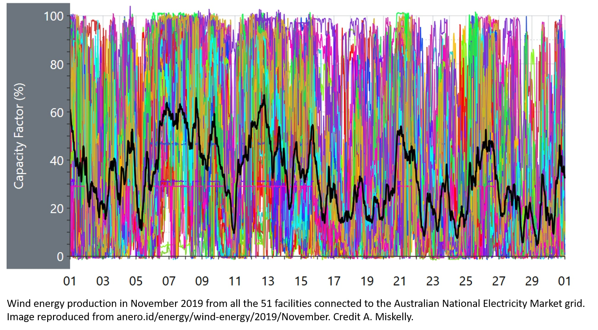
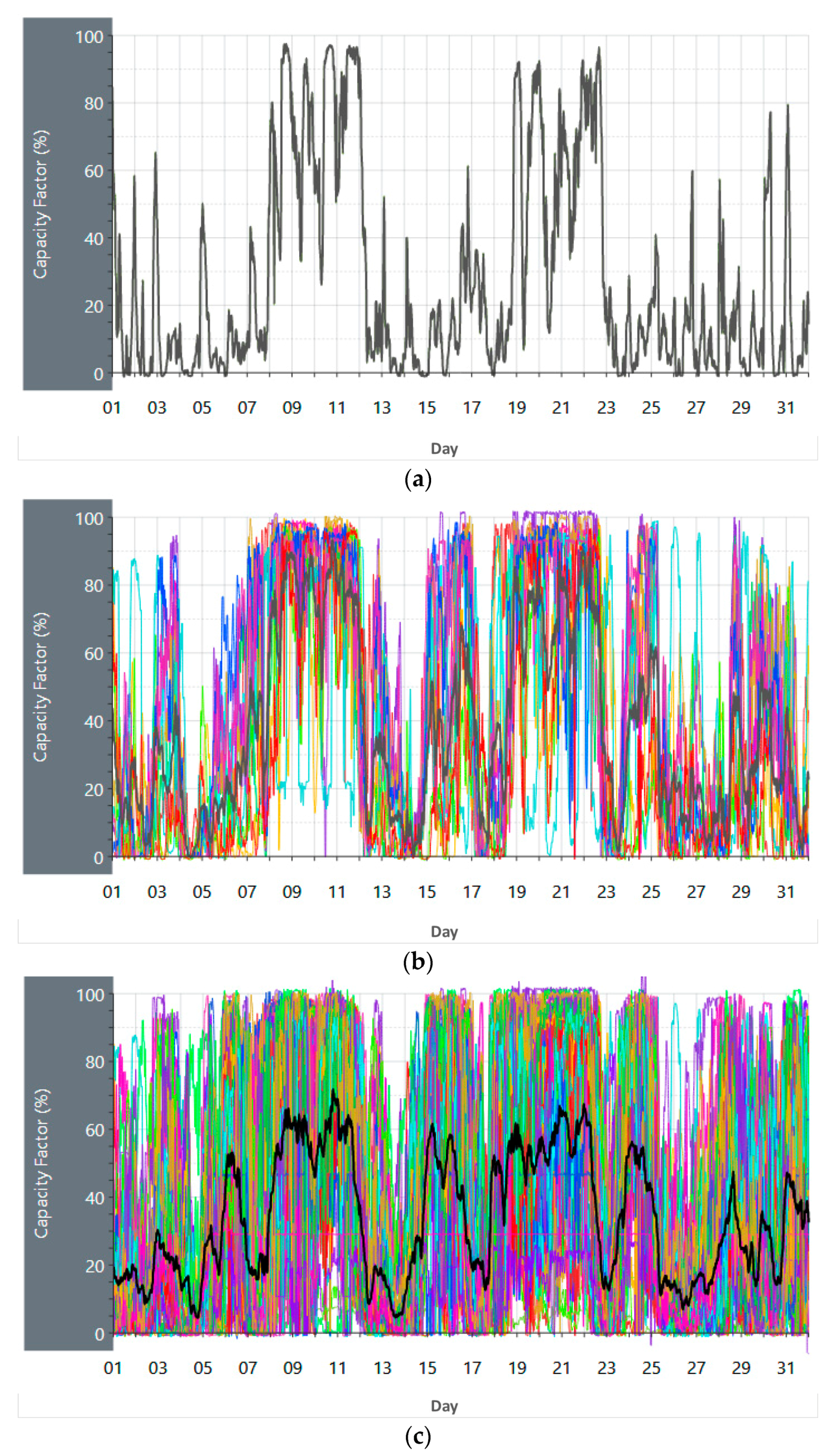
Wind energy production is characterized by significant high frequency as well as L-F variability. The H-F variability is evidenced by data collected with a frequency of 3 min or less. The L-F variability is evidenced by data collected monthly. This variability is strong for single WEF, and it remains significant for the sum of all the WEF connected to a grid, due to the strong correlation of the wind energy resource even over significant distances. If we consider for example the 40,000 km long Australian NEM grid, which is covering the populated areas of all the states and territories of Australia except Western Australia and the Northern Territory, the grid average variability of the wind energy is large, as it is shown in Figure 1 (from [48]). Figure 1a is the grid average ε for all the WEF of the NEM during August 2019. While the annual average ε is 30–35%, there are days of “highs” above 60% as well as days of “lows” below 5% ε. Figure 1b is the average ε for the WEF of one single state, in the specific case New South Wales, and Figure 1c is the ε for the largest WEF of NSW, the 270 MW Sapphire WEF. The average ε of the WEF of a single state has even higher “highs” and lower “lows”, with a situation that further deteriorates at the single facility level.

Government departments typically report of WEF proposing nominal generating power (capacity), rather than annual average actual generating power (capacity by an annual average ε). Furthermore, they do not report any parameter showing the variability. For example, Ref. [49] only reports the nominal generating power of the different WEF of Victoria. The nominal generating power of a facility is taken as the sum of the nominal power of the individual WTs. As shown by [48], the NEM WEFs work with ε, the ratio of actual to nominal power generation, over a given time window, of around 30–35% annual average. More than that, this data also shows significant variability, Figure 1, and large differences between performances of WEF, that despite having the same nominal generating power, do not work all the same. This extreme variability is the reason why electricity prices increase sharply phased with the introduction of renewable energy, as traditional combustion fuel facilities, or similar power on demand from hydro-gravity facilities, must compensate for the wind energy supply fluctuations.

Opposite to Australia, the US is covered by more widespread, but multiple, smaller grids, and there is no published H-F statistic available to understand the extent of the wind energy variability. Without the addition of massive energy storage, wind and solar photovoltaics may thus fail to produce a stable grid without combustion fuels no matter their expansion. The design of the energy storage facilities, their power, and energy requirements, may only follow a precise high and L-F statistics, to compensate fluctuations in wind energy production vs. the demand, day-by-day, month-by-month, year-by-year.

If an H-F statistic is nowhere to be found in the US, nevertheless some insight into the variability of wind energy installations in the continental, contiguous US can be found in the available monthly data by the US Energy Information Administration [50]. This variability can be investigated in time, i.e., month-by-month and year-by-year, as well as WEF-by-WEF. The aim of this paper is thus to explain the increasing discrepancy in between the growth of the installed capacity, taken the sum of the rated power of all the WTs in a facility, and the average power at which the electricity is generated in a month or a year, with ε, the ratio of actual average power by rated power, that dramatically changes from one WEF to another, by using monthly average ε. The result section will demonstrate how facilities do not work the same, for both annual averages and deviations month-by-month and year-by-year.

2. Method

Actual electricity production data in the US are available from the US Energy Information Administration (EIA) [50]. The data are available on a monthly basis since 2001, or the time of completion of the WEF, as a net generation in MWh. Annual and monthly values of ε are computed by dividing annual and monthly electricity production E by the product of the capacity P and number of hours in a year or a month n:

$${\mathsf{\epsilon }}_m=\frac{E_m}{P·n_m}$$

(2)

$${\mathsf{\epsilon }}_a=\frac{E_a}{P·n_a}$$

(3)

In these equations, E is in MWh and P in MW. The time series of the monthly capacity factors ε_m are analyzed with a simple statistic to compute the maximum, minimum, and average values over the time an energy facility has been operational. We define seasonal variability as

$${\mathsf{\delta }}_s=\frac{{\mathsf{\epsilon }}_{m,max}-{\mathsf{\epsilon }}_{m,min}}{{\mathsf{\epsilon }}_{m,ave}}$$

(4)

where ε_m,max, ε_m,min, and ε_m,ave are the maximum, minimum, and average monthly ε_m in a specific year.

We similarly define inter-annual variability as

$${\mathsf{\delta }}_i=\frac{{\mathsf{\epsilon }}_{a,max}-{\mathsf{\epsilon }}_{a,min}}{{\mathsf{\epsilon }}_{a,ave}}$$

(5)

where ε_a,max, ε_a,min, and ε_a,ave are now the maximum, minimum, and average ε_a in the time window considered. As the most part of the energy facilities considered are recent, we used 5 years of data when available, or at least 3 years of data otherwise.

While these seasonal and inter-annual variabilities are potentially useful metrics, they are far from the standard way to measure these ideas. Wind, similarly to every other climate-related parameter, is characterized by inter-annual, decadal, and multi-decadal variability (see [30,31,32]) that the limited amount of measurements collected so far mostly in recent years does not permit to determine with the due accuracy.

The effect of a variable reference wind resource can be easily modeled by using wind speed and air density data, plus the power curves of the WTs. In terms of wind speed, from latitude and longitude of every unit of a WEF complex, it is possible to download the data of reference wind speed for every month of the years of operation of the WEF unit by using, for example, the “WindSpeedData” function of Mathematica. Then, from the WT type, it is then possible to correlate the reference wind speed at the rotor axis to the power output of the WT. The wind speed then increases with height, while the density reduces. The density then follows the temperature variations across the seasons and is less affected by pressure variations. The wind speed at hub height can be extrapolated from the speed at 10 m obtained by using the “WindSpeedData” function of Mathematica by multiplying for a factor (log law). The theoretical energy production for every month is obtained by integrating in time the power computed from the given wind speed at hub height. A correction factor is also introduced to account for the monthly average temperatures at ground level that differs from the reference temperature of 293.15 K. The ground temperatures may be obtained by using the “AirTemperatureData” function of Mathematica. We take theoretical electricity production as:

$$E=\beta {\displaystyle \int }P\left(\alpha ·U\left(t\right)\right)\mathrm{dt}$$

(6)

The reference velocity U is obtained from the measurements in a nearby weather station. t is the time t. α is a correction coefficient to account for the hub height. P is a tabulated function of α·U as given in [51]. β is a correction factor for density effects. β is taken as the ratio of reference temperature for power, and the temperature from the measurements in a nearby weather station.

3. Results

The variability of wind energy production is obviously in a large part explained by the variability of the wind energy resource, as it may be inferred also when applying simple models. There are, however, other factors, namely the specific design of the facilities, that affect this variability. The aim of this paper was to show through a few cases studies the seasonal and inter-annual variability in electricity production between the largest, more recent, WEF across the US. Due to the limited number of years of data available, the inter-annual variability is computed over only 5 years of data, also accepting up to 3 years of data to increase the population. Due to the decadal and multi-decadal variability (see [30,31,32]) this short time window is not representative of any inter-annual variability, as the wind may logically oscillate with similar periodicities. Aging and maintenance of the WTs may drastically affect the production of electricity already on a decadal time scale.

To appreciate the L-F variability, we may use the data of monthly electricity production (from [50]) of WEF having about the same geographical location, and therefore falling within the same techno-resource group zone. Low frequency is therefore defined in this analysis from a month-to-month variation (seasonal variability) to a year-to-year variation (inter-annual variability). To reduce other biases, such as maintenance, only recent installations are considered. Even recently-built energy facilities have scheduled and non-schedule maintenance that contributes to downtime. Curtailment may also impact these numbers. It is finally assumed that all the electricity produced by the WEF is the electricity then delivered to the grid mentioned by [50], as it may not always be the case.

We selected the larger, more recent energy facilities, built in the US, with enough years in the EIA database to detect inter-annual variability, and electricity production figures for the different units composing the single WEF project with about the same wind energy resource. Other WEF projects with a single electricity production figure are then proposed in the following section, to further improve the reliability of the statistic of seasonal and inter-annual variability by increasing the population.

3.1. Los Vientos WEF

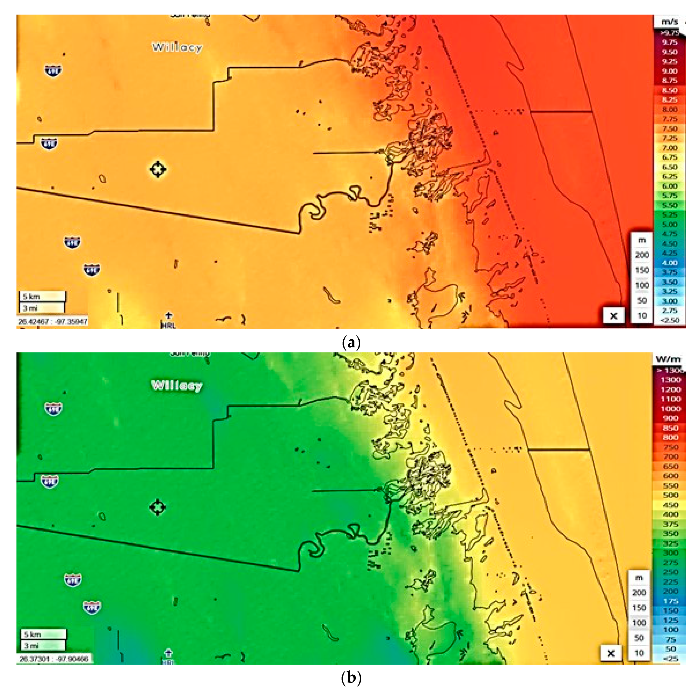
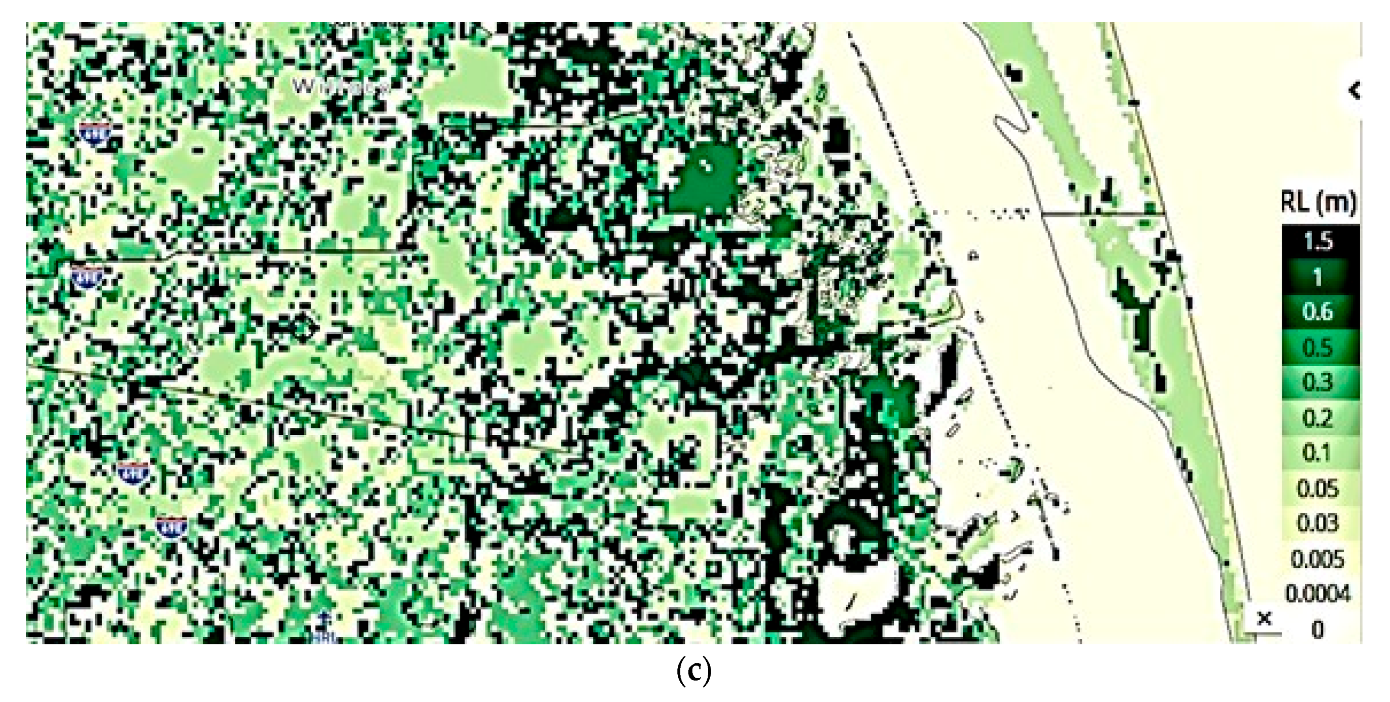
The reference power output for a given WEF unit may be estimated from the wind data for a specific location, and the power curve of the specific WT. For example, in Los Vientos (LV) 1A, the first WEF unit considered in the results section. Figure 2 presents the location and the reference wind resource at 100 m height. The roughness and ruggedness index is a measure of the steepness or roughness of the terrain. The accuracy of the wind resource reduces within complex terrains such as a mountainous area. This is not the case of LV1A.

In terms of wind speed, the location is good, but not exceptional. Then, from the WT type, in the specific case 87 Siemens SWT-2.3-101, it is then possible to correlate the reference wind speed at the rotor axis to the power output of the WT. The specific WT has rated power 2300 kW, rotor diameter 101 m and hub height 100 m [52]. This WT also has rated wind speed 12.5 m/s, cut-in wind speed 3 m/s, and cut-out wind speed 25 m/s.

As the power curve is not available for this specific WT, we might use the data of the Siemens SWT-2.3-113 [51] of the same rated power, same cut-in wind speed, same rated wind speed, and same cut-out wind speed, only differing for the rotor diameter. We assumed that the difference in rotor diameter does not change significantly the shape of the power curve. This assumption is not more questionable than neglecting the specific hub height effect when installing the WT. The same WT work differently at different hub heights.

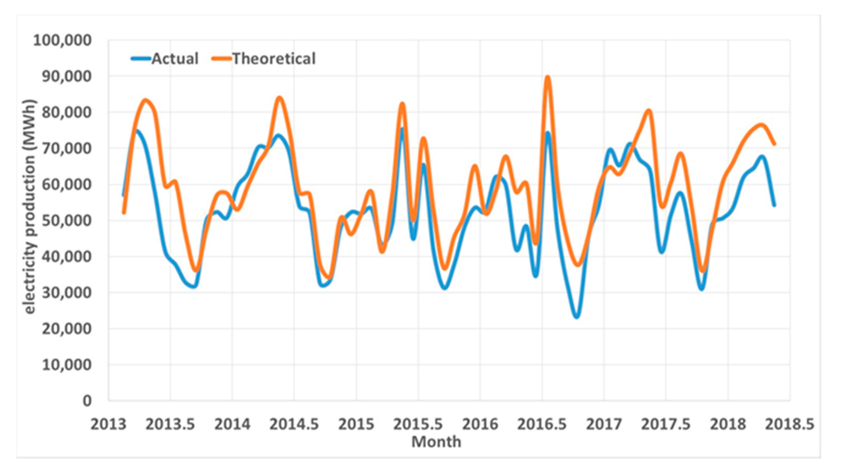
The theoretical energy production for every month is obtained by integrating in time the power computed from the given wind speed at hub height, with a correction factor to account for the monthly average temperatures at ground level. Figure 3 presents a comparison of the actual electricity production (data from [50]) and theoretical electricity production for LV1A. Despite the simplistic approach, it returns relatively close values of electricity produced, on average slightly more than the actual values.

There is a relatively good agreement between the simple evaluation of electricity production from wind speed and temperature data of a nearby weather station and the actual electricity production, with the actual electricity production that is usually 10% smaller than the theoretical value. Hence, the prevailing wind variability explains most of the irregularity in electricity production, with the specific WT power curve and hub height also contributing to the variability, with other parameters, such as orography, weather, and relative WTs’ location, affecting the detailed variation of density, velocity, and turbulence in time and in space across the rotor section of every individual WT in the WEF. As shown later, the “reference” wind variability does not explain the variability in between the performances of WEF in about the same location.

Having in mind the impact of the variability of the wind energy resource on the variability of wind energy production from a given facility, wind energy L-F variability results will then be proposed. It is expected that the wind speed and direction, and the air density may change from one WT location to the other within a WEF within short and long time-scales, producing high frequency and L-F variability. Additionally, other parameters, including the specific design of every WT, or the fluctuations of the prevailing parameters, may further contribute to high frequency and L-F variability.

The LV WEF, of the total capacity of 910 MW, is in Texas. With an output of 200 and 202 MW, the unit I (or 1A) and II (or 1B) began commercial operation in December 2012. The 200 MW unit III started operations in May 2015. The 200 MW unit IV came online in August 2016. The 110 MW unit V became operational in December 2015.

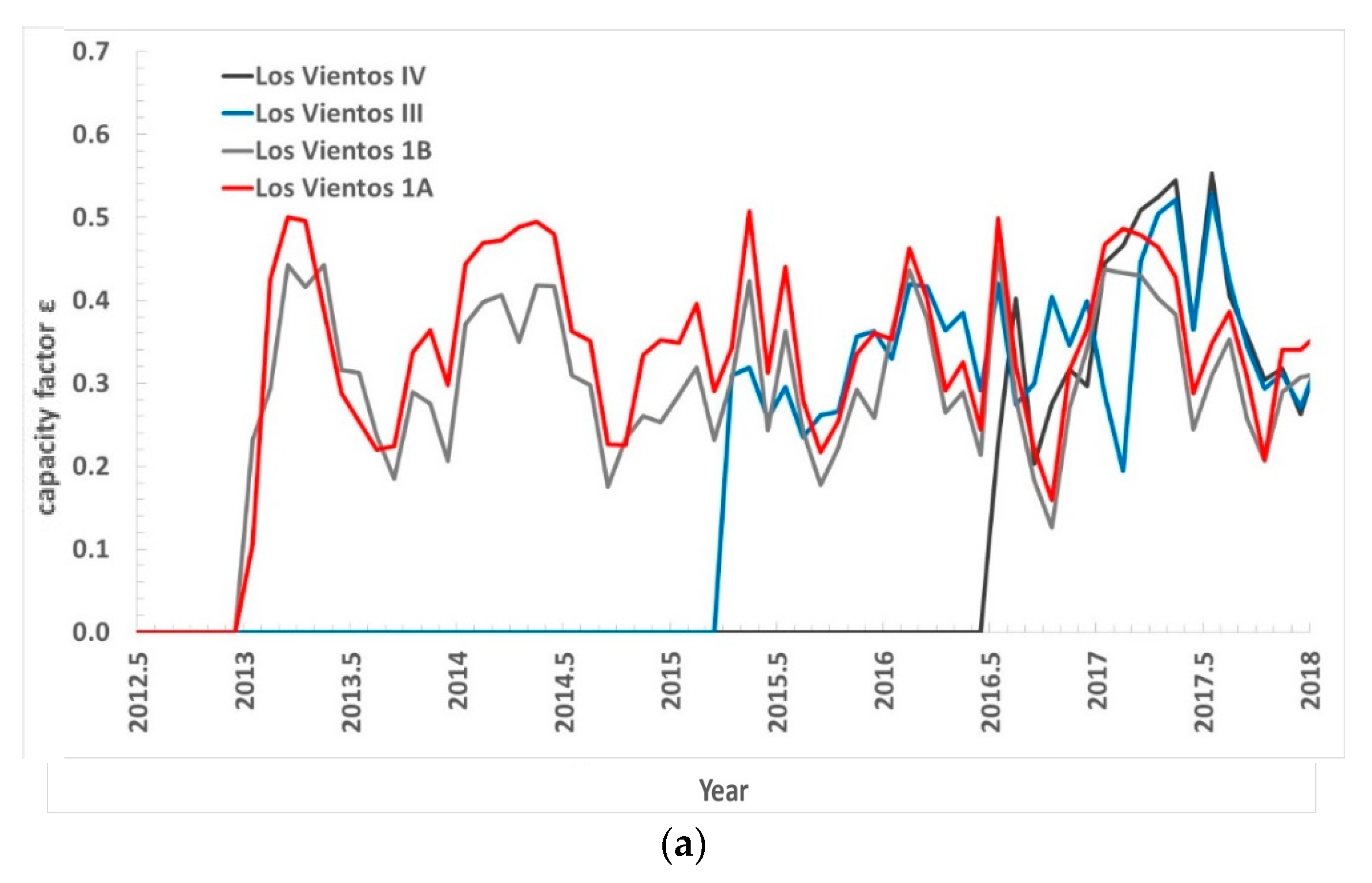
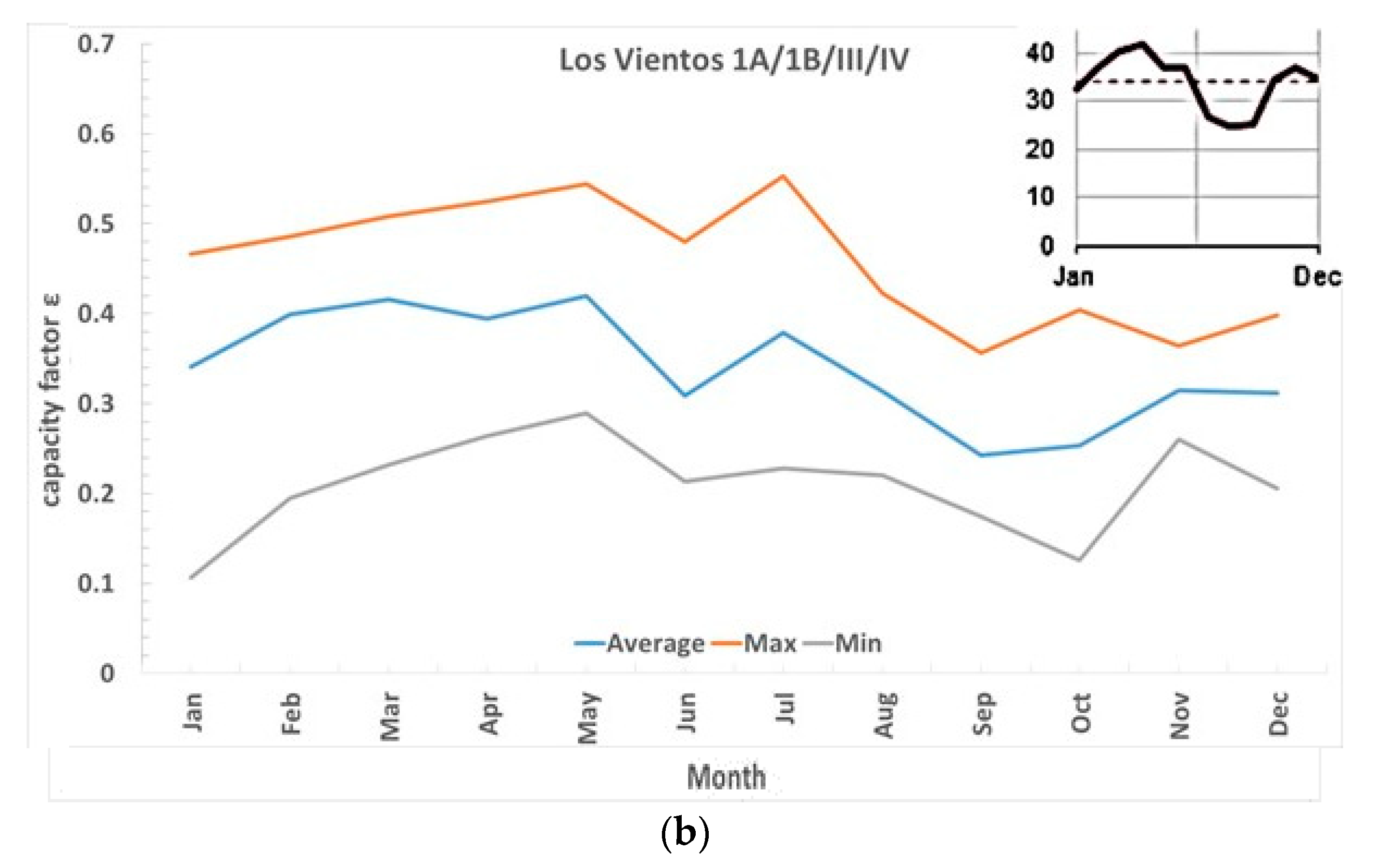
Figure 4 and

Table 2. Los Vientos (LV) wind energy complex (TX).

Energy Facility	Start of Production	P (MW)	WTs	ε 2013	ε 2014	ε 2015	ε 2016	ε 2017
LV V		110	55 Vestas V110 2 MW
LV IV	Jul. 2016	200	100 Vestas V110 2 MW					42.10%
LV III	Mar. 2015	200	100 Vestas V110 2 MW				36.23%	37.56%
LV 1B	Jan. 2013	202	84 Mitsubishi MWT 102 2.4 MW	30.40%	32.36%	28.01%	30.05%	33.72%
LV 1A	Jan. 2013	200	87 Siemens SWT 108 2.3 MW	32.39%	39.11%	34.02%	32.96%	37.79%

present ε results for the LV units 1A, 1B, III, and IV (there are no data yet for unit V). The figure also presents the reference seasonal variability for the lower plains according to [54]. The small image includes data of facilities with a net summer power >1 MW within the Lower Plains area over the period 2001–2013.

During the year 2017, maximum, minimum and average ε_m were 48.58%, 20.84%, and 37.85%, for δ_s of 73.28% in unit 1A, 43.75%, 20.63%, and 33.76%, for δ_s of 68.49%, in unit 1B, 52.81%, 19.47% and 37.42%, for δ_s of 89.09%, in unit III, and 55.32%, 26.28%, and 42.10%, for δ_s of 68.98%, in unit IV.

Over the 5 full years of data from 2013 to 2017, unit 1A had an average ε_a of 35.31%, but a maximum of 39.16% and a minimum of 32.49%. Over the same years, unit 1B had an average ε_a of 30.93%, but a maximum of 33.76% and a minimum of 28.02%. δ_i was 18.55% in unit 1B and it is 18.88% in unit 1A.

From the time series of ε_m it was evident that due to the proximity of the four energy facilities, ε_m tended to vary with a clear correlation due to the same wind resources variability, however, some energy facilities had (for example LV 1B) a systematically lower ε_m due to less optimal operation conditions of the energy facility. These effects contributed to a non-purely-statistical variability of ε_m, which may not be necessarily washed out by averaging over a larger number of sites or WEF. It is also noticed that for LV III and IV, in the last years of records, there was an improvement of ε_m compared to the start of the operation, which was due to adjustment of the operation conditions (as an example better power output control of the WTs) rather than simply better wind resources available.

The seasonal variability of LV indicates a lower energy production in September and October and a maximum production in late spring. This only partially aligned with the EIA report, where the observed ε in the year 2001–2013, for most regions of the country, were flat or increasing from January to April, then decreasing until August or September, and then increasing to the end of the year [54]. In California, however, the wind speed increased from January to June and decreased from July to December.

As shown in [5], different WTs provide a different curve for the total WT efficiency $\eta$, equation (1). The net effect is to shift up or down the curve of electricity production in Figure 3. A similar effect is produced by using a larger or a smaller hub height. By using the same reference speed of wind for all the WTs of all the WEF in LV, and the model previously described, by only changing the WT curve and the hub height, it is only possible to compute electricity production curves not intersecting each other, as it was not the case in Figure 4a. ε of LV III was sometimes above, sometimes below the values for LV I and IV. This demonstrated the limit of the proposed, classic, modeling approach.

3.2. Alta Wind Energy Center

The Alta Wind Energy Center, of 1548 MW capacity, is in California. This facility was the second largest onshore wind energy project in the world. The WTs, all from Vestas, are spread across the foothills of the Tehachapi Mountains. Units I to V were completed in April 2011. Units VI and VIII were completed in late 2011. Units VII and IX were completed in December 2012. Units X and XI were completed in 2013. Nominal capacity of the 11 units is 150, 150, 150, 102, 168, 150, 168, 150, 132, 138, and 90 MW, respectively.

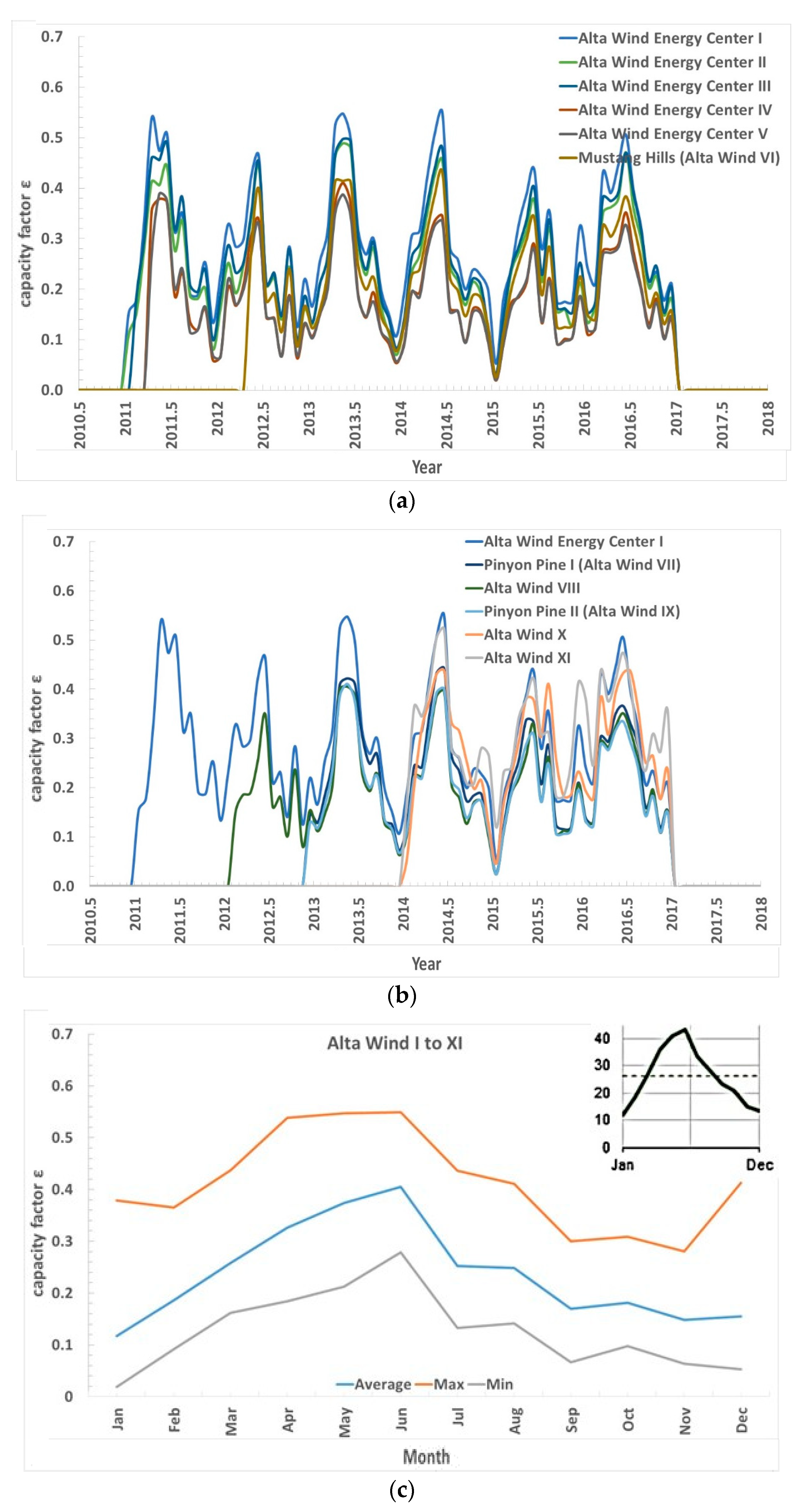
Figure 5 and

Table 3. Alta Wind Energy Center (CA).

Energy Facility	Start of Production	P (MW)	WTs	ε 2013	ε 2014	ε 2015	ε 2016
Alta Wind I	Jan. 2011	150	100 GE SLE 1.5 MW	30.36%	30.69%	25.96%	31.46%
Alta Wind II	Jan. 2011	150	50 Vestas V90 3 MW	26.55%	25.03%	21.30%	27.41%
Alta Wind III	Feb. 2011	150	50 Vestas V90 3 MW	27.48%	26.58%	22.85%	28.95%
Alta Wind IV	Apr. 2011	102	34 Vestas V90 3 MW	20.01%	18.84%	15.08%	20.52%
Alta Wind V	Apr. 2011	168	56 Vestas V90 3 MW	19.25%	18.34%	14.95%	19.93%
Mustang Hills (Alta Wind VI)	May. 2012	150	50 Vestas V90 3 MW	23.05%	23.19%	19.24%	23.94%
Pinyon Pine I (Alta Wind VII)	Dec. 2012	168	56 Vestas V90 3 MW	24.71%	24.84%	19.60%	23.56%
Alta Wind VIII	Jan. 2012	150	50 Vestas V90 3 MW	21.72%	21.52%	17.62%	22.43%
Pinyon Pine II (Alta Wind IX)	Dec. 2012	132	44 Vestas V90 3 MW	22.35%	22.10%	17.52%	21.66%
Alta Wind X	Jan. 2014	138	46 Vestas V90 3 MW		27.14%	25.59%	30.19%
Alta Wind XI	Jan. 2014	90	30 Vestas V90 3 MW		31.71%	28.18%	35.05%

present ε results for the Alta Wind Energy Center units. There was no data for the year 2017. The figure also presents the reference seasonal variability for California according to [54]. The image included data of facilities with a net summer power > 1 MW in California over the period 2001–2013.

During the year 2016, maximum, minimum, and average ε_m were 50.55%, 17.72%, and 31.38%, for δ_s of 104.62%, in unit I, 47.15%, 13.32%, and 27.35%, for δ_s of 123.69%, in unit II, 46.99%, 15.30%, and 28.88%, for δ_s of 109.73%, in unit III, 35.18%, 10.41%, and 20.47%, for δ_s of 121.01%, in unit IV, 32.72%, 10.07%, and 19.88%, for δ_s of 113.92%, in unit V, 38.36%, 13.08%, and 23.87%, for δ_s of 105.94%, in unit VI, 36.65%, 11.84%, and 23.47%, for δ_s of 105.73% in unit VII, 35.13%, 10.86%, and 22.36%, for δ_s of 108.53%, in unit VIII, 33.51%, 10.94%, and 21.58%, for δ_s of 104.58%, in unit IX, 43.62%, 17.68%, and 30.08%, for δ_s of 86.23%, in unit X, and 47.40%, 23.39%, and 34.96%, and for δ_s of 68.69%, in unit XI. Hence, δ_s of 2016 was between 68.89% and 123.69% in the different WEFs.

The annual ε_a varied between 19.93% and 35.05%. Over 6 full years of operation, the unit I maximum, minimum, and average ε_a were 31.38%, 25.92%, and 29.25% in unit I, and 27.35%, 21.25%, and 24.73% in unit II. Over 5 full years of operation, maximum, minimum, and average ε_a were 28.88%, 22.81%, and 26.02% in unit III, 20.47%, 15.05%, and 18.26% in unit IV, and 19.88%, 14.92%, and 17.81% in unit V. Over 4 full years of operation, maximum, minimum, and average ε_a were 23.87%, 19.20%, and 22.34% in unit VI, 24.87%, 19.56%, and 23.16% in unit VII, 22.36%, 17.58%, and 20.81% in unit VIII, and 22.36%, 17.49%, and 20.89% in unit IX.

Data for unit X and XI is only available for 3 full years. Unit X had a maximum, minimum, and average ε_a of 30.08%, 25.55%, and 27.59%, while unit XI was 34.96%, 28.15%, and 31.63%. δ_i was 18.68%, 24.68%, 23.32%, 29.70%, 27.83%, 20.91%, 22.96%, 22.93%, 23.34%, 16.41%, and 21.51% respectively for unit I–XI, with the largest variability 29.70% for unit IV, and the smaller variability 18.68% for unit I, and 16.41% for the more recent unit X.

At this specific location, the seasonal variability of ε_m is exceedingly high, and still quite a high variability of ε_a. The results confirm the general trend of California seasonal variability due to the climate in the region, with a maximum production towards late spring and early summer (maximum tended to be towards June, after which it fell again). In addition, larger δ_i, compared to the other cases here studied, was also observed at these sites. This might be due to other effects like the morphology of the terrain, mostly characterized by hills. The time traces of ε_m indicate a strong correlation among different energy facilities, due to the same wind resources, and even more correlation with other factors that might affect ε_m other than wind statistics. As some energy facilities consistently had lower ε_m if compared to as an example Alta Wind I and all the WTs were the same across the energy facilities, this systematic variability seemed to be associated to WT displacements/density on the land, introducing aerodynamic losses or different altitude of the WTs in the various energy facilities.

3.3. Limon Wind Energy Center

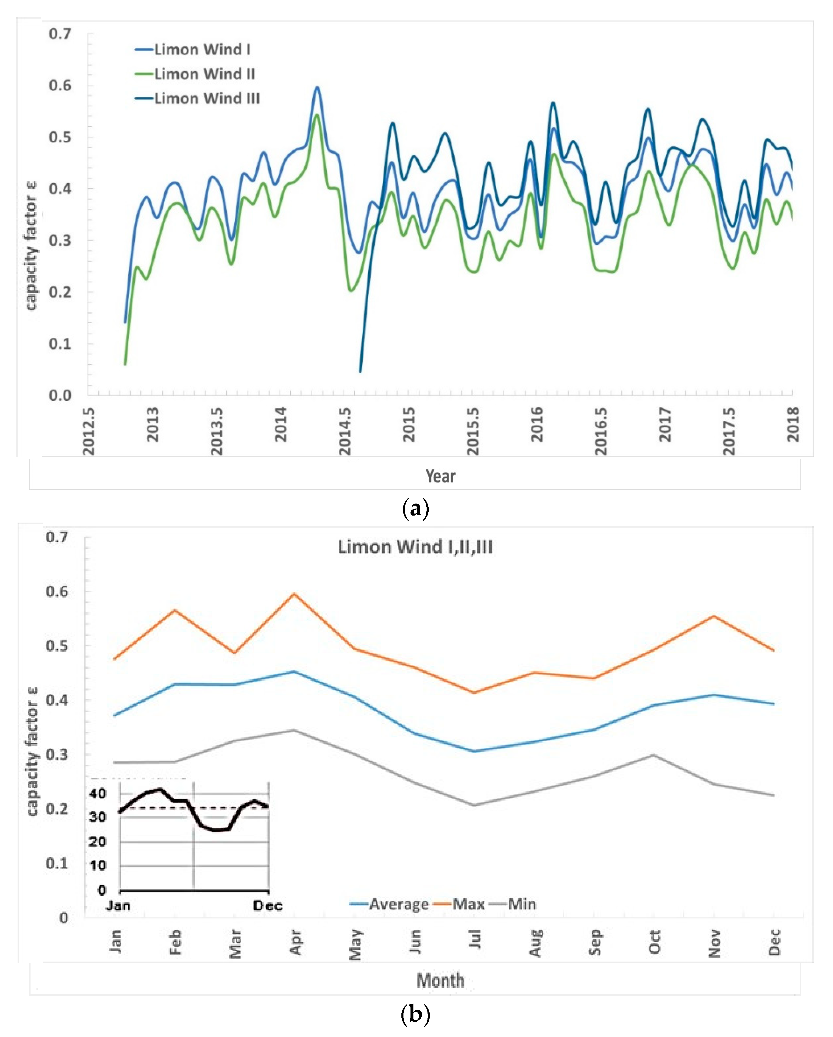
The Limon Wind Energy Center, of 605.7 MW total capacity, is in Colorado. Unit I comprises of 125 WTs GE Energy 1.6-100 of 1.6 MW of power each, for a total capacity of 200 MW. Unit II also comprises of 125 WTs GE Energy 1.6-100 of 1.6 MW of power each, for a total capacity of 200 MW. Unit III comprises of 125 WTs GE Energy 1.7-100 of 1.7 MW of power each, for a total capacity of 205.7 MW. Units 1 and 2 were completed in 2012, unit 3 in 2014. Figure 6 and

Table 4. Limon Wind Energy Center (CO).

Energy Facility	Start of Production	P (MW)	WTs	ε 2013	ε 2014	ε 2015	ε 2015	ε 2017
Limon Wind I	Oct. 2012	200	125 GE 100 1.6 MW	38.84%	42.19%	36.77%	40.02%	40.38%
Limon Wind II	Oct. 2012	200	125 GE 100 1.6 MW	34.34%	36.64%	31.22%	34.53%	35.08%
Limon Wind III	Aug. 2014	205.7	121 GE 100 1.7 MW			42.12%	43.97%	44.63%

present the electricity production and ε for the Limon Wind Energy Center units. The figure also presents the reference seasonal variability for the Lower Plains area over the period 2001–2013 [54].

During the year 2017 (the last year on record), the maximum, minimum, and average ε_m were 47.61%, 29.88%, and 40.41%, for a δ_s of 43.86%, in unit I, 44.51%, 24.62%, and 35.10%, for a δ_s of 56.64%, in unit II, and 53.45%, 32.83%, and 44.64%, for a δ_s of 46.19%, in unit III. Hence, the seasonal variability of 2017 was between 43.86% and 56.64% in the different WEF. ε_a varied between 35.10% and 44.64%.

Over the 5 full years of data from 2013 to 2017, the unit I had a maximum, minimum, and average ε_a of 42.29%, 36.71%, and 39.68%, for a δ_i of 14.05%. Over the same years, unit II had 36.73%, 31.19%, and 34.41%, for a δ_i of 16.12%. Over just 3 full years of data, 2015–2017, obviously δ_i of unit III was reduced. The maximum, minimum, and average ε_a were 44.64%, 42.10%, and 43.61%, for a δ_i of only 5.82% however it was statistically not significant. At this site, the seasonal variability tended to confirm the general trend shown in [54]. We observed similar systematic lower values of ε_m for Limon Wind I and II compared to Limon Wind III. In this case, different WTs were installed; this suggests the cause of this systematic difference, however, due to a limited number of data the statistics might not be significant.

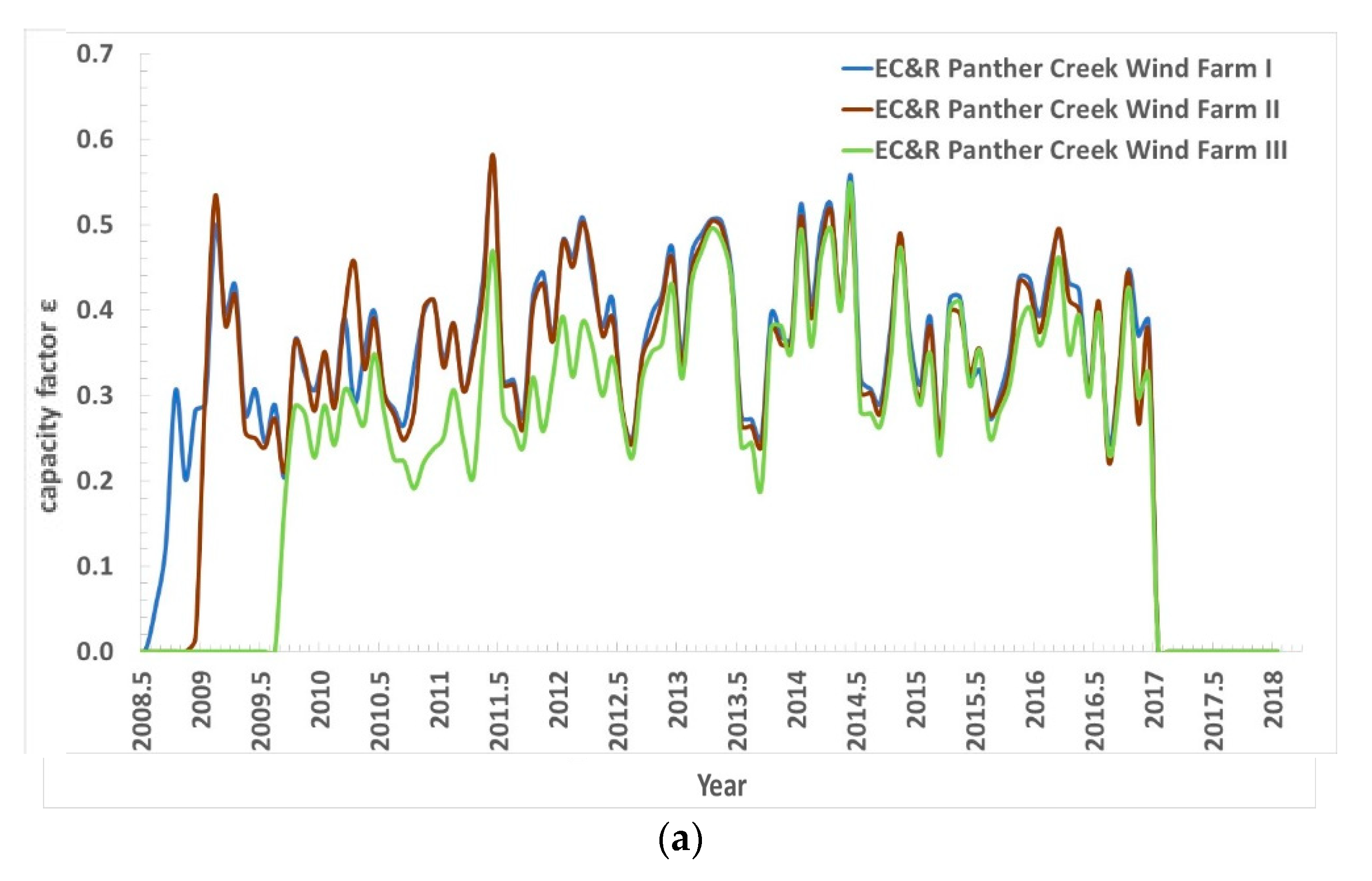
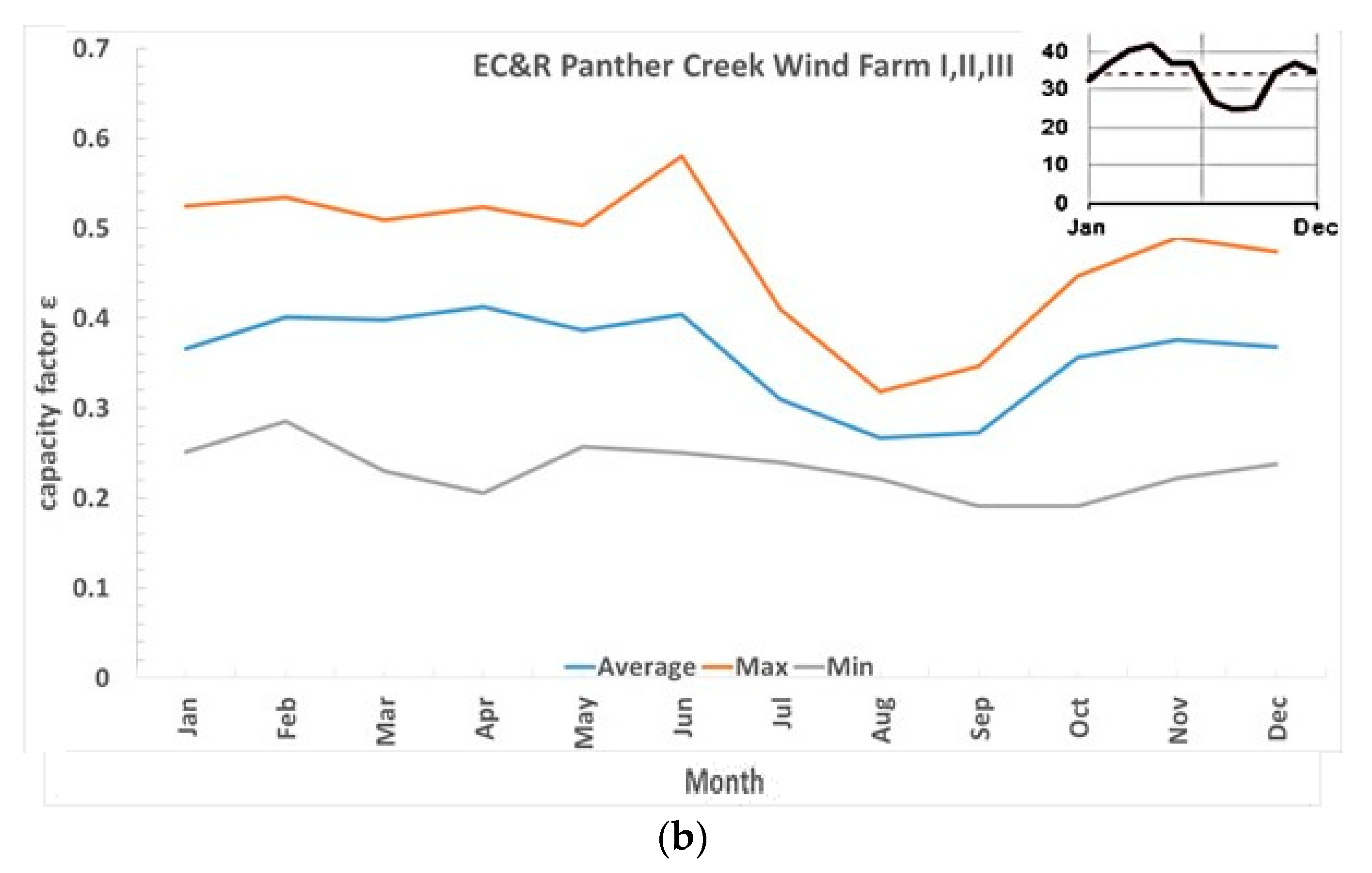
3.4. EC&R Panther Creek WEF

The EC&R Panther Creek WEF is in Texas. Unit I started production in July 2008. It has a total capacity of 142.5 MW from 95 GE 77 1.5 MW WTs. Unit II started production in December 2008. It has a total capacity of 115.5 MW from 77 GE 77 1.5 MW WTs. Unit III started production in September 2009. It has a total capacity of 199.5 MW from 133 GE 77 1.5 MW WTs. Figure 7 and

Table 5. EC&R Panther Creek Wind Energy Center (TX).

Energy Facility	Start of Production	P (MW)	WTs	ε 2013	ε 2014	ε 2015	ε 2016
EC&R Panther Creek Wind I	Jul. 2008	142.5	95 GE 77 1.5 MW	38.99%	42.07%	35.24%	38.86%
EC&R Panther Creek Wind II	Dec. 2008	115.5	77 GE 77 1.5 MW	37.98%	40.84%	34.63%	37.13%
EC&R Panther Creek Wind III	Sep. 2009	199.5	133 GE 77 1.5 MW	36.82%	39.49%	33.05%	35.30%

present ε results for the EC&R Panther Creek WEF units. The figure also presents the reference seasonal variability for the Lower Plains according to [54] including data of facilities with a net summer power >1 MW within the Lower Plains area over the period 2001–2013.

During the year 2016, the maximum, minimum, and average ε_m were 48.90%, 24.40%, and 38.88%, for a δ_s of 63.03%, in unit 1, 49.53%, 22.15%, and 37.13%, for a δ_s of 73.74%, in unit 2, and 46.15%, 23.19%, and 35.30%, for a δ_s of 65.06%, in unit 3. During the 4 years, 2013–2016, the maximum, minimum, and average ε_a were 42.07%, 35.24%, and 38.79%, for a 4-years δ_i of 17.59%, in unit 1, 40.84%, 34.63%, and 37.64%, for a 4-years δ_i of 16.51%, in unit 2, and 39.49%, 33.05%, and 36.16%, for a 4-years δ_i of 17.80%, in unit 3.

The time series of ε_m of these sites indicate much less systematic lower values of some energy facilities compared to the others. Here the WTs were all the same even if the number of WTs in the energy facility EC&R Panther Creek Wind III was much larger and the altitude effects were not to be relevant in this region.

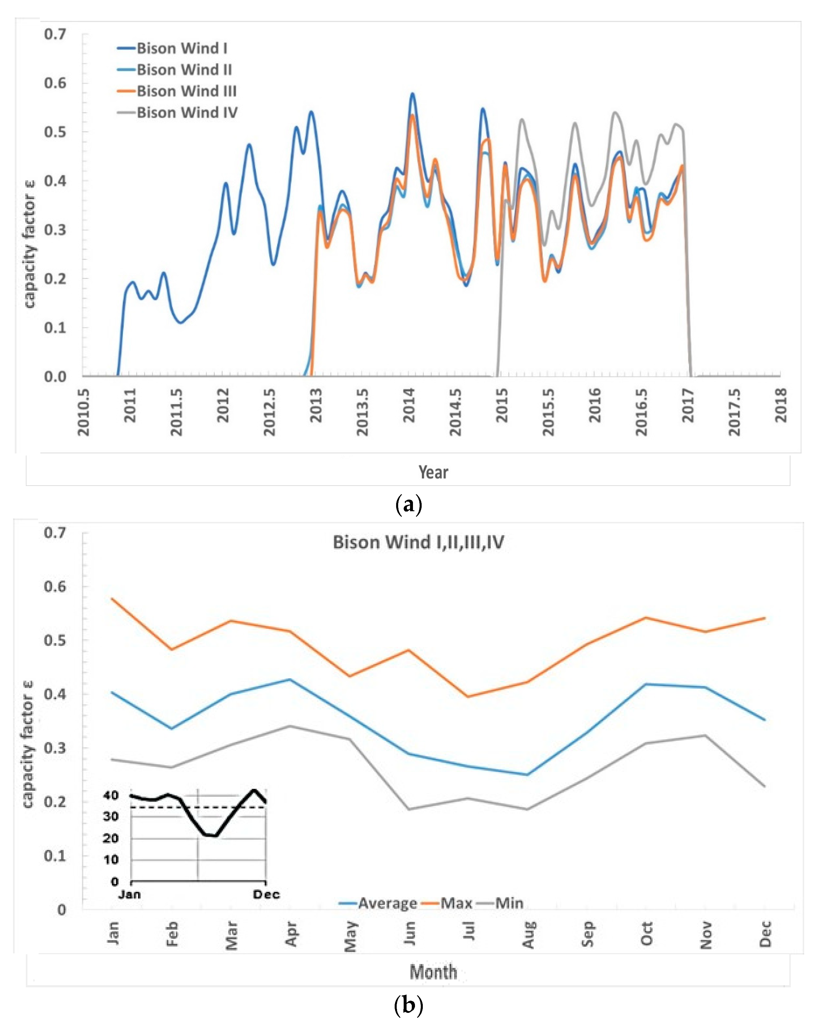
3.5. Bison Wind Energy Center

The Bison Wind Energy Center is in North Dakota. Part #1 in unit 1A was commissioned in 2010. It comprises of 16 WTs Siemens SWT-2.3-101 2.3 MW 101 m for a capacity of 36.8 MW. Part #2 also in unit 1A was also commissioned in 2010. It comprises of 17 WTs Siemens SWT-3.0-101 3 MW 101 m for a capacity of 51 MW. Part #3 in unit 1B was commissioned in 2012. It comprises of eight WTs Siemens SWT-3.0-101 3 MW 101 m for a capacity of 24 MW. Part #4 also in unit 1B was commissioned in 2011. It comprises of seven WTs Siemens SWT-3.0-101 3 MW 101 m for a capacity of 21 MW. Part #5 in unit 2 was commissioned in 2012. It comprises of 35 WTs Siemens SWT-3.0-101 3 MW 101 m for a capacity of 105 MW. Part #6 in unit 3 was commissioned in 2012. It comprises of 18 WTs Siemens SWT-3.0-101 3 MW 101 m for a capacity of 54 MW. Part #7 in unit 4 was commissioned in 2015. It comprises of 64 WTs Siemens SWT-3.2-113 3.2 MW 113 m. The total capacity is 204.8 MW. Figure 8 and

Table 6. Bison Wind Energy Center (ND).

Energy Facility	Start of Production	P (MW)	WTs	ε 2013	ε 2014	ε 2015	ε 2016
Bison Wind I	Dec. 2010	82	16 Siemens SWT-2.3-101 + 17 Siemens SWT-3.0-101	32.38%	37.57%	33.34%	37.43%
Bison Wind II	Dec. 2012	105	35 Siemens SWT-3.0-101	29.65%	35.23%	32.00%	35.75%
Bison Wind III	Jan. 2013	105	35 Siemens SWT-3.0-101	29.84%	35.52%	31.94%	35.55%
Bison Wind IV	Jan. 2015	205	64 Siemens SWT-3.2-113			39.65%	46.34%

present ε results for the Bison Wind Energy Center units. The figure also presents the reference seasonal variability for the Upper Plains according to [54]. The image includes data of facilities with a net summer power >1 MW within the Upper Plains area over the period 2001–2013.

During the year 2016, the maximum, minimum, and average ε_m were 45.76%, 29.74%, and 37.42%, for a δ_s of 42.82%, in unit 1, 44.20%, 27.91%, and 35.75%, for a δ_s of 45.57%, in unit 2, 44.55%, 28.17%, and 35.56%, for a δ_s of 46.06% in unit 3, and 53.64%, 37.39%, and 46.34%, for a δ_s of 35.07%, in unit IV

During the 4 years, 2013–2016, the maximum, minimum, and average ε_a were 37.57%, 32.38%, and 35.18%, for a 4-years δ_i of 14.73%, unit 1, 35.75%, 29.65%, and 33.16%, for a 4-years δ_i of 18.41% in unit 2, and 35.55%, 29.84%, and 33.21%, for a 4-years δ_i of 17.19%, in unit 3.

In Bison Wind, we again observed ε_m much larger for Bison Wind I and IV, compared to other sites, while the statistical variability was evident from ε_m time series varying in a similar way.

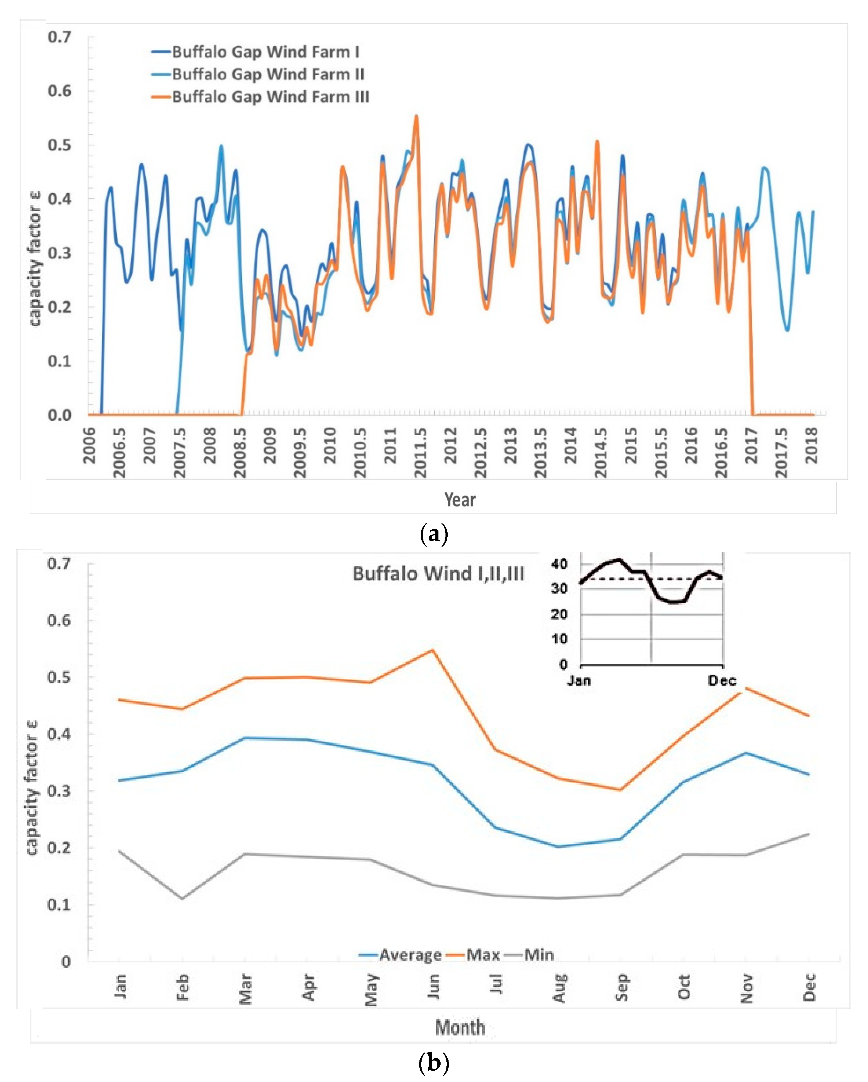
3.6. Buffalo Gap WEF

The Buffalo Gap WEF is in Texas. Commissioned in 2005, unit 1 comprises of 67 WTs Vestas V80/1800 1.8 MW 80 m. The total capacity is 120.6 MW. Unit 2 was commissioned in 2007. It comprises of 155 WTs GE 1.5 MW 77 m. The total capacity is 232.5 MW. Unit 3 finally was commissioned in 2008. It comprises of 74 WTs Siemens SWT-2.3-93 2.3 MW 93 m. The total capacity is 170.2 MW. Figure 9 and

Table 7. Buffalo Gap Wind Energy Center (TX).

Energy Facility	Start of Production	P (MW)	WTs	ε 2013	ε 2014	ε 2015	ε 2015	ε 2017
Buffalo Gap I	Apr. 2006	120.6	67 Vestas V80 1.8 MW	35.42%	36.45%	30.75%	33.08%
Buffalo Gap II	Jul. 2007	232.5	155 GE 1.5 MW	33.40%	34.63%	29.26%	33.06%	31.94%
Buffalo Gap III	Aug. 2008	170.2	74 Siemens 2.3 MW	32.85%	34.35%	28.31%	31.17%

present ε results for the Buffalo Gap WEF units. The figure also presents the reference seasonal variability for the lower plains according to [54]. The image includes data of facilities with a net summer power >1 MW within the Lower Plains area over the period 2001–2013.

During the year 2016, the maximum, minimum, and average ε_m were 44.79%, 19.83%, and 33.08%, for a δ_s of 75.47%, in unit 1, 44.25%, 20.60%, and 33.06%, for a δ_s of 71.54% in unit 2, and 42.35%, 19.53%, and 31.17%, for a δ_s of 73.21% in unit 3.

During the 4 years 2013–2016, the maximum, minimum, and average ε_a were 36.45%, 30.75%, and 33.92%, for a 4-years δ_i of 16.81%, in unit 1, 34.63%, 29.26%, and 32.59%, for a 4-years δ_i of 16.46% in unit 2, and 34.35%, 28.31%, and 31.67%, for a 4-years δ_i of 19.08% in unit 3.

3.7. Other WEF Listed as a Single Unit

Table 8. Data of other WEF of capacity >250 MW listed as a single unit.

Energy Facility	Start of Production	P (MW)	WTs	ε 2013	ε 2014	ε 2015	ε 2016	ε 2017
Biglow Canyon Wind Farm OR	Dec. 2007	450	76 Vestas v82 1.65 MW + 141 Siemens SWT 93 2.3 MW	30.21%	28.98%	26.52%	26.84%	22.70%
Rolling Hills Wind Farm IA	Jan. 2012	443.9	193 Siemens 2.3 MW	36.48%	36.08%	34.35%	34.50%	33.19%
Pioneer Prairie Wind Farm IA	Oct. 2008	300.3	182 Vestas V82 1.65 MW	36.67%	38.12%	36.70%	35.40%	36.27%
Tucannon River Wind Farm WA	Jan. 2015	266.8	116 Siemens SWT 108 2.3 MW			32.44%	37.20%
Balko Wind OK	Aug. 2015	299.7	162 GE 87 1.85 MW				42.48%	40.02%
Canadian Hills OK	Nov. 2012	298.5	62 Mitsubishi MWT 102 2.4 MW + 73 Senvion MM92 92 2.05 MW	42.09%	41.97%	35.78%	42.61%	39.91%
Grande Prairie NE	Dec. 2016	400	200 Vestas V110 2 MW					43.98%
Horse Hollow TX	Dec. 2005	736	291 GE 1.5 MW + 139 Siemens 2.3 MW	22.70%	35.81%	30.49%	33.50%	30.60%

finally presents ε results of other WEF of capacity >250 MW that are listed as a single unit. Over the 5 years 2013–2017, Biglow Canyon WEF (OR) had a maximum, minimum, and average ε_a of 30.21%, 22.70%, and 27.05%, for a δ_i of 27.76%, Rolling Hills WEF (IA) had a maximum, minimum, and average ε_a of 36.48%, 33.19%, and 34.92%, for a δ_i of 9.42%, Pioneer Prairie WEF (IA) had a maximum, minimum, and average ε_a of 38.12%, 35.40%, and 36.63%, for a δ_i of 7.43%, Canadian Hills WEF (OK) had a maximum, minimum, and average ε_a of 42.61%, 35.78%, and 40.07%, for a δ_i of 17.05%, and finally, Horse Hollow WEF (TX) had a maximum, minimum, and average ε_a of 35.81%, 22.70%, and 30.62%, for a δ_i of 42.82%.

During the year 2016, Biglow Canyon WEF had a maximum, minimum, and average ε_m of 45.61%, 9.70%, and 26.78%, for a δ_s of 134.13%; Rolling Hills WEF had a maximum, minimum, and average ε_m of 52.24%, 17.50%, and 34.62%, for a δ_s of 100.35%; Pioneer Prairie WEF had a maximum, minimum, and average ε_m of 52.45%, 15.06%, and 35.51% for a δ_s of 105.29%; Tucannon River WEF had a maximum, minimum, and average ε_m of 43.68%, 24.11%, and 37.25% for a δ_s of 52.54%; Balko Wind had a maximum, minimum, and average ε_m of 51.29%, 32.69%, and 42.51% for a δ_s of 43.76%; Canadian Hills Wind had a maximum, minimum, and average ε_m of 81.74%, 43.62%, and 63.66% for a δ_s of 59.88%; and Horse Hollow Wind Energy Center had a maximum, minimum, and average ε_m of 44.74%, 21.55%, and 33.50% for a δ_s of 69.23%. Grand Praire was not operational during all the months of 2016. In 2017, Grande Prairie had a maximum, minimum, and average ε_m of 54.56%, 28.34%, and 44.06%, for a δ_s of 59.52%. These larger WEFs show large δ_s and reduced δ_i.

Hence, within the limits of a scattered statistic from six case studies on smaller size energy facilities (from 90 to 250 MW) plus other cases of larger than 250 MW energy facilities, ε_a, as well as δ_s, and δ_i are very prominently changing across WEF of about the same location in the same techno-resource group area.

4. Discussion

A summary of seasonal and inter-annual variability of wind energy production is needed to understand the influence of the specific WEF design on these parameters. The seasonal and inter-annual variability of wind energy production is not a novelty [55]. Climatic changes are well known to produce seasonal and inter-annual variations of wind power. Temperature and pressure, and therefore density, also changes seasonally and in between one year and the other. The average, maximum, and minimum values of the monthly ε for Germany over the period 1990–2003 in [55] show an inter-annual pattern of wind power variability like the one that was shown here. The seasonal variability here shown was also close to the variability previously shown for different regions of the US [54]. The novelty of the present analysis was the pattern of variability shown across different WEF installations for about the same location, within the same techno-resource group, where the availability of wind energy is supposed to be similar. While there was a significant correlation between the different units of the same wind complex, nevertheless the annual ε might vary up to 30% between one unit and the other. δ_i changed though to a minor extent due to a time window of a few years. These inter-annual variations were also associated with energy facilities using the same WTs—as Los Vientos, Table 2 and Figure 4, or Alta Wind, Table 3 and Figure 5.

The impact of seasonal and inter-annual wind resource (and air density) variability on energy production and delivery can be reduced by agglomerating large areas where the wind patterns variability is not correlated, as this is a statistical effect. Agglomerating large area provides an apparent reduction of wind energy production variability. However, by studying WEF’s ε within similar wind resources during the years, we noticed that a contribution to this large variability could be associated with other effects than wind pattern changes.

The actual selection of WTs (variation of nominal power output and WT size), the actual arrangement of these WTs in an energy facility, their density per unit land area, and the orography of the land could be responsible for a substantial portion of changes in the annual ε as well as for changes of ε across a season and from one year to the other. This effect was not purely statistical, more systematic, thus providing a level of seasonal and inter-annual variability that could not be reduced by simply increasing the averaging areas. To reduce this further source of variability, the layout and choice of WTs should be carefully considered by optimizing the wind power output and WT selection for a given wind resource.

The actual selection of WTs and the actual arrangement of these WTs in a WEF for every specific location translated in different conditions in terms of flow parameters experienced by each WT, and the different power collected at every WT shaft. These differences might explain the changes in the annual ε, as well as the changes of ε across a season, and changes of ε from one year to the other, shown in Figure 1, Figure 2, Figure 3, Figure 4 and Figure 5.

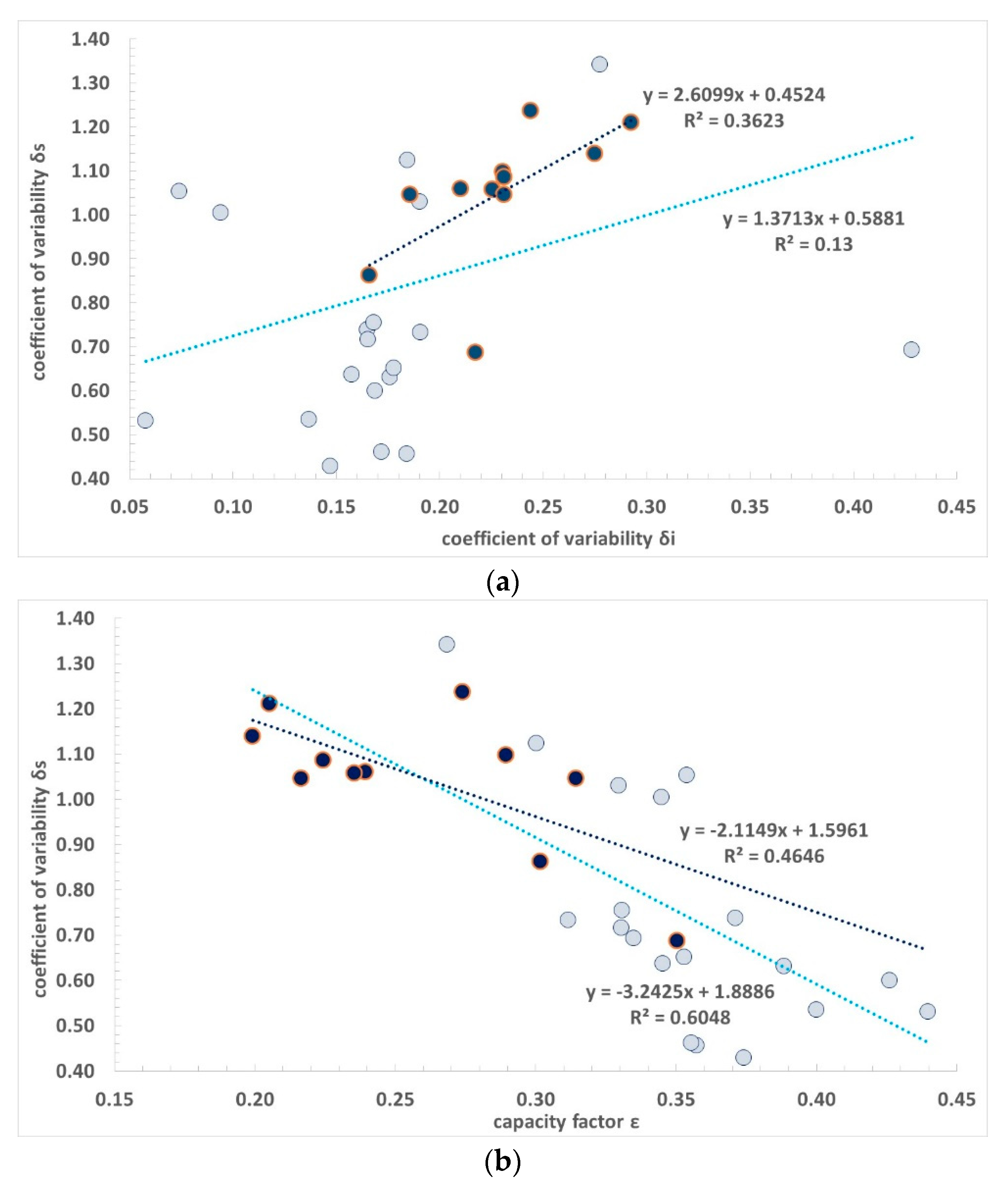
Figure 10 presents the summary results of δ_s and δ_i of the different units of WEF from Table 2, Table 3, Table 4, Table 5, Table 6 and Table 7, and of the WEF of Table 8, having a minimum of 3 years of data to compute δ_i (maximum was otherwise 5 years of data). The seasonal variability was computed for the year 2016 where most parts of the data were available, and for the year 2017 when the full year 2016 was not available. Apart from the outliers, the 3-to-5 years δ_i varied from 13% to 30%, while δ_s varied between 40% and 140%.

The 2016 δ_s correlated relatively well with the 2016 ε. R² = 0.6048. It drastically reduced as ε increased. The 5 years δ_i correlated less to the 2016 ε. R² = 0.328. It also reduced as ε increased, but less. There was some correlation also between δ_s and the 5 years δ_i, albeit with only R² = 0.13. δ_s increased if δ_i increased. The correlation between δ_s and the 5 years δ_i improved by removing four outliers to R² = 0.6409. Removal of the outliers also improved the correlation between the 5 years δ_i and the 2016 ε to R² = 0.6678, and the correlation between the 2016 δ_s and the 2016 ε to R² = 0.6639. δ_s was reducing linearly with ε, with a proportionality factor much larger than unity (values from −3.24 to −3.52). δ_i was also reducing linearly with ε, but with a proportionality factor much smaller than unity (values from −0.54 to −0.63). As the R² was very far from unity, it could be concluded that there was a limited correlation between the variability parameters and the mean value of ε.

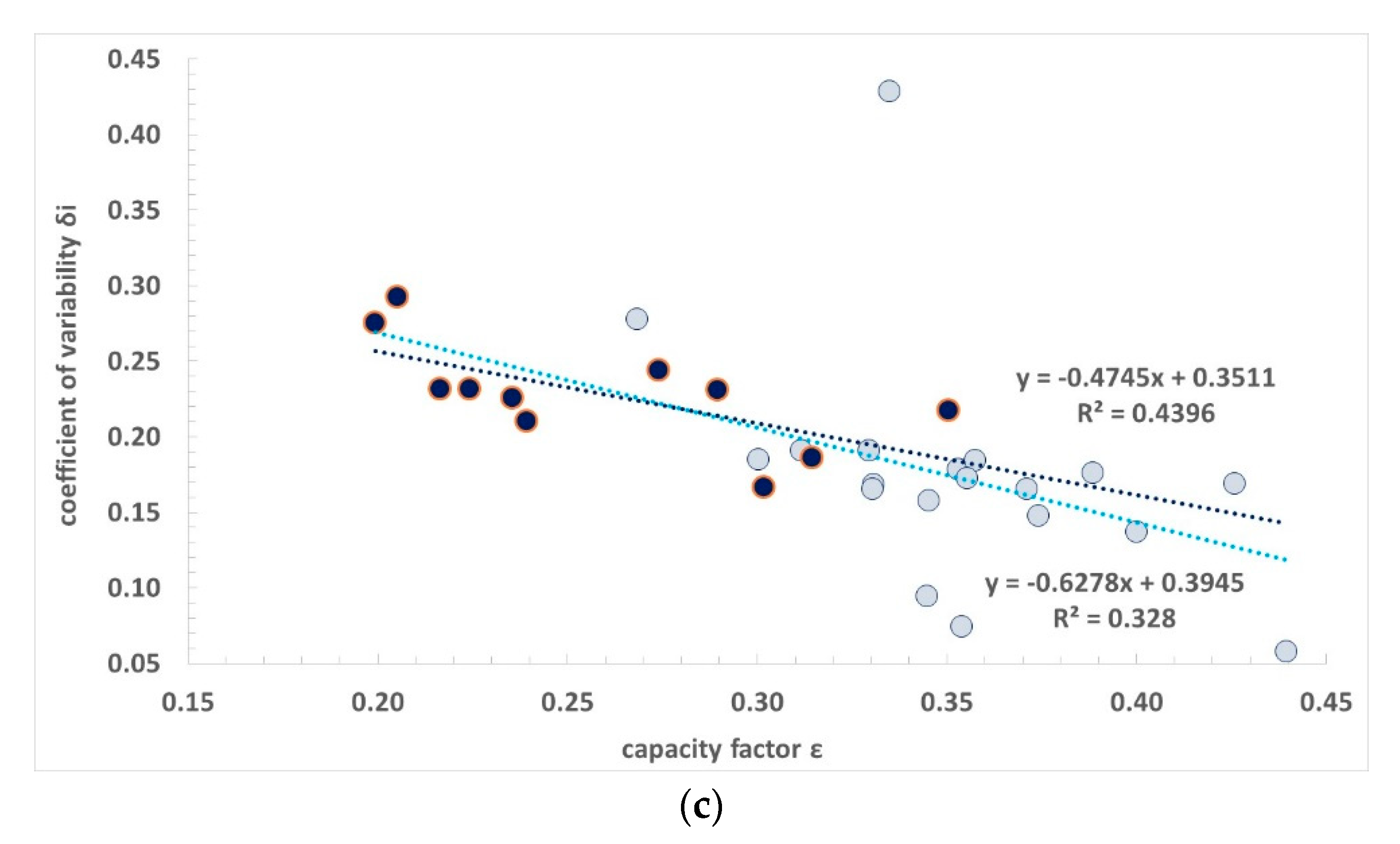
Figure 11 finally presents the summary results of δ_s and δ_i of the different units of the WEF of Table 2, Table 3, Table 4, Table 5, Table 6 and Table 7, and of the WEF of Table 8, having a minimum of 3 years of data to compute δ_i (maximum was otherwise 5 years of data), with highlighted the Alta Wind units. The 3-to-5 years δ_i varied from 13% to 30%, while δ_s varied between 65% and 125%, within nearby installations with the same WTs in all except that one unit. δ_s was reducing linearly with ε, with a proportionality factor much larger than unity. δ_i was also reducing linearly with ε, but with a proportionality factor much smaller than unity. In this case, too, the R² was very far from unity, and it could be concluded that there was a limited correlation between the variability parameter and the mean value of ε.

5. Conclusions

Wind conditions change seasonally, inter-annually, and on a decadal and multi-decadal scale. Wind energy facility performances change accordingly. However, the electricity production of a wind energy facility depends on the wind conditions experienced at any time across every rotor of every WT, and the specific harvesting (power curve) of the WTs. There is thus variability, both seasonal and inter-annual, in between wind energy facilities of different macro-regions, as well as wind energy facilities of the same micro-region, and about the same location. The extent of this variability was shown in detail in this contribution.

The variability of power generation affects the cost of electricity. It is desirable to ensure, not only, the highest possible capacity factor, a sign that the wind energy facility is producing close to the theoretical potential but also a factor that varies to a lesser extent following the inevitable oscillations of the wind energy resource. It was shown as the actual design of a wind energy facility’s impact on the annual average value of the capacity factor, as well as, to some extent, on the variability seasonally and inter-annually. A smaller mean capacity factor and a larger variability parameter both resulted in higher costs of electricity to the consumers. The tendency to reduce costs per unit installed power and the saturation of good locations for the best siting of WTs was expected to translate in reduced factors, and an increasing, rather than reducing, variability parameters of the factor. This must be compensated with improved design and adoption of extra energy storage.

In the same location, different units of the same wind energy facility complex may show different seasonal and inter-annual responses, i.e., there is a spatial variability of seasonal and inter-annual variability due to the specific wind energy facility design, as well as different annual average ε. By increasing the annual average capacity factor, the variability, both seasonal and inter-annual, somehow reduced, but with a limited correlation. Hence, there was interest to make the capacity factor as large as possible, within all the different units of the same wind complex, and to locate the wind complexes in the best locations for the wind resource, to secure larger average ε and reduced oscillations about these values.

The limited data available did not permit us to determine lower-frequency (decadal and multi-decadal) variability, but only seasonal and inter-annual variability based on a few years of data. The limited data available did not permit us to determine the more important high-frequency variability, which ultimately drives the design of the energy storage needed. More than at even lower frequencies, what is missing for the US is published data of the high-frequency variability, with sampling every minute or less, which is ultimately what is needed to understand the energy storage need of a grid.

The Levelized Cost of electricity of the wind energy must include an allowance for energy storage. A reduction in the real world Levelized cost of electricity of the wind energy may follow a better matching between WTs’ power curve and wind resource for every specific location, also addressing issues of orography, hub height, and interaction between WTs, and minimizing the transportation losses, with energy storage however necessary.

Energy storage is mandatory to benefit from wind energy (and energy of solar photovoltaics). The present performances and costs of battery storages are still inadequate, and still, in need of major improvements are the salt-water pumping hydro facilities. While upgrade of the existing hydro-gravity facilities by adding pumping is a viable short-term solution to dramatically improve energy storage capabilities, this is generally not enough to permit wind and solar grid without combustion fuels. Wind energy needs further research and development, especially in energy storage.

There is no way to fix the problem of the variability of wind energy production, as this energy production will always depend on the wind energy resource that is variable. Improvement of the design of the WTs and their optimal positioning in the given location with the better energy resources may only produce higher annual average capacity factor, and possibly somehow reduced low-frequency relative variability parameters. More than the low frequency (monthly) variability, what is relevant is the high-frequency variability, with sampling rate every minute or less. This aspect was not covered for the lack of proper data. The problem of the variability of wind (and solar photovoltaic) may only be addressed by energy storage.

Applying artificial intelligence to the wind and solar energy, as well as to energy storage, and more in general to grid demand and supplies, and pricing is becoming increasingly relevant [56,57,58], as it is, for example, the case of the many operators in the Australian National Electricity Market. Availability of resource and power generation data at the single WT level of a wind energy facility with the above-mentioned high frequency of 1 min or less, is mandatory for modelers to develop their better design of wind energy facilities and of the coupled energy storage. The way to improve the share of renewable energy in the total primary energy supply is better experimental support, better algorithms, significantly increased capacity of wind and solar, and build-up of significant energy storage, in both power and storable energy.