A Comprehensive Thermal and Structural Transient Analysis of a Boiler’s Steam Outlet Header by Means of a Dedicated Algorithm and FEM Simulation

Abstract

Increasing the share of renewables in energy markets influences the daily operation of thermal power units. High capacity power units are more frequently operated to balance power grids and, thus, steam boilers are exposed to unfavorable transient states. The aim of this work was to perform thermal and structural analyses of a boiler’s outlet steam header, with a capacity of 650∙10³ kg/h (180 kg/s) of live steam. Based on the measured steam pressure and temperatures on the outer surface of the component, transient temperature fields were determined by means of an algorithm that allows determination of transient stress distributions on the internal and external surfaces, as well as at stress concentration regions. In parallel, a finite element method simulation was performed. A comparison of the obtained results to a finite element analysis showed satisfactory agreement. The analyses showed that the start-up time could be reduced because the total stress did not exceed the allowed values during the regular start-up of the analyzed power unit. The algorithm was efficient and easy to implement in the real control systems of the power units. The numerical approach employed in the presented algorithm also allowed for determination of the time- and place-dependent heating rate value, which can be used as input data for the control system of the power unit.

1. Introduction

Fulfilling climate policy targets in the European Union has resulted in an increasing share of renewable energy in the national power systems of the member countries. The intermittent nature of renewable energy sources (RES) requires increased flexibility of power units to balance power systems and maintain the grid frequency within an acceptable range [1]. These power units usually work in off-design conditions and are started up more quickly for their design. Although this allows better integration of RES within the power grid and reduces start-up losses, which has a positive effect on overall CO₂ emissions, additional technical challenges arise for power unit operators.

Start-up procedures and quick load changes are the most unfavorable scenarios for power units in regular day-to-day use. All kinds of power units that incorporate a steam boiler or (as in the case of combined-cycle power units) steam generator, are constructed for design conditions. Therefore, in off-design conditions or during start-up sequences, the construction and pressure components work in unfavorable conditions due to the wide range of changes in operating parameters. Among these are pressure, temperature, mass flow rate of working fluid and changes in heat load absorbed by the heating surfaces in evaporators [2].

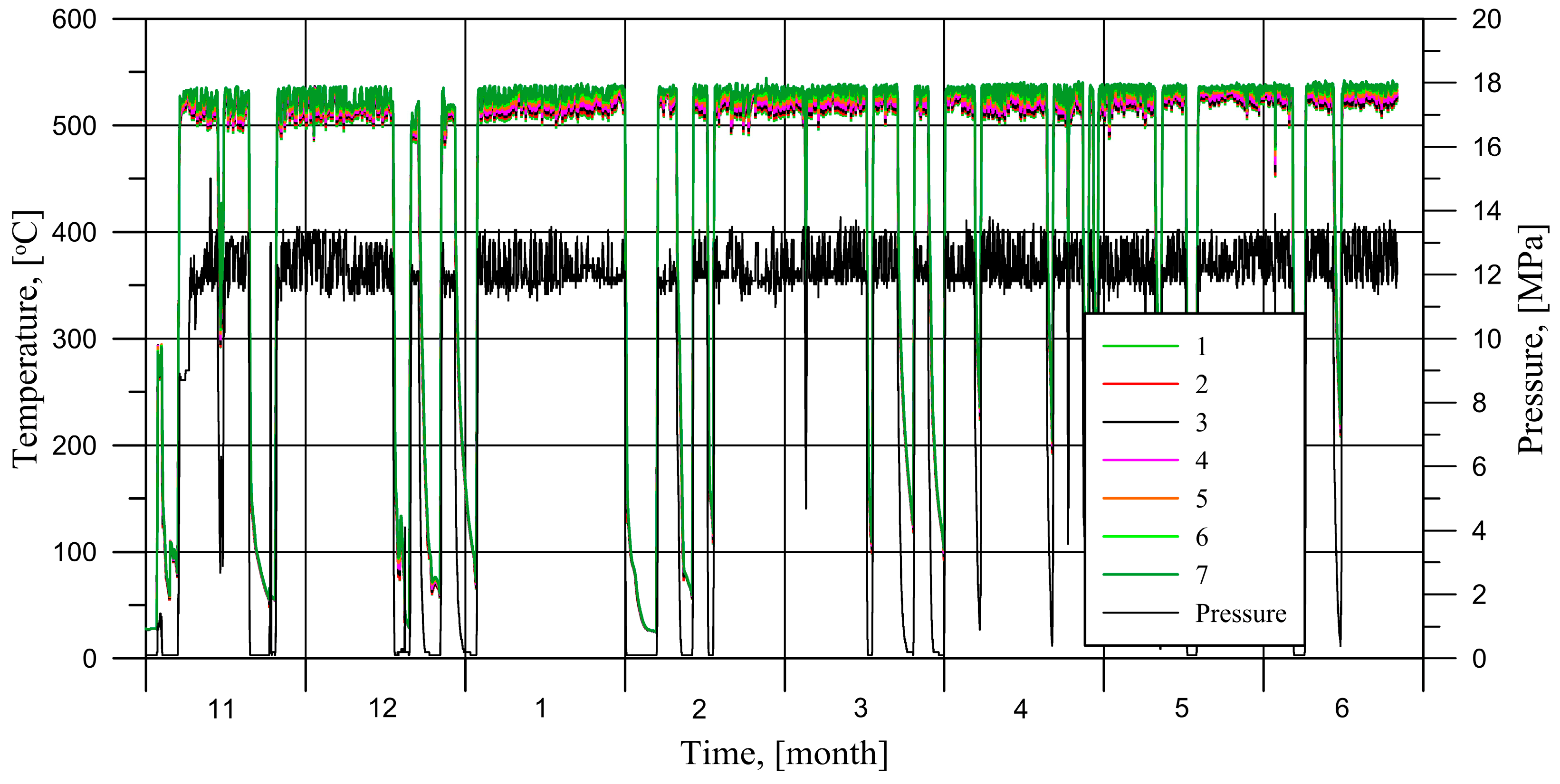
Each power unit is started up many times a year due to maintenance work and power demand fluctuations in the power grid. To illustrate this issue, Figure 1 depicts 8 months of operation of a 200 MWe power unit. The presented data consists of temperatures measured at 7 points on the outer surface of the live steam outlet header and live steam pressure. We observed that, in 8 months, this power unit was started up from an initial cold state 17 times, as well as 4 times from a warm state. One selected typical cold start-up sequence will be analyzed in this article.

The number of start-ups will increase significantly in the near future since almost all 200 MWe power units will be switched to regulation mode across Europe. For instance, as mentioned in [3], 200 MWe class units in the Polish power grid will reach as many as 200 start-up sequences yearly.

Due to the complexity of transient flows and thermal processes, the boilers’ thick-walled pressure components are subjected to considerable thermal stresses by the temperature fluctuations that occur within. Since transient thermal stresses are large enough to cause thermal fatigue and cracks, it is necessary to determine the most appropriate heating and cooling rates. Boiler manufacturers usually recommend very conservative heating rates for drums and live and reheated steam pipelines and headers. Due to the large diameters and phase change in the drums, an important parameter is the temperature difference between the top and bottom of the drum. A review of the manufacturers’ recommendations for pulverized coal-fired boilers with natural circulation is presented in

Table 1. Allowable heating rates, $v_T,$ based on manufacturers’ recommendations.

Steam Boiler’s Live Steam Capacity [103 kg/h]	Max. ∆Ttop-bottom for Boiler’s Drum [K]	Boiler Drum’s Max. Temp. Change of Steam Flow, ${\mathit{v}}_{\mathit{T}}$ [K/min]	Max. ${\mathit{v}}_{\mathit{T}}$ for Steam Pipelines [K/min]
210	60	3	4–8
230	40	1.5–2	−
380	50	1	5
650	50	1	3−5
650 (Soviet design)	40	2–4	3−6
SG & G 1	40–80	2–8	2–6

¹ Steam Boilers and Generators; recommendation of “ENERGOPOMIAR” Power Research & Testing Company.

.

The allowable heating rates, $v_T,$ are defined as a constant value for the entire start-up process or, more precisely, as a function of temperature or pressure. It should be noted that the European EN 12952-3 norm [4] is more precise and calls for higher recommended heating rates. Power unit manufacturers define allowable heating rates for thick-walled components that limit the time of start-up procedures or the value of permissible load change. Such components are called critical components and their working conditions are monitored to provide the necessary input for control systems. One such critical component is the live steam outlet header, which is a common pressure component in all kinds of steam boilers and steam generators.

Generally, control systems incorporate one or two thermocouples for monitoring the working conditions of these components. However, boiler manufacturers and power plants constantly work on adapting and exploiting power units in a wider regime of load conditions and heating and cooling rates [5]. This trend also concerns low-capacity steam boilers [6] and supercritical steam boilers [5,7]. The same approach towards the operation of power units can be observed in combined-cycle power plants. For instance, heat recovery steam generators for offshore applications have to be operated in a flexible manner in order to accommodate the variability in heat and power demands of oil and gas installations [8]. In turn, high-capacity on-shore combined cycles with heat recovery steam generators are and will be more intensively operated as load-following power units to reduce the mismatch between power supply and demand within the power grids [9]. An interesting example of a steam generator for concentrating solar power is presented in [10]. Due to the cyclic daily start-up and shut-down operation, this steam generator experiences low cycle fatigue for which it was not designed. Therefore, the authors of this paper considered this kind of fatigue and proposed a method for designing the header and heat exchanger of the steam generator by defining allowable heating rates for the evaporator.

The general need to improve power unit dynamics and flexibility brings new challenges, not just for installations, but also for control systems, which incorporate specialized algorithms for monitoring the working conditions of critical components [6,11]. These algorithms are based mainly on two thermocouples (TCs) located in the component wall [11] or on a few TCs installed on the outer insulated surfaces of critical components [6]. The latter approach is the result of general research performed in the field of power unit dynamics and on some specific power plants that implemented seven thermocouples and, consequently, upgraded control systems. Herein, it should be noted that the proposed in-house algorithm can use up to 19 thermocouples, located on one side of the cross-section of the cylindrical components.

The algorithm was validated via transient thermal analysis, in the authors’ previous works, and the method of thermal analysis was presented and discussed in [12,13]. In this article, the authors present the methodology of the structural analysis embedded in the in-house algorithm and compare the transient stress values calculated by means of the algorithm and finite element method (FEM) analysis. The transient stresses at the inner surface of the components will be analyzed, including the stress concentration region, due to the fact that the highest stresses are observed here. It should be noted that any practical implementation of such algorithms in control systems has to be proofed, and its capabilities demonstrated, in order to fulfil the industrial requirements related to accuracy and reliability. Therefore, this article demonstrates the capabilities of the in-house algorithm, which can be implemented in the control system of the power unit.

2. Steam Boiler Cold Start-up

The measured temperature and internal pressure histories that were observed during the selected cold start-up operation of the outlet header boiler will be analyzed. The OP-650 unit is a steam boiler with natural circulation, steam capacity of 650·10³ kg/h (180 kg/s), steam pressure of 13.5 MPa, and temperature of 540 °C.

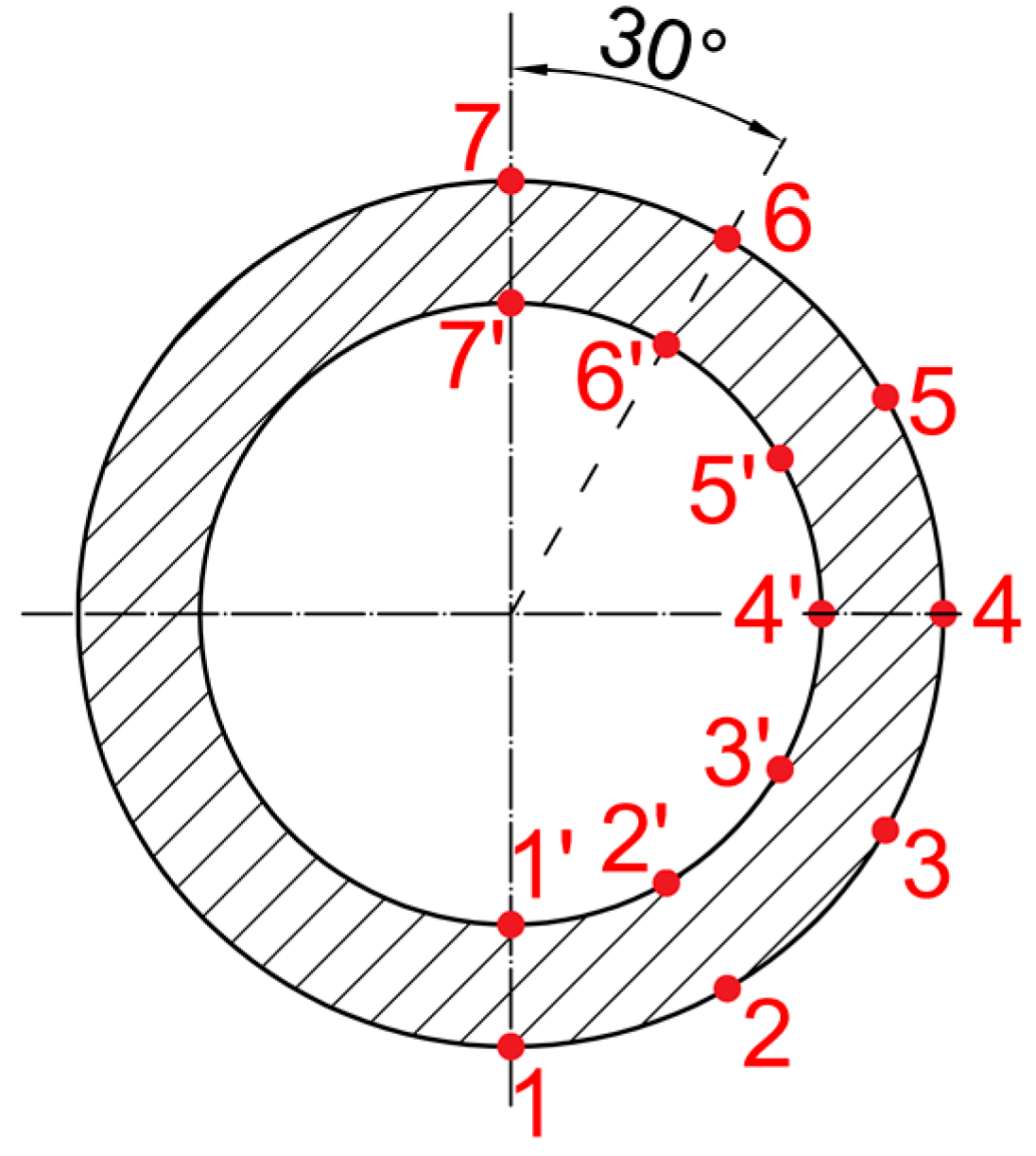
Figure 2 depicts the temperature measurement location on the outlet steam header. The outer wall surface temperatures (points 1–7) were measured using type-K thermocouples (NiCr-NiAl) with the accuracy of ±0.004·T_measured in the range 40–1000 °C. However, the specific set of TCs used in in the power plant was calibrated in order to achieve accuracy of 0.1 °C for the envisioned temperature range (in this case 0–550 °C). The pressure was measured with pressure transducers with instrumental measurement uncertainty of ±0.3% of the full scale (200 bar). Due to the symmetry of the loads, only half of the cross-section was considered. This particular set of TCs was installed to improve the accuracy and capabilities of the control system in the power plant. Normally such components are monitored with one thermocouple located on the top (point 7).

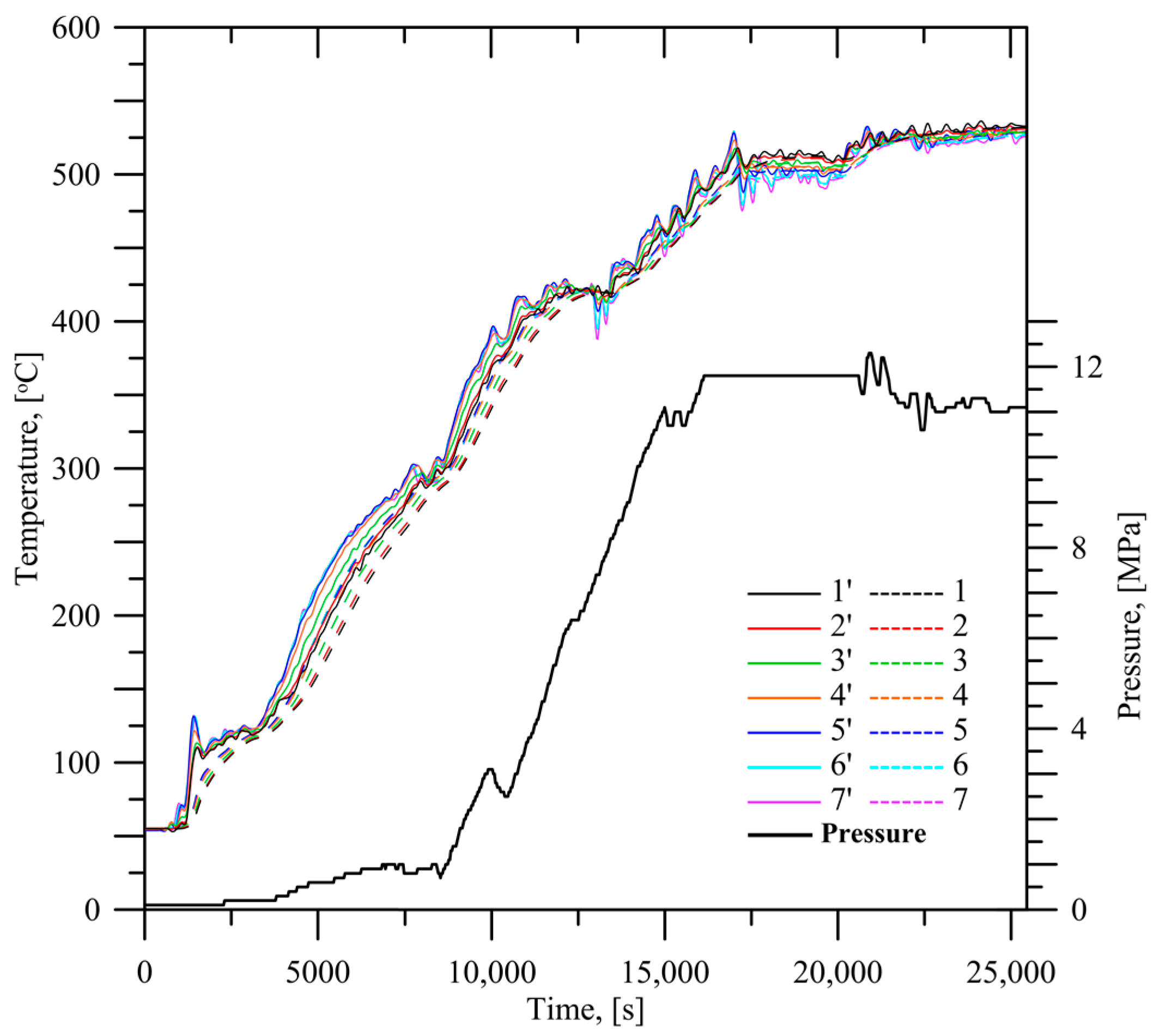
The measured temperatures at points 1–7 were taken as inputs for the algorithm. In this paper, the transient temperature and stress distributions within the outlet header were determined by means of the algorithm. The analysis considered the temperature-dependent thermal properties of steel. One of the results delivered by the algorithm was the transient temperatures at corresponding inner points 1′–7′. The algorithm was based on a solution of the inverse heat conduction problem (IHCP), solved by means of finite volume method (FVM). The minimization of measurement uncertainties on the results by means of digital filters and discretization of the half cross-section for 19 measuring points are presented in [12]. The number of input temperatures can easily be interpolated from 5, 7, 9, and 13 measuring points, up to 19. The measured input data (1–7) and the calculated temperatures (1′–7′) are depicted in Figure 3.

When analyzing the measurement data, attention should be paid to the uneven course of the temperature on the inner surface. In the initial phase of heating, the condensation of steam can be observed. After the heating process, oscillating temperature differences can be observed in steady-state operation. Such oscillations cause the thermal stresses responsible for high-cycle fatigue. Both transient and steady-state operation should be monitored by means of 7, 9 or 13 thermocouples connected with a dedicated algorithm. The maximum possible number of TCs located along the outer perimeter is 19, but for smaller diameters the distance between sensors is 1–2 cm. Therefore, the final set of sensors can be adjusted to particular cases and needs.

As mentioned previously, power unit manufacturers provide an allowable heating rate for critical pressure components. On the other hand, the EN 12952-3 standard [4] is commonly used to determine the allowable heating rates. Generally, calculations based on the EN norm are performed for the edges of the holes created by the surface of two cylinders (header–junction pipe connections), where the highest stress occurs. In this paper, the computations were performed for a junction pipe with an outer diameter of 44.5 mm and 8 mm thickness. The junction pipes are closely spaced in the element, and cracks can be observed on the edges of the holes after long-term exploitation.

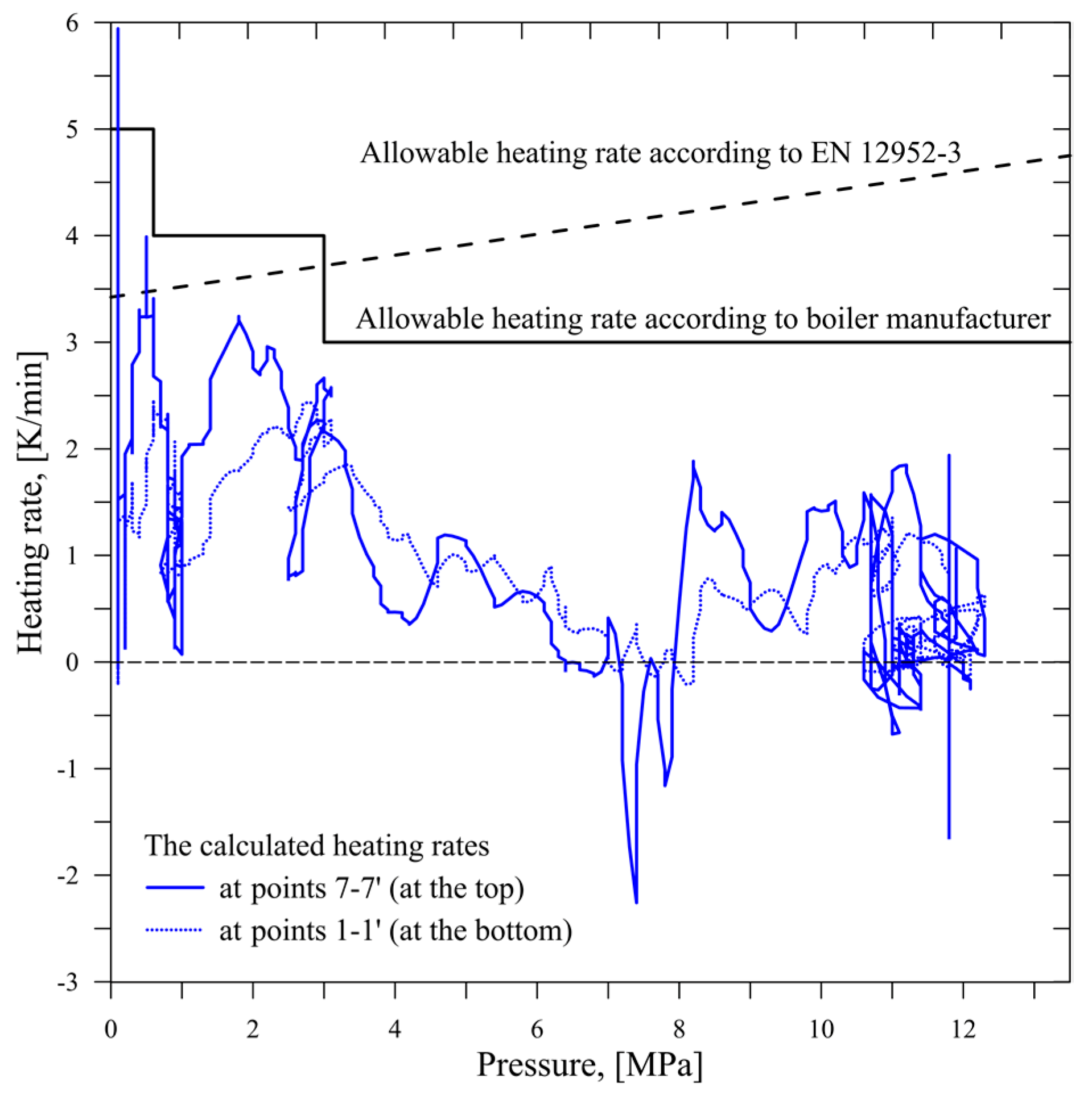
A benchmark for assessing possible improvements of boiler dynamics will be a comparison of heating rate values for the live steam outlet header. Figure 4 depicts the real values of heating rates at points 1-1′ and 7-7′, which were determined by the algorithm based on the measured data. The real heating rates are compared to those delivered by the manufacturer and calculated based on the EN norm. More information regarding EN norm calculations can be found in [4] and [14].

The calculated temperature transients were obtained from Equation (3) according to the data shown in Figure 3. When analyzing the data shown in Figure 4, it can be stated that the real header heating rate values show significant irregularity and stay within the allowable scope according to the EN standard and the manufacturer’s recommendations. Only at the beginning of a start-up operation, when the gauge pressure barely exceeds 0 MPa, were the allowable heating rates exceeded. This was slight, short-lived, and caused by the steam condensation process. However, from the point of view of the stresses within the outlet header, the start-up procedure can be shortened. To provide a better overview, such analysis should be performed for all critical components of the boiler in order to comprehensively assess the possibilities of reducing start-up times.

3. Thermal and Structural Analysis of The Boiler’s Steam Header

The thermal and structural analysis was performed using Ansys software [15]. The analysis results were compared with the results delivered by the algorithm. The input data used in the analysis were adopted from Figure 3. The outlet steam header was made of low alloy steel of 10CrMo910 grade. The outer diameter, wall thickness, and the discrete model length were 508 mm, 100 mm, and 920 mm, respectively. The discrete model included all the connection pipes welded to the steam header. The temperature-dependent thermal properties of the low alloy steel were taken into account during the analysis.

3.1. FEM Analysis of the Header

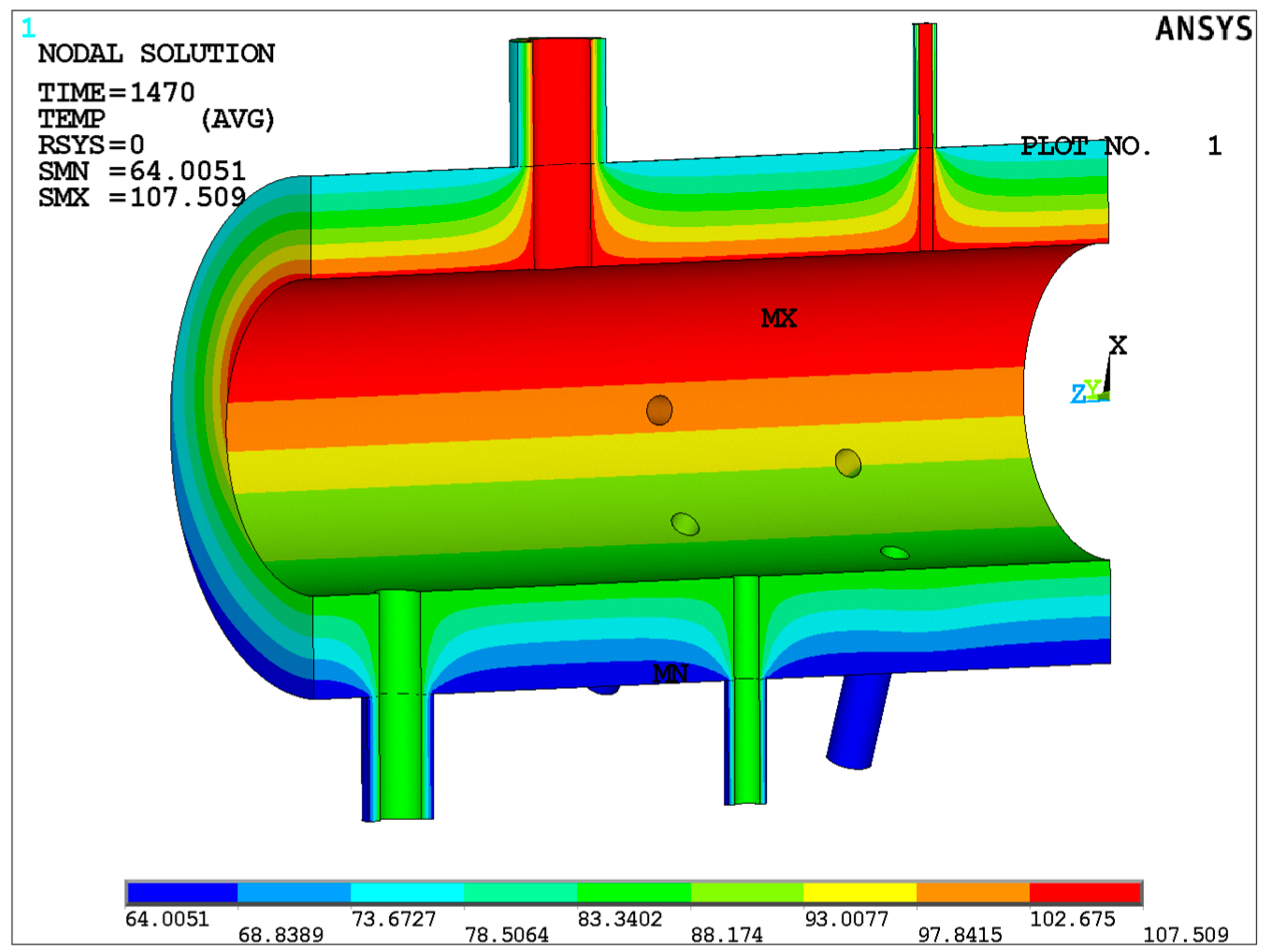
The FEM analysis was performed using Ansys Mechanical ADPL v. 19.0. The mesh grid of the discrete model consisted of 138,354 finite elements, which made it possible to satisfy a grid independence study. Based on the temperature values from Figure 3, the temperature distribution within the entire steam header wall was determined. Figure 5 depicts the temperature field within the pressure component for the time τ = 1470 s. The highest thermal stresses were observed for this time step.

The temperature distributions determined from FEM analysis allowed the structural analysis to be performed. The obtained temperature fields were considered as thermal loads in the structural analysis for each time step. Steam pressure was applied as the boundary condition at the inner wall surface. The equivalent pressures on cross-sections of the header and junction pipes were also applied.

3.2. In-House Algorithm

The algorithm allowed the transients of axial, hoop, total stresses at the inner and outer surface, and the edges of the holes to be determined (created by the header and junction pipes). The algorithm combined equations for thermal stresses derived via an assumption of quasi-state heating and correlations for stress concentration factors defined in [4]. Stress concentration factors α_m and α_t allowed for the determination of mechanical and thermal stresses at the aforementioned edges. To provide an accurate and reliable calculation of stresses and heating rates, the algorithm incorporated transient temperature differences calculated on the basis of the solution of the inverse heat conduction problem. This meant that the current heating rate was calculated based on the temperature difference $\Delta T_{o-i}$ (Equation (3)). The basic equations related to the inner surface are presented below to provide better insight into the applied approach.

Assuming that the thermal load of the element was axisymmetric, and that the ends of the tubular element could move in an axial direction, the axial and circumferential stresses on the inner surface were expressed by the following Equation (1) [16].

$${\sigma }_{th,1i}= {\sigma }_{th,2i}=\frac{E\alpha }{1-\nu }\Delta T_i$$

(1)

The following formula gives the temperature difference $\Delta T_i$:

$$\Delta T_i=v_T\frac{s^2}{a}{\varphi }_i$$

(2)

where $v_T$ is the heating rate calculated from Equation (3), and ${\varphi }_i$ is the shape coefficients determined for the inner surface, given by Equation (4) [16]:

$$v_T=\frac{2a\Delta T_{o-i}}{0.5\left(r_o^2-r_i^2\right)-r_o^{2}ln\left(\frac{r_o}{r_i}\right)}$$

(3)

$${\varphi }_i=\frac{1}{8}\frac{\left(u^2-1\right)\left(3u^2-1\right)-4u^{4}ln\left(u\right)}{\left(u^2-1\right){\left(u-1\right)}^2}$$

(4)

For the given temperature difference across the tube wall, $\Delta T_{o-i}$, the thermal stresses can be determined from Equations (1)–(4). The inner surface circumferential stresses, ${\sigma }_{mech,1i}$, induced by pressure inside the thick-walled axisymmetric cylindrical component were determined using the the Lamé formula.

Using the superposition principle, the thermal stress produced by the temperature gradient across the wall thickness could be added to the mechanical stress derived from the pressure, according to Equation (5) [17].

$${\sigma }_{total,i}={\sigma }_{mech,1i}+{\sigma }_{th,1i}$$

(5)

The stress concentration factor, which describes the change of thermal stresses, is given by Equation (6) [4].

$${\alpha }_{th}=\sqrt{{\left[2-\frac{h+2700}{h+1700}z+\frac{h}{h+1700}\left(e^{-7z}-1\right)\right]}^2+0.81z^2}$$

(6)

where z is the average diameter of the junction pipe to the average diameter of the outlet header ratio. According to the norm [4], the heat transfer coefficient h was taken depending on the water phase in the pressure component: h = 1000 W/(m²·K) for steam and h = 3000 W/(m²·K) for water.

The thermal stresses occurring at the hole’s edge may be calculated using Equation (7).

$${\sigma }_{th,e}= {\alpha }_{th}\frac{E\alpha }{1-\nu }\Delta T_i$$

(7)

$${\sigma }_{total,e}={\sigma }_{th,e}+{\alpha }_{mech}{\sigma }_{mech,1i}$$

(8)

Total mechanical and thermal stresses at the hole’s edge may be determined using Equation (8).

4. Results and Discussion

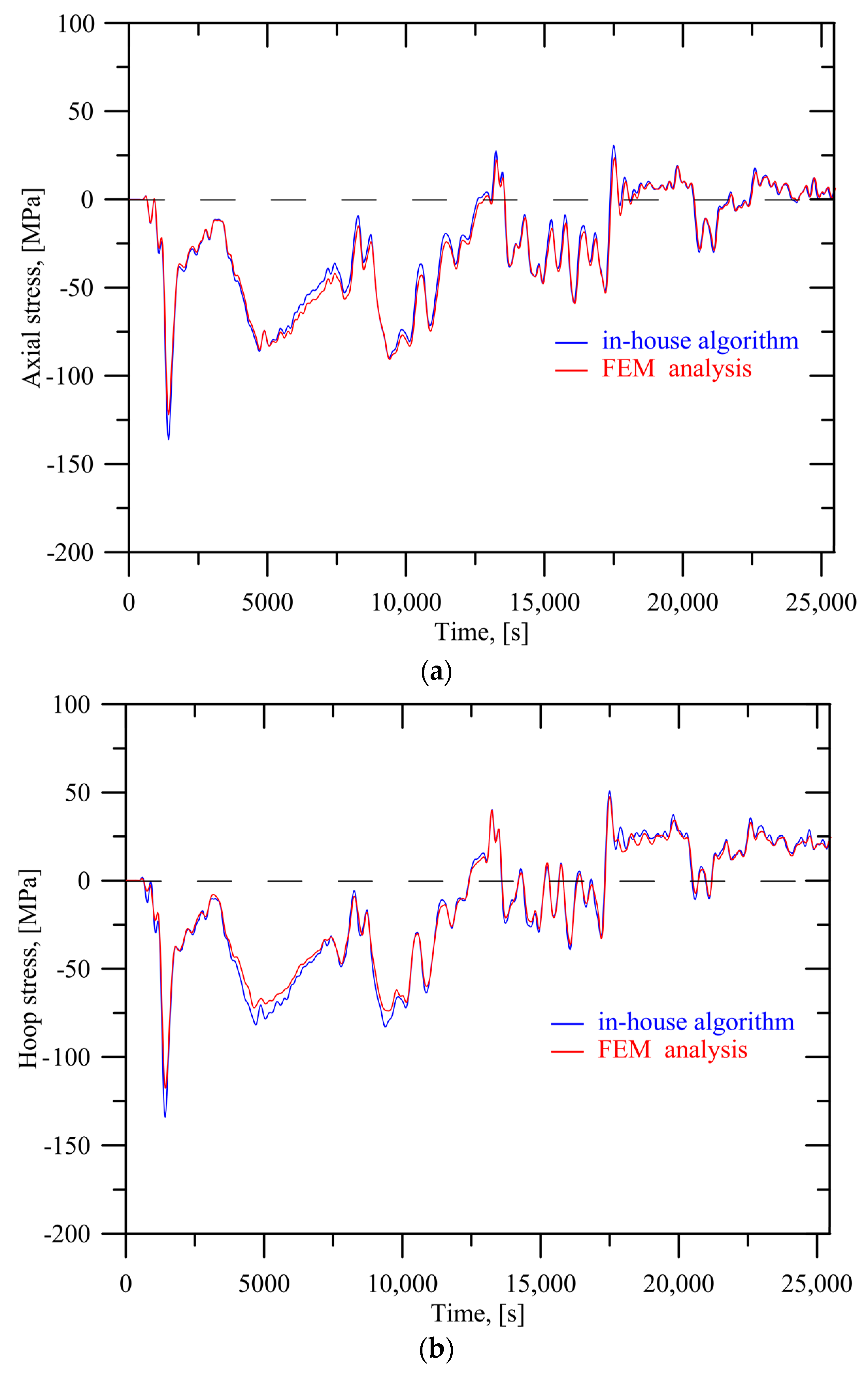
The results of the algorithm-based analysis were compared with the FEM analysis. Figure 6a,b shows the values of the axial and circumferential stresses on the inner surface (point 7′) of the steam header during a cold start-up.

Very good agreement between the presented methods was found. The highest stress value was −135 MPa; thus, the pressure component operated in an elastic strain region.

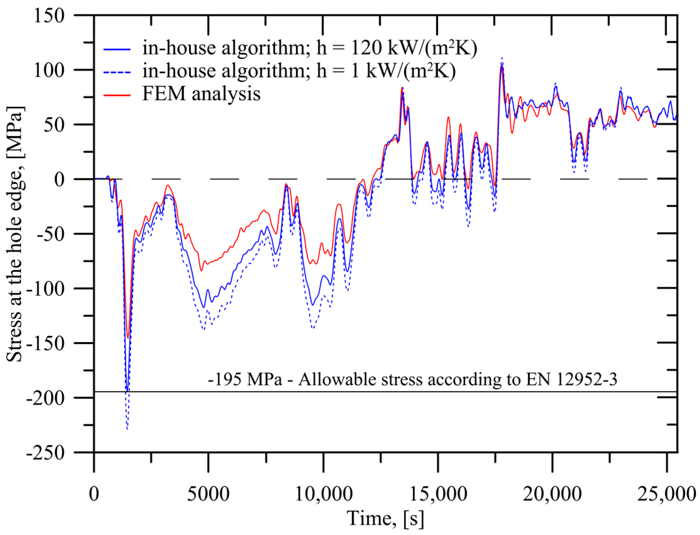
The results for both the algorithm-based and the FEM methods for the edge of the junction pipe are shown in Figure 7.

Since the highest stresses occur in the stress concentration regions, the EN 12952-3 standard allows determination of the permissible stress value for this region during start-up, which was −195 MPa for the analyzed case. Moreover, the stresses were calculated using algorithm and FEM-based analysis. The thermal FEM analysis considered the temperature distributions determined by means of the in-house algorithm. Thus, the thermal analysis did not require knowledge of the values of parameters such as heat flux or heat transfer coefficient, which are difficult to measure in practice in such components. The mechanical FEM analysis was then performed considering necessary boundary conditions and the internal pressure variation. Figure 7 shows the stress courses for the two selected values of heat transfer coefficient h employed in the in-house algorithm. According to the EN 12952-3 norm, the heat transfer coefficient h was assumed to be constant at the inner wall circumference during the entire start-up operation. For h = 1000 W/(m²·K), the agreement between the methods was not satisfactory. The differences in the predicted values were as much as 85 MPa, which was the result of the simplified assumptions adopted from the EN norm. According to the assumption delivered by the norm, the value of h = 1000 W/(m²·K) should be reconsidered. In the initial start-up phase, the water vapor condensed on the inner surface of the header. Therefore, the heat transfer coefficient may exhibit a significant increase, reaching 120,000 W/(m²·K) in extreme cases during nucleate condensation of steam [18]. Calculations that assume a higher h value provide significantly better compatibility with the results of the FEM simulations. However, the heat transfer coefficient varies across a wide range of values and is not constant during transient states. The simplification to two constant values of h adapted by the EN norm shows that the h parameter is basically an artificial parameter that can tune the outputs rather than present a heat transfer coefficient itself. This is especially true when the lower values of h = 1000 or 3000 W/(m²·K) from the EN norm, overestimate the stress values determined on the basis of the transient temperature difference $\Delta T_{o-i}$. In pressure components such as steam outlet headers, flowing steam has high temperature and pressure. In addition, steam flows out of different sections of the steam superheater (via junction pipes). Therefore, it is hard to recognize one uniform steam flow; this results in significant practical difficulties when attempting to determine the heat transfer coefficient at the inner surface of the outlet header.

The advantage of the presented approach was the use of the temperature values measured on the easily accessible outer surface of the component and the calculation of transient temperature and stress distribution within the component. Although the algorithm is for solid hollow cylinders, the performed analysis showed that the stress values at the edge of the hole were reasonable during transient states but higher than those obtained from FEM analysis. It should be noted that the degree of agreement between detailed FEM analysis and the algorithm’s results were fully satisfactory in normal operation of the power unit (nearly steady-state conditions). The algorithm was fast and efficient owing to the fact that computational effort for a regular PC (4 cores, 16 GB RAM) is about 3 s per 1 h of measured real data. In comparison, thermal and structural FEM analysis takes about 1–1.5 h and requires substantial disc space (in this case, the size of the analysis of each 5000 s of the measured data took around 70–90 GB of disc space).

5. Conclusions

This paper presents the thermal and structural analysis of an OP-650 boiler’s steam outlet header. The analysis was based on data acquired during the boiler’s start-up from a cold state. Circumferential and axial stresses on the inner surface of the pressure component were determined by means of an in-house algorithm and FEM simulation. Based on the performed work, the following conclusions can be stated:

• The presented approach combining the algorithm and FEM analysis is an effective method for acquiring detailed assessment of the working conditions and total stress values within critical components of power units.
• On the basis of the real values measured during a typical start-up operation of a power unit, we were able to ascertain whether or not acceptable stresses were exceeded. This allowed for assessment of existing margins to improve the flexibility and start-up times of power units.
• The algorithm calculated transient characteristic temperature differences within the analyzed component and, thus, allows for quick and efficient calculation of transient thermal and total stresses.
• Stress concentration factor α_t allows for determination of thermal stresses in stress concentration regions, but the results were overestimated during transient states. However, for lower heating rate values of |$v_T$| ≤ 1.5 K/min, the algorithm provides fully satisfactory convergence with the FEM-based analysis. For higher heating rate values we recommend an adaptation of α_t based on FEM-based analysis.
• Thanks to the quick and efficient thermal and structural computations, which were based on up to 19 temperature measuring points located on the outer surface of the monitored component, the presented algorithm can be integrated with the control systems of power units.