Optimal Management of Combined-Cycle Gas Units with Gas Storage under Uncertainty


Abstract
:1. Introduction
2. Model Description
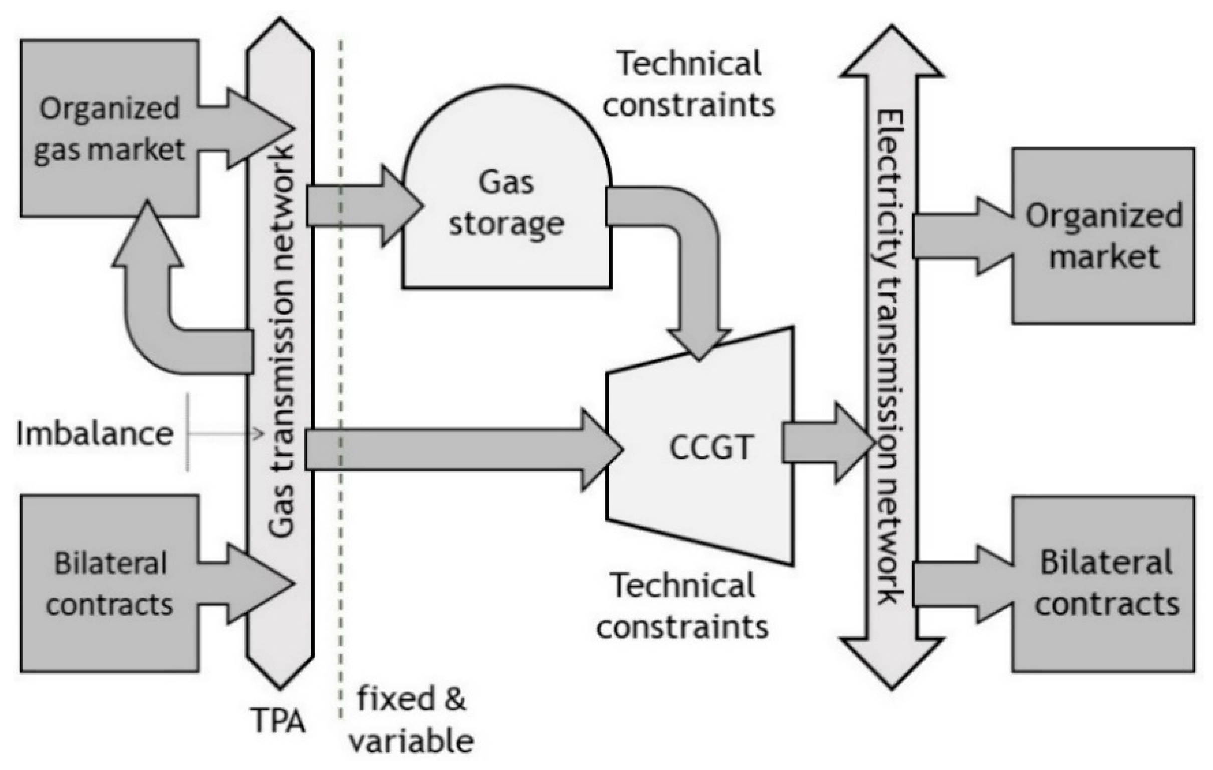
2.1. Electricity and Gas Markets
- (a)
- Electricity markets: It is assumed that the power producer can participate in two different markets:
- Spot market: This is an organized market where the power producer submits sale hourly bids for the day-ahead energy market. The bids are made for each hour of the next day, and hourly prices result from clearing the market.
- Bilateral contracting in over-the-counter market (OTC). The terms of these contracts are nonprefixed and they are agreed between the signing parties. These contracts are usually middle-term contracts, where the power producer sells hourly quantities of electricity at known prices. Observe that the decisions on bilateral contracting are made before knowing the spot market prices.
- (b)
- Gas markets: the different markets where a producer owning a CCGT must participate in order to obtain gas supply are the following ones:
- Spot market: This is an organized market with auctions and continuous sessions. The power producer may purchase natural gas in products with daily quantities and prices. The daily quantities are usually known and fixed, whereas prices are unknown.
- Bilateral contracting in OTC: Like in the case of electricity bilateral contracts, the terms of these contracts are agreed between the signing parties. We consider middle-term contracts where the power producer purchases natural gas with daily quantities and prices, being that information is known when the contract is signed.
- TPA market: This is an organized market where the power producer acquires firm capacity to withdraw natural gas from the virtual balancing point (VBP) to the CCGT. The VBP is a nonphysical hub that is defined for trading gas in the different markets. The capacity is bought in the TPA market through standard products with regulated daily prices. The capacity tariff is composed of fixed and variable terms known for the power producer.
- Imbalance settlement in the VBP market: This is an organized market where the power producer pays for daily pipeline balancing actions because of differences between initial inventory, injections, trading transactions, and withdrawals. The tariff is composed of a variable term that is known for the power producer.
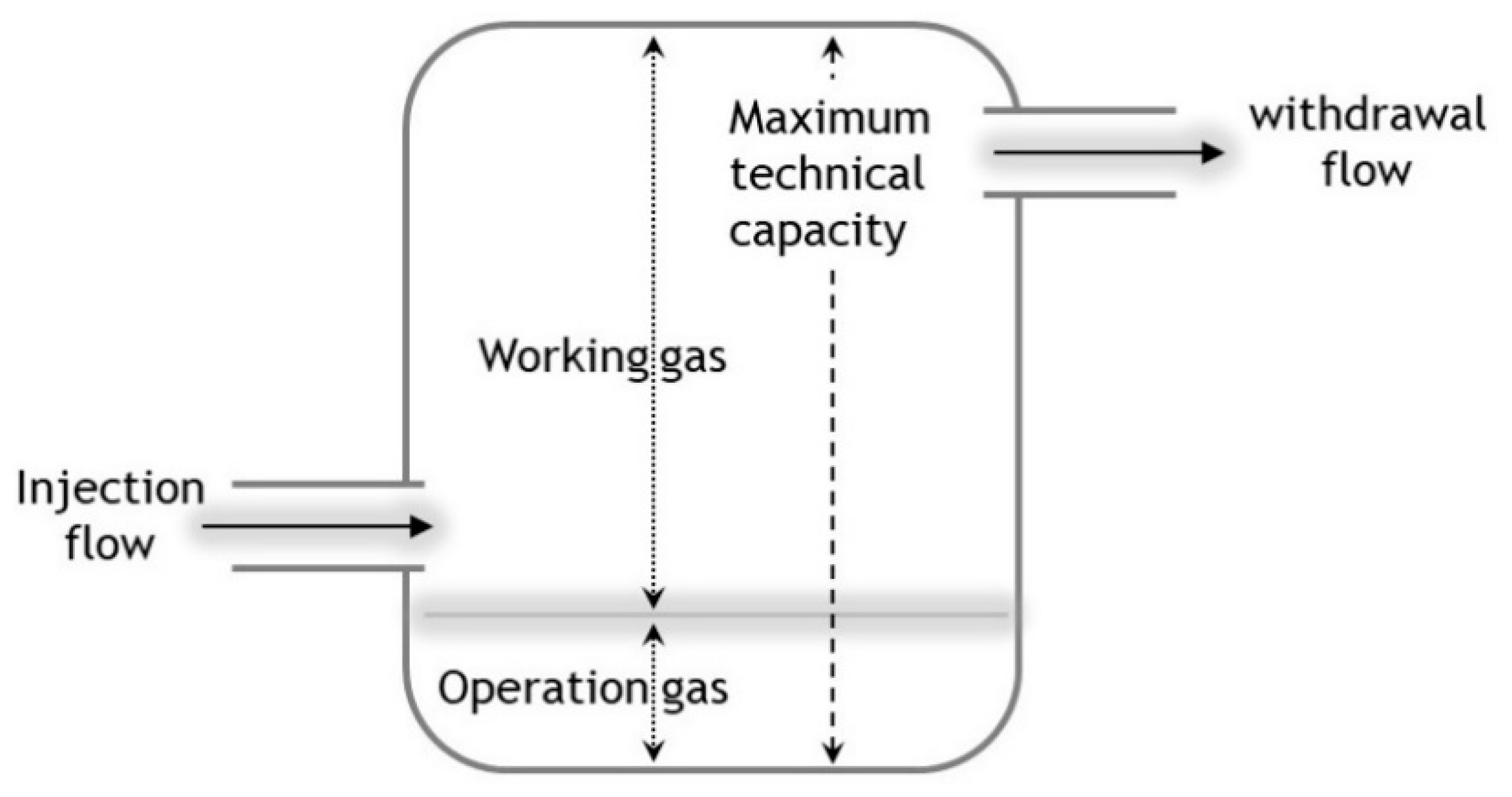
2.2. Gas Storage Unit
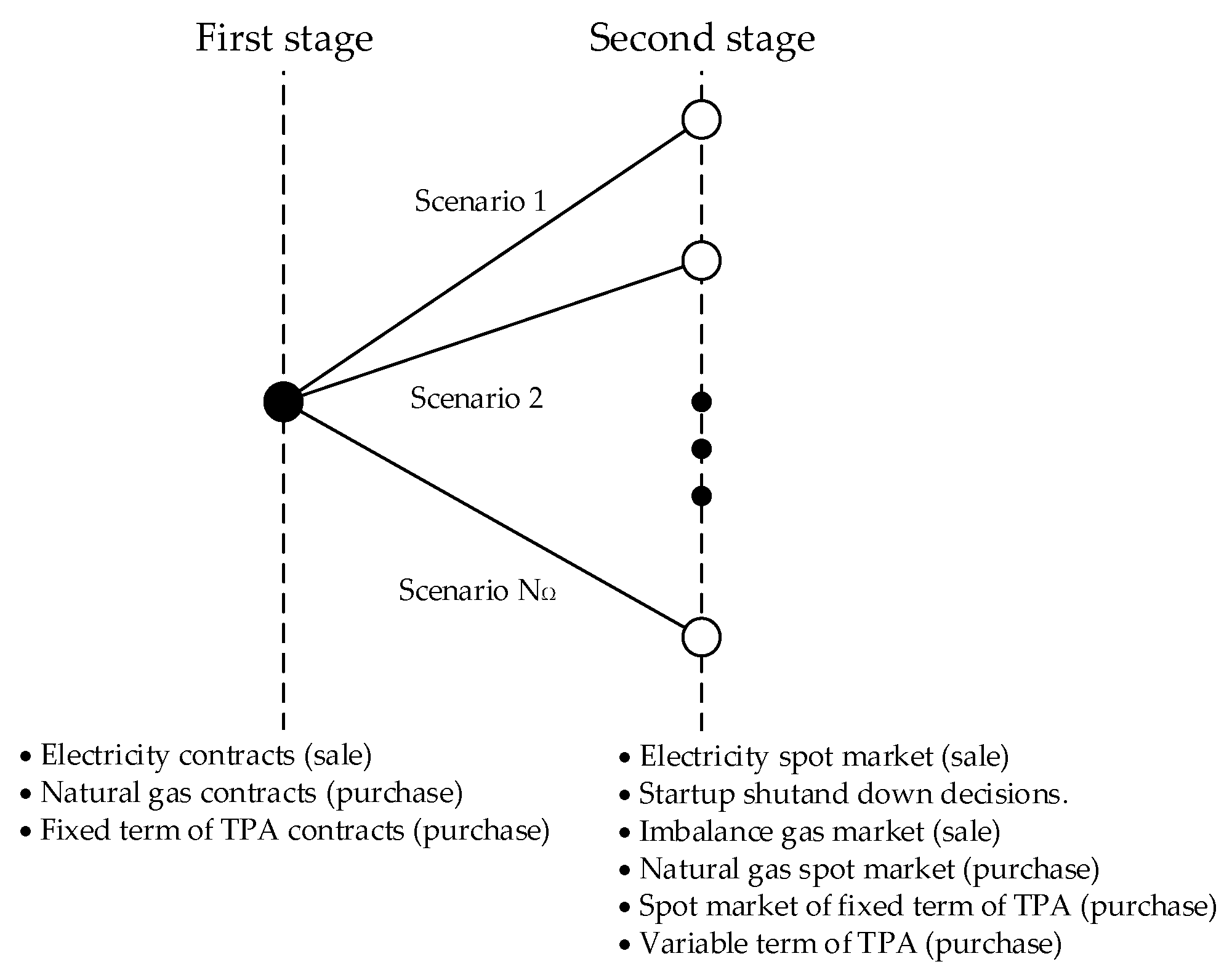
2.3. Decision Making and Uncertainty Characterization
- First-stage decisions:
- Electricity sales in a portfolio of physical bilateral contracts.
- Natural gas purchases in a portfolio of physical bilateral contracts.
- Purchases of the fixed term of TPA for gas capacity through bilateral contracts. The gas capacity purchased from bilateral contracts do not include a premium.
- Second-stage decisions:
- Electricity sales in the spot market.
- Startup and shutdown decisions.
- Sales of the imbalance gas resulting from the day before.
- Natural gas purchases in the spot market.
- Purchases of the fixed term of TPA for gas capacity in the spot market. In this case, the capacity is acquired in auctions of short-term products and these include the premium per product.
- Purchases of the variable term of TPA for gas capacity. This term includes: (i) the gas injected into the storage, (ii) the gas purchased through bilateral contracts, (iii) the gas purchased in the spot market, and (iv) the gas from imbalances and used in the CCGT.
3. Mathematical Formulation
- -
- The objective Equation (1) is equal to the expected profit of the power producer and comprises the following terms:
- -
- The revenue obtained from selling electricity in the bilateral contracting market.
- -
- The expected revenue obtained from selling electricity in the electricity spot market.
- -
- The expected costs derived from startups and shutdowns of the CCGT.
- -
- The cost derived from purchasing gas in the bilateral contracting market.
- -
- The expected revenue obtained from selling gas in the spot market.
- -
- The expected cost derived from purchasing gas in the spot market.
- -
- The expected cost derived from the fixed term of the capacity bought in the TPA market.
- -
- The expected cost derived from the variable term of the capacity bought in the TPA market.
- -
- The expected cost derived from the imbalances of gas in the VBP.
4. Case Study
4.1. Input Data
4.1.1. Combined Cycle Gas Turbine
4.1.2. Natural Gas Storage
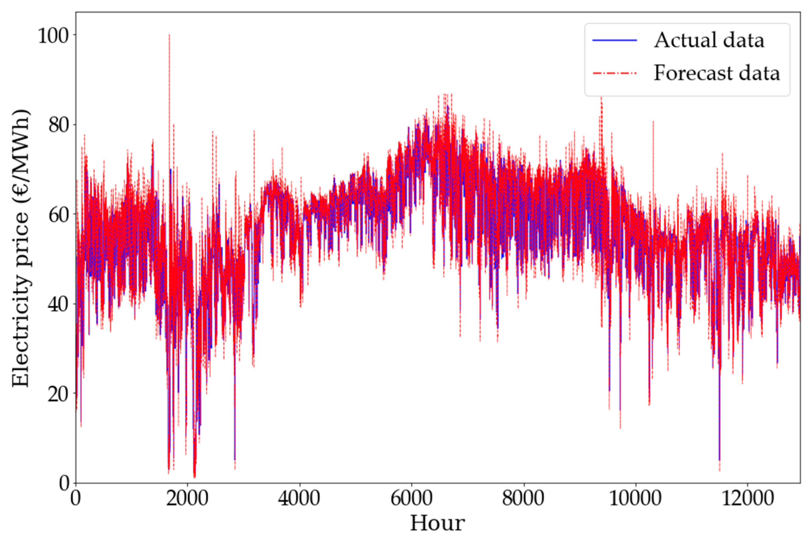
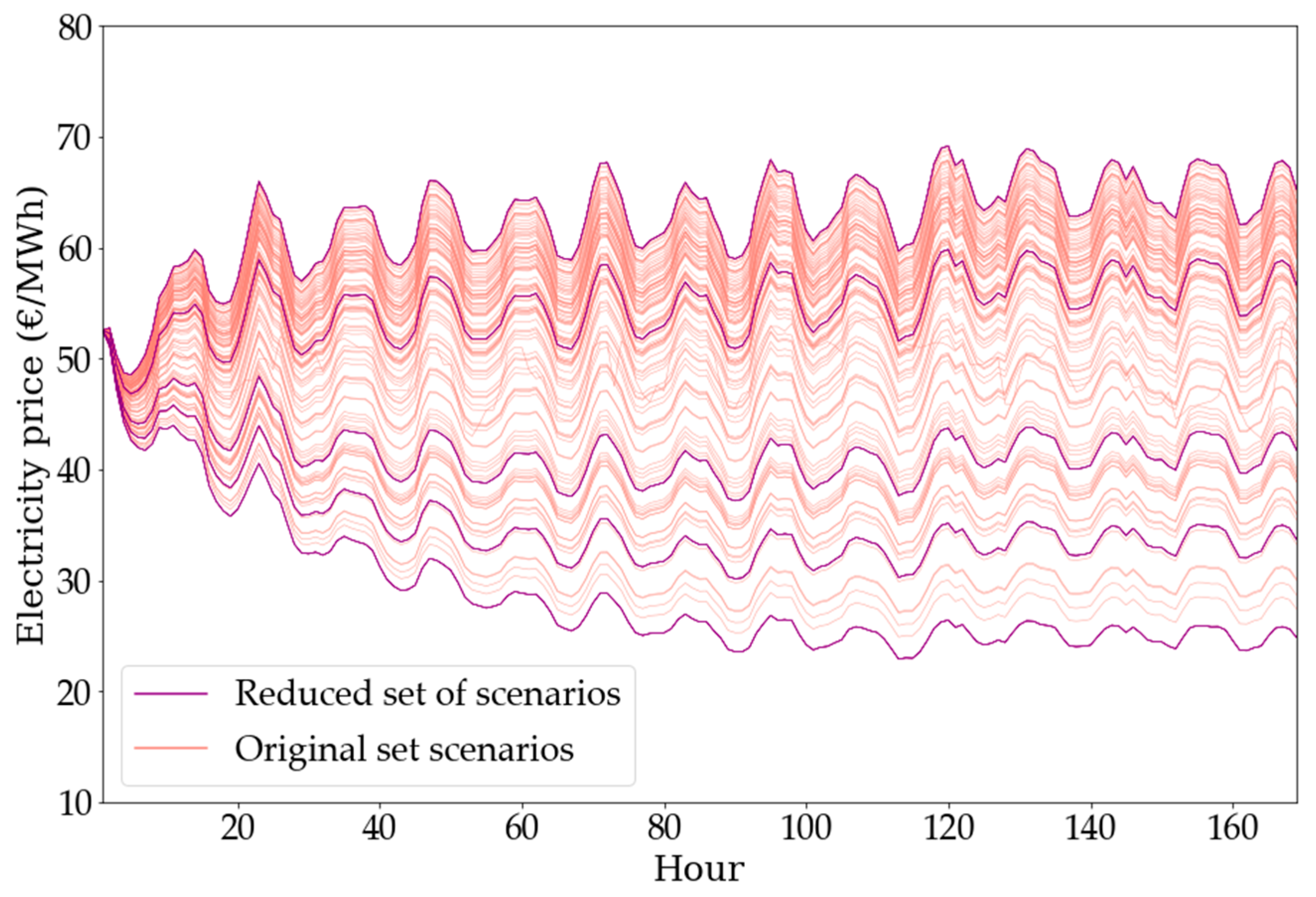
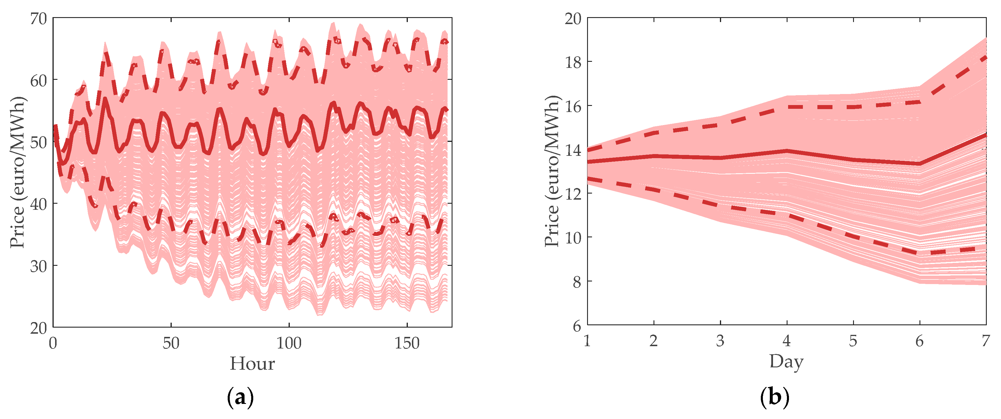
4.1.3. Electricity Contracts and Spot Prices
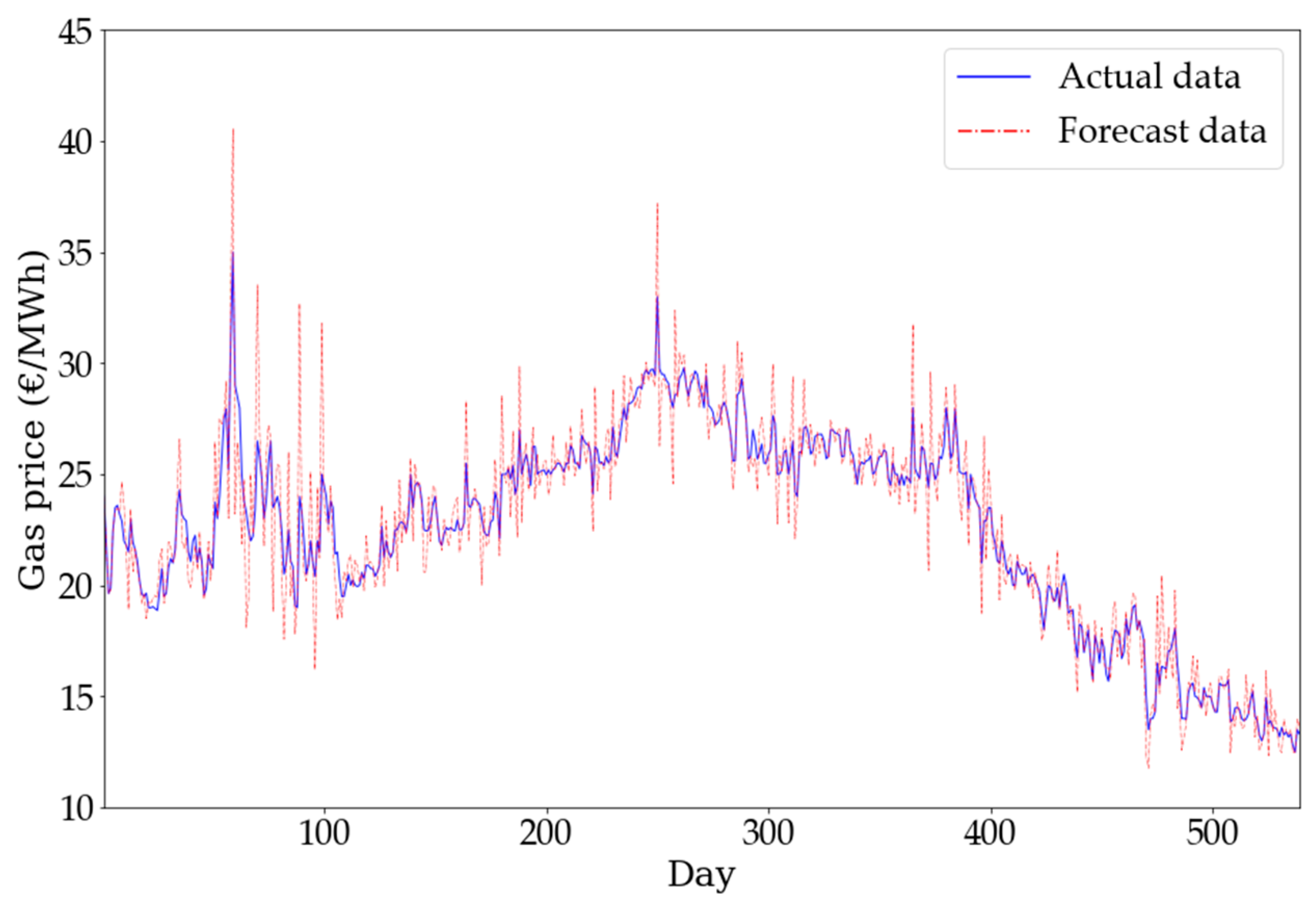
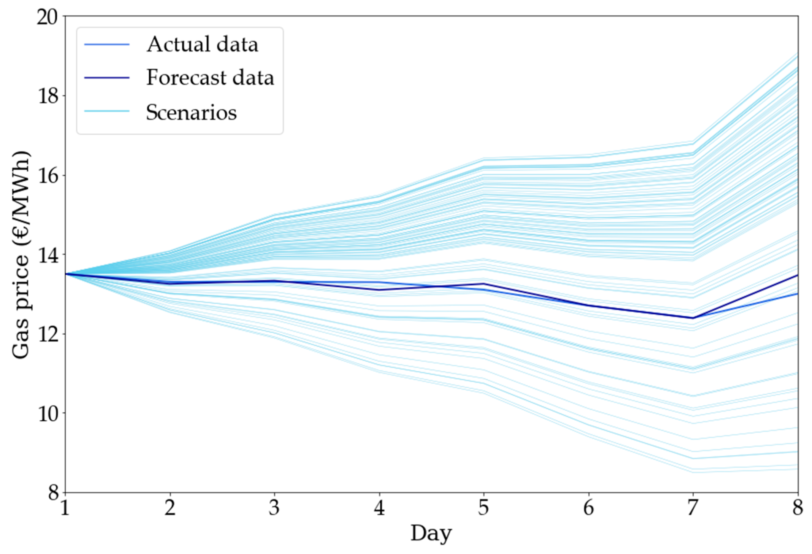
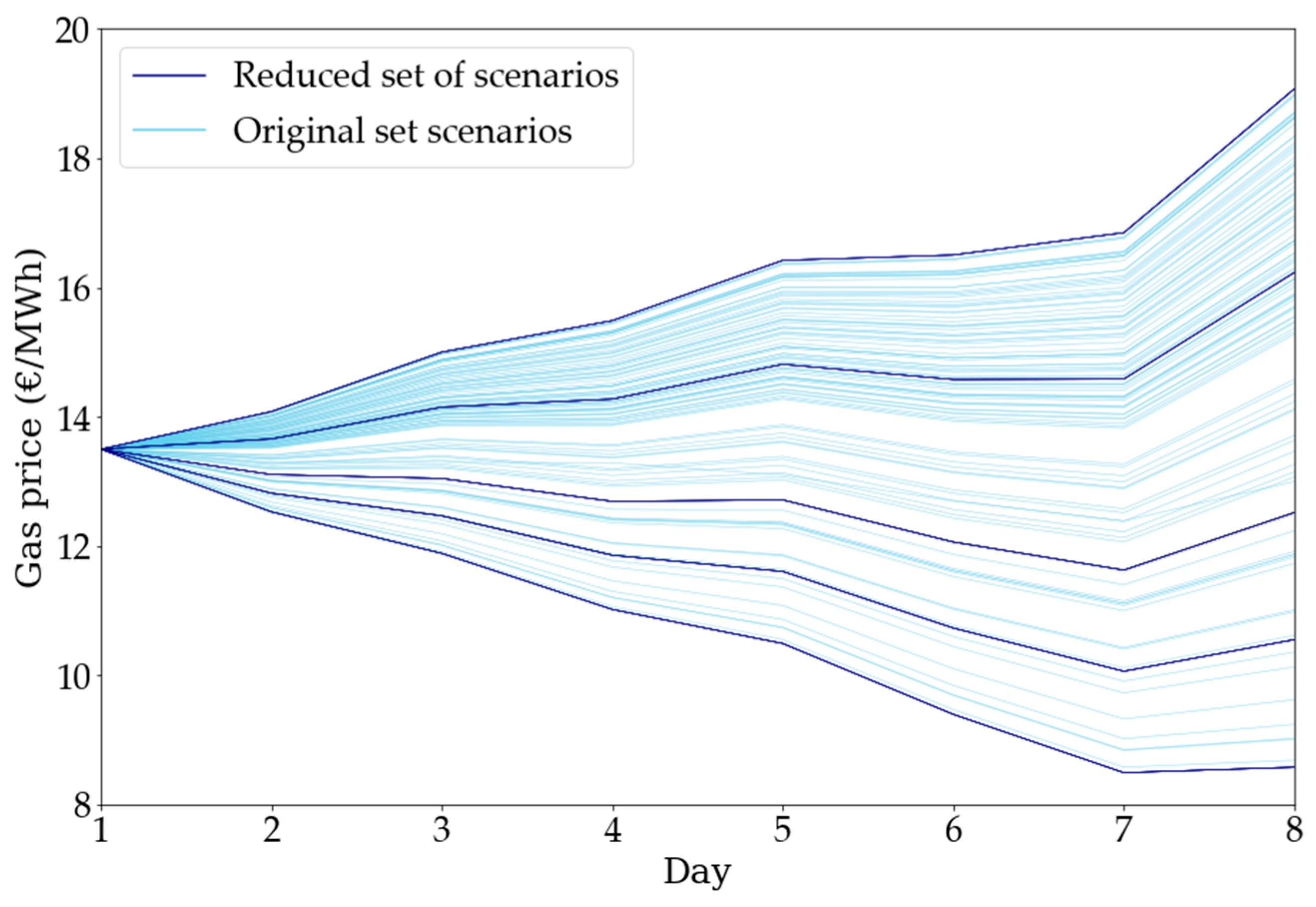
4.1.4. Gas Contracts and Spot Prices
5. Results
5.1. Expected Profit
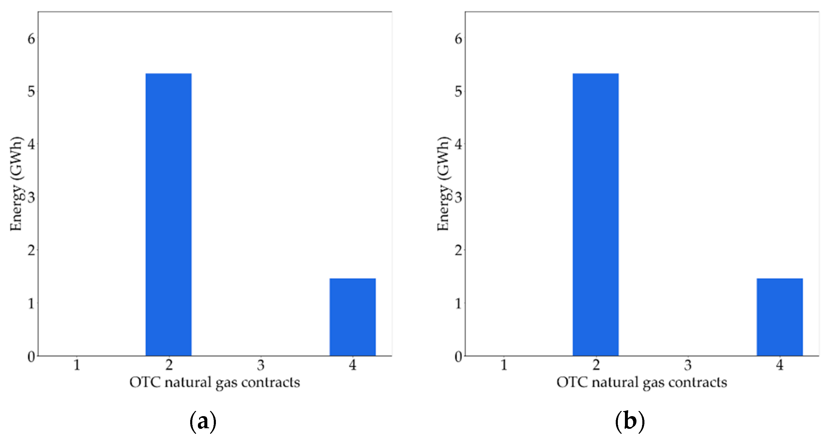
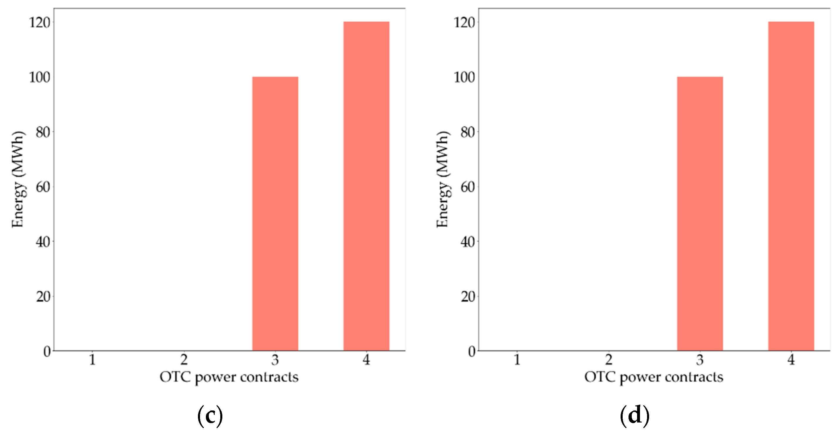
5.2. Bilateral Contracts
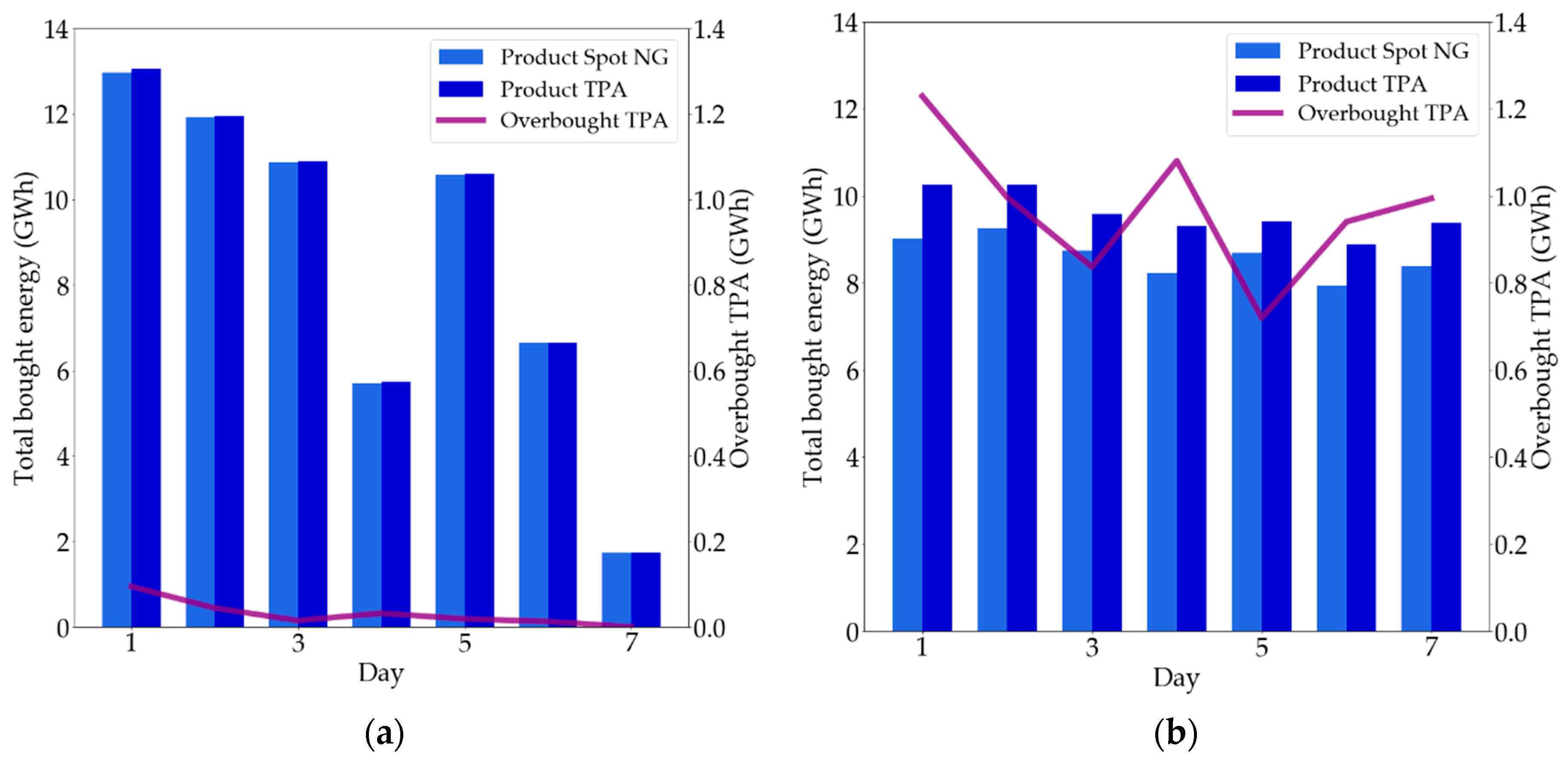
5.3. TPA Contracts
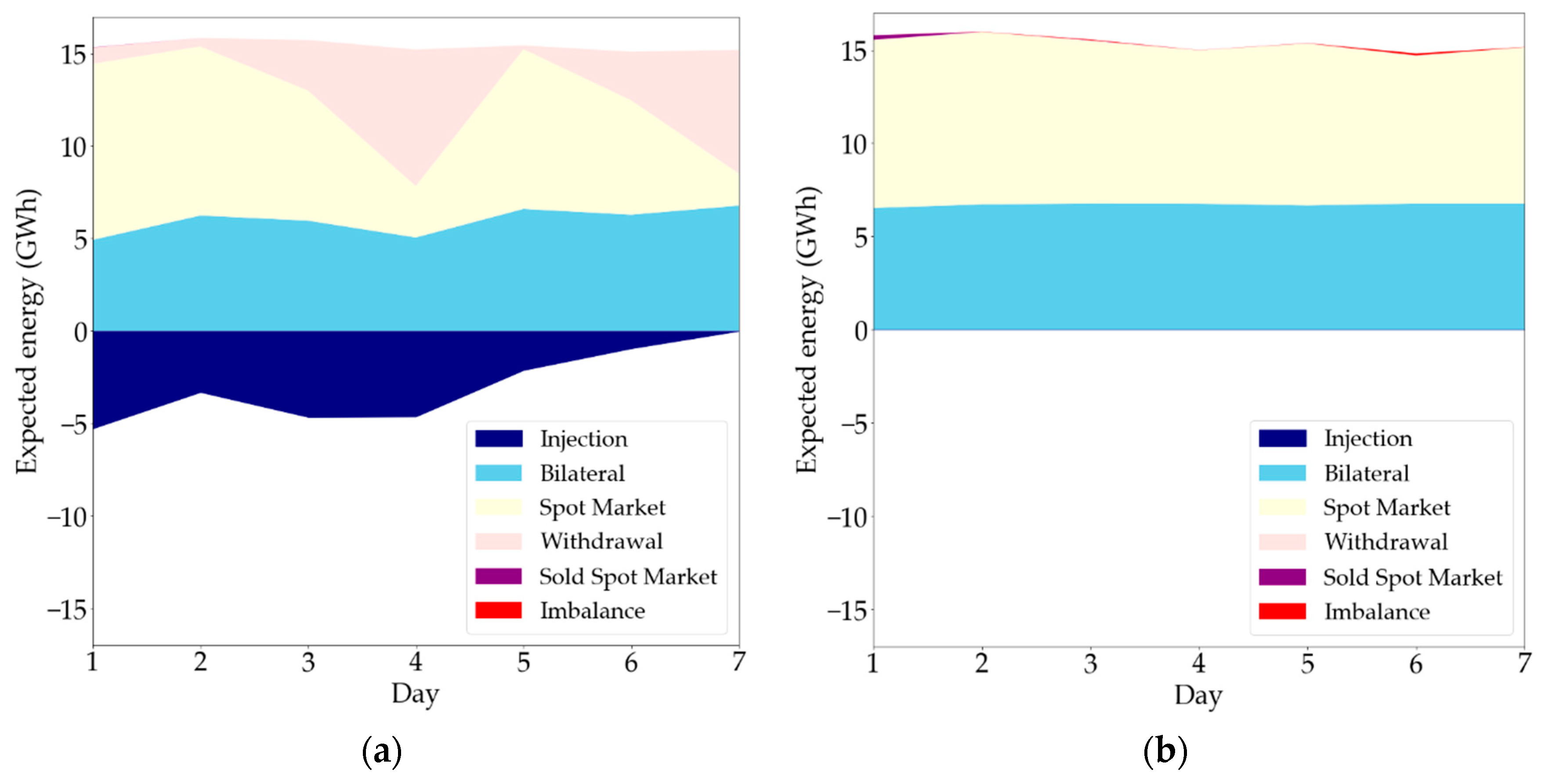
5.4. Expected Gas Procurement
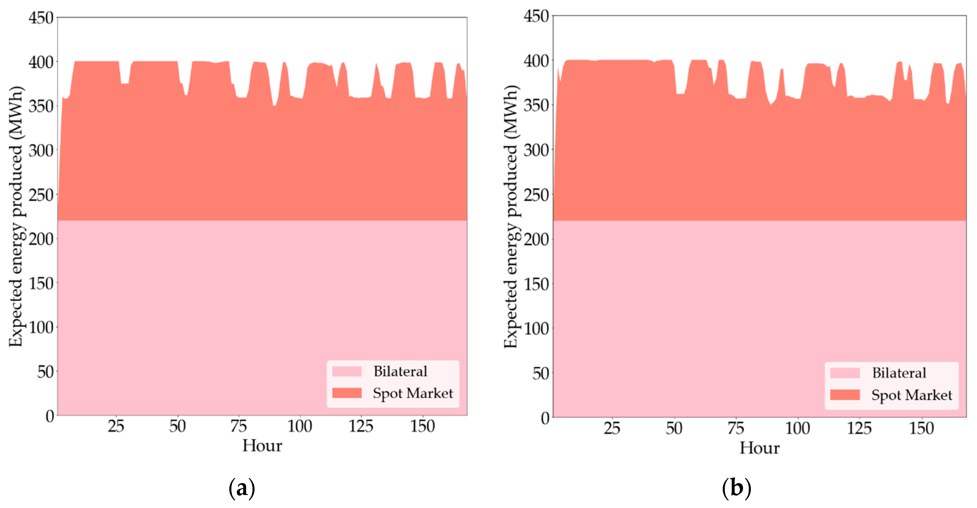
5.5. Expected Electricity Sales
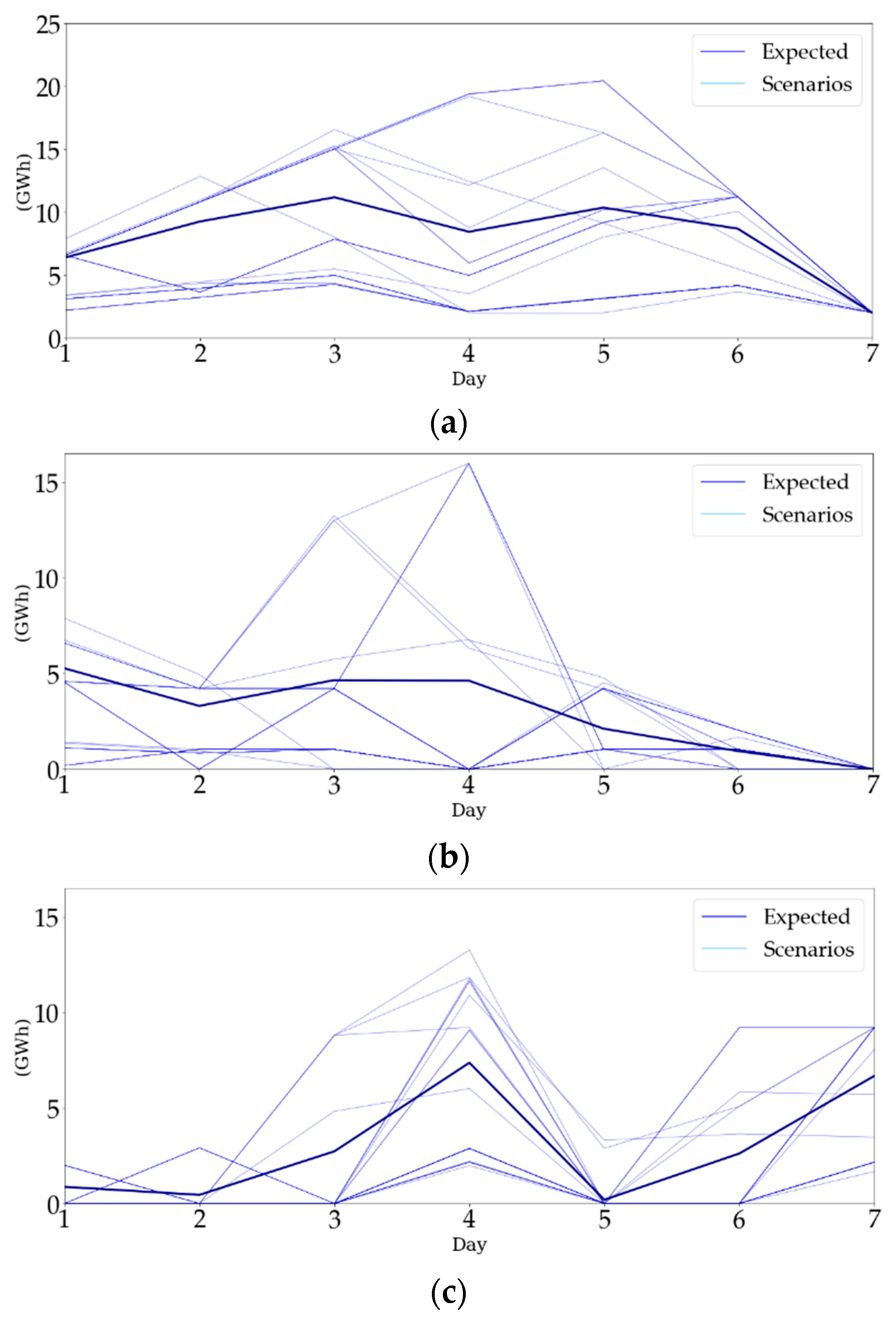
5.6. Storage Operation Per Scenario
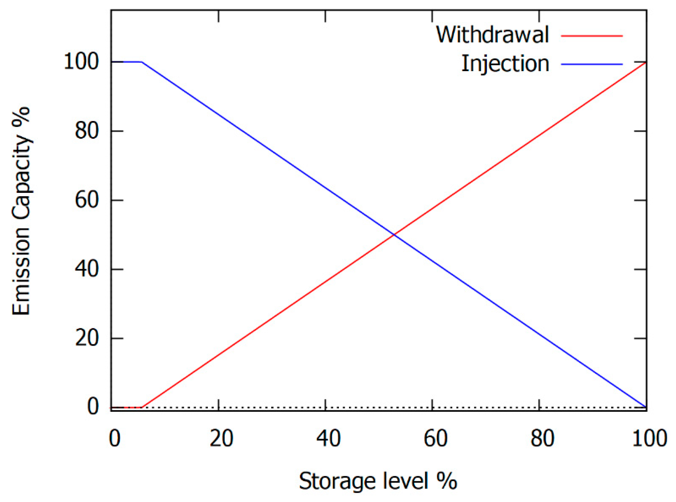
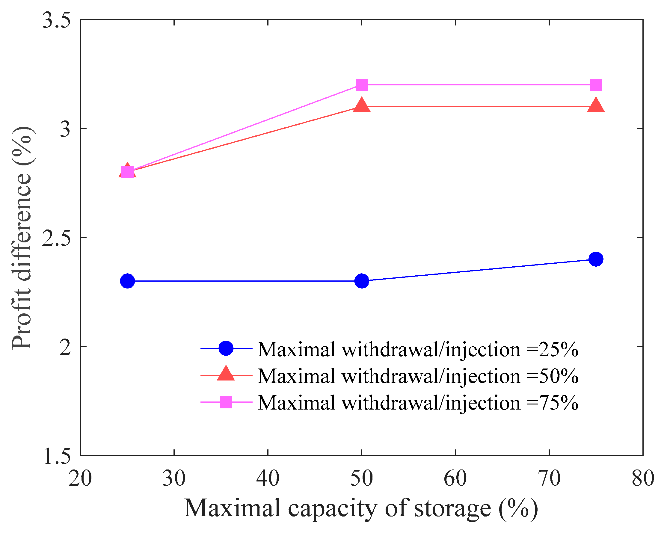
5.7. Sensitivity Analysis: Gas Storage Unit
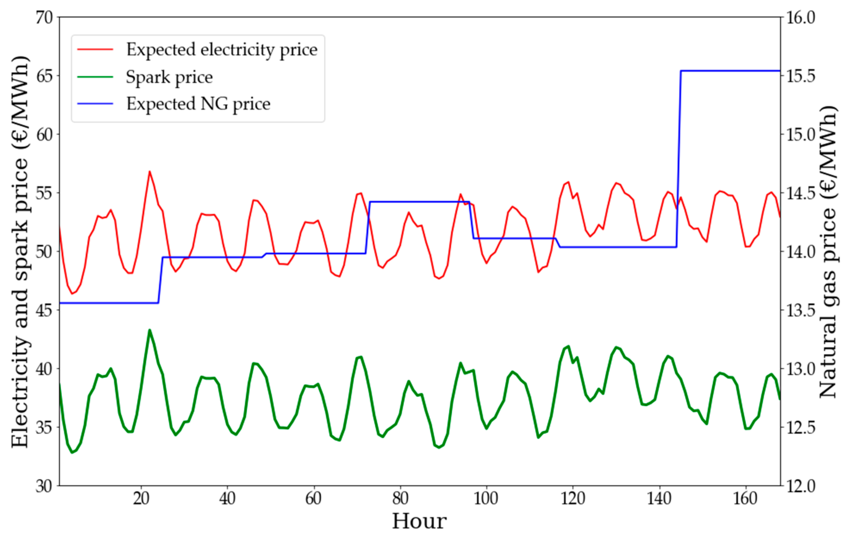
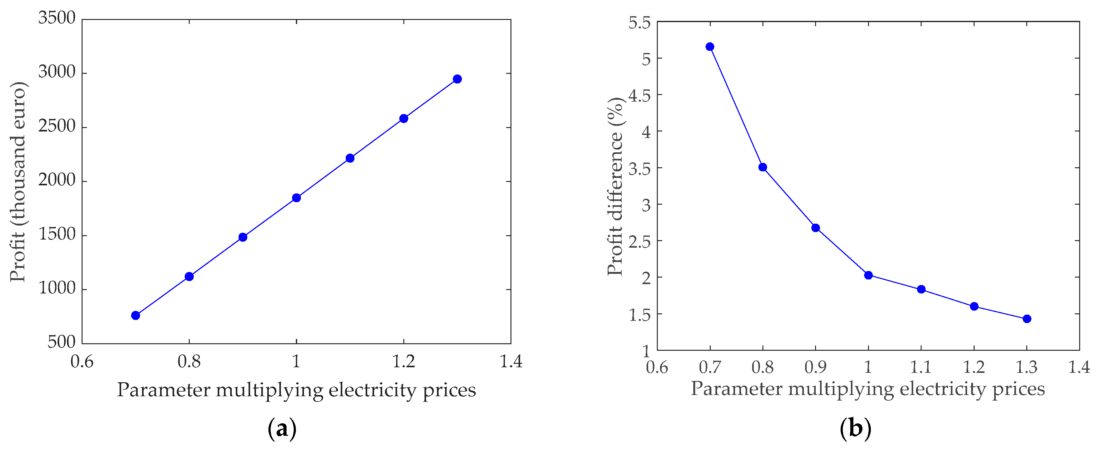
5.8. Sensitivity Analysis: Spark Price
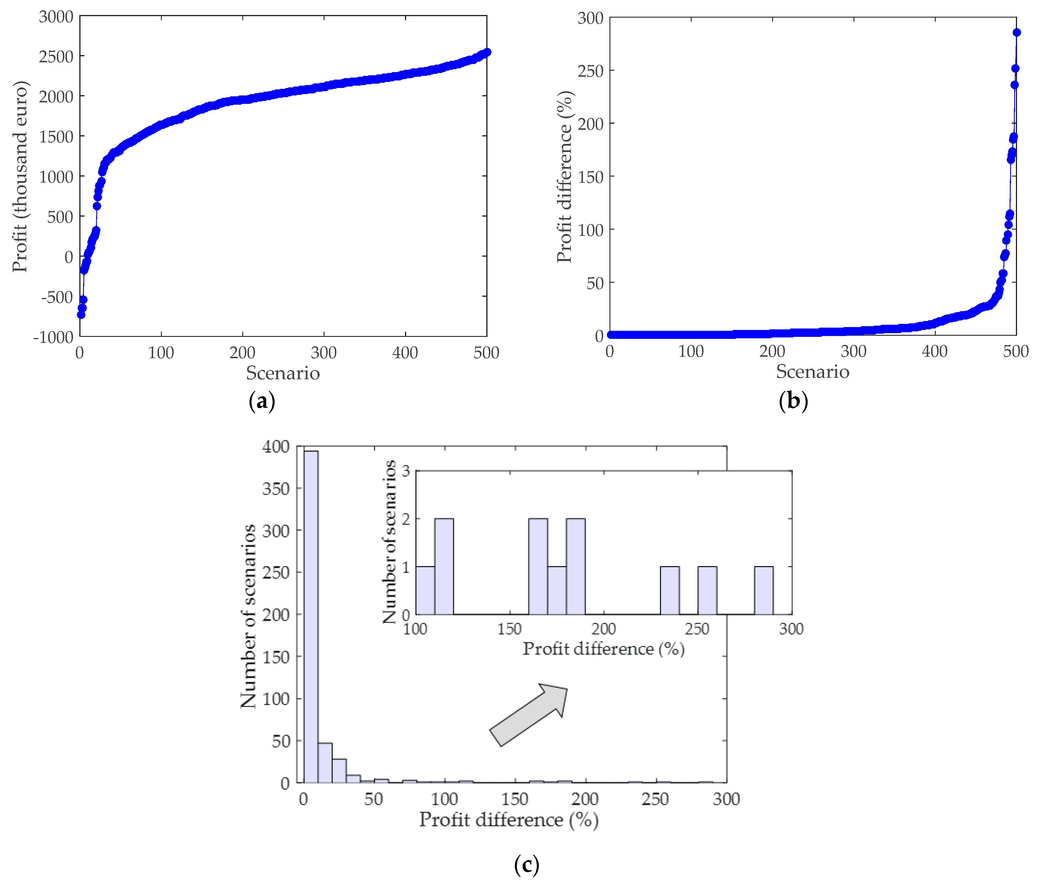
5.9. Out-of-Sample Analysis
6. Conclusions
Author Contributions
Funding
Acknowledgments
Conflicts of Interest
Appendix A
| ARIMA | Autoregressive integrated moving average model |
| CCGT | Combined-cycle gas turbine |
| LHV | Lower heating value |
| LMP | Locational marginal prices |
| LNG | Liquified natural gas |
| NG | Natural gas |
| OTC | Over the counter |
| PGE2 | PG&E Citygate hub prices used in CAISO market systems |
| SARIMA | Seasonal autoregressive integrated moving average model |
| TPA | Third-party access |
| VBP | Virtual balancing point |
| Index of breakpoints used to model the piecewise linear approximation of the gas consumption of the CCGT | |
| Index of time periods [daily] | |
| Index of natural gas products | |
| Index of time periods [hourly] | |
| Index of TPA products | |
| Index of natural gas bilateral contracts | |
| Index of electricity bilateral contracts | |
| Index of scenarios |
| Set of breakpoints “Heat rate blocks” | |
| Set of electricity bilateral contracts | |
| Set of daily time periods | |
| Set of natural gas products | |
| Set of hourly time periods | |
| Set establishing relation between daily and hourly periods | |
| Set of TPA products | |
| Set of natural gas bilateral contracts | |
| Set of natural gas bilateral contracts defined in day d | |
| Set of natural electricity bilateral contracts | |
| Set of natural electricity bilateral contracts in hourly period k | |
| Set of scenarios |
| Binary variable that is equal to 1 if electricity bilateral contract z is signed, being 0 otherwise | |
| Binary variable that is equal to 1 if gas bilateral contract y is signed, being 0 otherwise | |
| Shutdown cost in hourly period k and scenario ω | |
| Startup cost in hourly period k and scenario ω | |
| Binary variable that is equal to 1 if gas product h is bought in daily period d and scenario ω, being 0 otherwise | |
| Binary variable that is equal to 1 if TPA product t is bought in daily period d and scenario ω, being 0 otherwise | |
| Power generated in hourly period k and scenario ω | |
| Power sold in spot market in hourly period k and scenario ω | |
| Power produced in hourly period k in breakpoint b and scenario ω | |
| Gas quantity consumed in hourly period k and scenario ω | |
| Gas quantity stored at the end of the daily period d in the storage in scenario ω | |
| Imbalance gas quantity in PVB at the end of the daily period d and scenario ω | |
| Gas quantity injected in daily period d in the storage in scenario ω | |
| Gas quantity bought in spot market in daily period d in product h and scenario ω | |
| TPA capacity bought in daily period d in product t and scenario ω | |
| Gas quantity withdrawn in daily period d from the storage in scenario ω | |
| Bilateral contracts gas quantity consumed in daily period d and scenario ω | |
| Imbalance gas quantity consumed in daily period d and scenario ω | |
| Gas quantity bought in spot market and consumed in daily period d and scenario ω | |
| Imbalance quantity by gas overbought in bilateral contracts in daily period d and scenario ω | |
| Imbalance gas quantity from the day before and not completely consumed in daily period d and scenario ω | |
| Imbalance quantity by gas overbought in spot market in daily period d and scenario ω | |
| Bilateral contracts gas quantity stored in daily period d in the storage in scenario ω | |
| Imbalance gas quantity injected in daily period d in the storage in scenario ω | |
| Gas quantity bought in spot market in daily period d injected in the storage in scenario ω | |
| Gas quantity sold in continuous session in daily period d and scenario ω | |
| Binary variable that is equal to 1 if the status of the CCGT unit is online in hourly period k and scenario ω, being 0 otherwise | |
| Binary variable that is equal to 1 if the level of gas in the storage is higher than the operation gas in daily period d and scenario ω, being 0 otherwise |
| Shutdown cost of CCGT unit | |
| Startup cost of CCGT unit | |
| Number of breakpoints “Heat rate blocks” | |
| Number of electricity bilateral contracts | |
| Number of daily time periods | |
| Number of gas products | |
| Number of hourly time periods | |
| Number of TPA products | |
| Number of gas bilateral contracts | |
| Number of scenarios | |
| Initial status of the gas quantity in the storage, being equal to 1 if gas stored is larger than the operation gas | |
| Power sold in bilateral contract z | |
| Maximum nominal power output of CCGT unit | |
| Minimum power output of CCGT unit | |
| Initial power output of CCGT unit | |
| Power output of CCGT unit in breakpoint b | |
| Gas quantity bought in period d in bilateral contract y | |
| Minimum quantity of operation gas in the storage | |
| Maximum technical capacity of the storage | |
| Initial gas quantity stored in the storage | |
| Maximum injection capacity of the storage | |
| Maximum withdrawal capacity of the storage | |
| Gas quantity consumed by CCGT unit working on minimum power output | |
| Initial imbalance in PVB | |
| Gas quantity bid in auctions in daily period d of natural gas product h | |
| TPA Capacity bid in auctions in daily period d of firm exit gas capacity product h | |
| Ramp-down limit of CCGT unit | |
| Ramp-up limit of CCGT unit | |
| Heat rate slope of CCGT unit in breakpoint of consumption b | |
| Shutdown ramp limit of CCGT unit | |
| Startup ramp limit of CCGT unit | |
| Initial status of CCGT unit, that is equal to 1 if the unit is online | |
| Fixed term coefficient of TPA capacity in auctions in period d of firm exit gas capacity product t | |
| Fixed term coefficient of TPA capacity in period d of firm exit gas in bilateral contract y | |
| Coefficient that represents an additional cost to sale gas in continuous sessions | |
| Fixed term premium of TPA capacity in auctions in period d of firm exit gas capacity product t | |
| Electricity price in bilateral contract z | |
| Gas price in bilateral contract y | |
| Electricity spot price in hourly period k and scenario ω | |
| Gas price in continuous sessions in daily period d and scenario ω | |
| Gas spot price in auctions in period d of product h and scenario ω | |
| TPA fixed term of the tariff for exit firm capacity in daily period d | |
| TPA variable term of the tariff for exit firm capacity in daily period d | |
| PVB imbalance tariff in daily period d | |
| Scenario probability |
References
- COM 773 Final at EUR-Lex. 2018. Available online: https://eur-lex.europa.eu/homepage.html (accessed on 22 August 2019).
- IEA (International Energy Agency). World Energy Outlook. Available online: https://www.iea.org/reports/world-energy-outlook-2018 (accessed on 1 September 2019).
- Gas for Climate. The Optimal Role for Gas in a Net-Zero Emissions Energy System at Navigant. Available online: https://www.navigant.com/ (accessed on 22 August 2019).
- Kaye, R.J.; Outhred, H.R.; Bannister, C.H. Forward contracts for the operation of an electricity industry under spot pricing. IEEE Trans. Power Syst. 1990, 5, 46–52. [Google Scholar] [CrossRef]
- Gómez-Expósito, A.; Conejo, A.J.; Canizares, C. Electric Energy Systems: Analysis and Operation; CRC Press: Boca Raton, FL, USA, 2008. [Google Scholar]
- Shahidehpour, M.; Yamin, H.; Li, Z. Market Overview in Electric Power Systems; John Wiley & Sons, Inc: New York, NY, USA, 2002. [Google Scholar]
- Jirutitijaroen, P.; Kim, S.; Kittithreerapronchai, O.; Prina, J. An optimization model for natural gas supply portfolios of a power generation company. Appl. Energy 2013, 107, 1–9. [Google Scholar] [CrossRef]
- Zhuang, D.X.; Jiang, J.N.; Gan, D. Optimal short-term natural gas nomination decision in generation portfolio management. Eur. Trans. Electr. Power 2011, 21, 1–10. [Google Scholar] [CrossRef]
- Chen, H.; Baldick, R. Optimizing short-term natural gas supply portfolio for electric utility companies. IEEE Trans. Power Syst. 2007, 22, 232–239. [Google Scholar] [CrossRef]
- Dueñas, P.; Barquín, J.; Reneses, J. Strategic management of multi-year natural gas contracts in electricity markets. IEEE Trans. Power Syst. 2012, 27, 771–779. [Google Scholar] [CrossRef]
- Knudsen, B.R.; Whitson, C.H.; Foss, B. Shale-gas scheduling for natural-gas supply in electric power production. Energy 2014, 78, 165–182. [Google Scholar] [CrossRef]
- Ansary, M.; Latify, M.A.; Yousefy, G.R. GenCo’s mid-term optimal operation analysis: Interaction of wind farm, gas turbine, and energy storage systems in electricity and natural gas markets. IET Gener. Transm. Distrib. 2019, 13, 2328–2338. [Google Scholar] [CrossRef]
- Midthun, K.T. Optimization Models for Liberalized Natural Gas Markets. Fakultet for Samfunnsvitenskap og Teknologiledelse. Ph.D. Dissertation. 2007. Available online: https://ntnuopen.ntnu.no/ntnu-xmlui/handle/11250/265615 (accessed on 1 September 2019).
- Gabriel, S.A.; Kiet, S.; Zhuang, J. A mixed complementarity-based equilibrium model of natural gas markets. Oper. Res. 2005, 53, 799–818. [Google Scholar] [CrossRef]
- Holland, A. Injection/withdrawal scheduling for natural gas storage facilities. In Proceedings of the 2007 ACM Symposium on Applied Computing, Seoul, Korea, 11–15 March 2007; pp. 332–333. Available online: https://www.academia.edu/2811831/Injection_withdrawal_scheduling_for_natural_gas_storage_facilities (accessed on 1 September 2019).
- Birge, J.R.; Louveaux, F. Introduction to Stochastic Programming, Second Edition; Springer: New York, NY, USA, 2011. [Google Scholar]
- Kall, P.; Wallace, S.W.; Kall, P. Stochastic Programming; Wiley: Chichester, UK, 1994. [Google Scholar]
- Wallace, S.W.; Ziemba, W.T. (Eds.) Applications of Stochastic Programming; SIAM-MPS: Philadelphia, PA, USA, 2005. [Google Scholar]
- Conejo, A.J.; Carrión, M.; Morales, J.M. Decision Making under Uncertainty in Electricity Markets; Springer: New York, NY, USA, 2010. [Google Scholar]
- OMIE. Available online: http://www.omie.es/files/flash/ResultadosMercado.html# (accessed on 20 November 2019).
- Dupačová, J.; Gröwe-Kuska, N.; Römisch, W. Scenario reduction in stochastic programming. Math. Progr. 2003, 95, 493–511. [Google Scholar] [CrossRef]
- Box, G.E.P.; Jenkins, G.M.; Reinsel, G.C. Time Series Analysis: Forecasting and Control, 5th ed.; Wiley: Upper Saddle River, NJ, USA, 2015. [Google Scholar]
- Matlab. Available online: https://www.mathworks.com/products/matlab.html (accessed on 20 November 2019).
- MIBGAS. Available online: http://www.mibgas.es/en/gas-markets (accessed on 22 August 2019).
- BOE. Available online: https://www.boe.es/buscar/index.php?lang=en (accessed on 21 November 2019).
- CPLEX 12 at GAMS. Available online: https://www.gams.com/latest/docs/S_CPLEX.html (accessed on 22 August 2019).
- GAMS. Available online: https://www.gams.com (accessed on 22 August 2019).


| Breakpoint | Heat Rate Slope | Power Output (MWh) | Gas Consumption (MWh) |
|---|---|---|---|
| Minimum 1 | - | 120.00 | 267.95 |
| 1 | 1.39 | 280.00 | 489.87 |
| 2 | 1.45 | 360.00 | 605.87 |
| 3 | 1.52 | 400.00 | 666.51 |
| Bilateral Contract | Energy Sold (MWh) | Prices (€/MWh) |
|---|---|---|
| 1 | 20.00 | 38.35 |
| 2 | 40.00 | 42.78 |
| 3 | 100.00 | 55.00 |
| 4 | 120.00 | 59.21 |
| Coefficient | |||
|---|---|---|---|
| Nonseasonal | Seasonal | ||
| 0.953392686 | −0.689749350 | ||
| −0.537356443 | |||
| Constant K | 0.0000814540 | −0.307308537 | |
| −0.154635954 | |||
| Number of Scenarios | Electricity Spot Prices (euro/MWh) | ||
|---|---|---|---|
| Perc. 10% | Perc. 50% | Perc. 90% | |
| 100 | 37.34 | 54.73 | 61.17 |
| 80 | 37.36 | 54.73 | 61.17 |
| 60 | 37.36 | 54.79 | 61.17 |
| 40 | 37.11 | 54.79 | 61.17 |
| 20 | 35.13 | 54.79 | 60.76 |
| 10 | 35.13 | 54.79 | 62.66 |
| 5 | 35.12 | 54.79 | 62.66 |
| 3 | 41.70 | 54.79 | 54.79 |
| 1 | 54.79 | 54.79 | 54.79 |
| Scenario | Probability | Average Price (€/MWh) |
|---|---|---|
| 1 | 0.44 | 54.79 |
| 2 | 0.03 | 28.85 |
| 3 | 0.19 | 41.70 |
| 4 | 0.25 | 62.66 |
| 5 | 0.09 | 35.13 |
| Bilateral Contract | Quantity Purchased (MWh/day) | Prices (€/MWh) |
|---|---|---|
| 1 | 6430.80 | 15.23 |
| 2 | 5326.08 | 12.39 |
| 3 | 2784.00 | 14.85 |
| 4 | 1455.36 | 13.50 |
| Product | Quantity (MWh/day) |
|---|---|
| 1 | 130 |
| 2 | 1000 |
| 3 | 2000 |
| 4 | 2100 |
| 5 | 3200 |
| 6 | 4000 |
| 7 | 5200 |
| 8 | 7050 |
| Total per day | 24,680 |
| Coefficient | |||
|---|---|---|---|
| Nonseasonal | Seasonal | ||
| 0.000000000 | 0.119851759 | ||
| −0.095659720 | −0.003820293 | ||
| Constant K | −0.000010676 | ||
| Number of Scenarios | Gas Spot Prices (euro/MWh) | ||
|---|---|---|---|
| Perc. 10% | Perc. 50% | Perc. 90% | |
| 100 | 11.58 | 14.59 | 15.95 |
| 80 | 11.58 | 14.58 | 15.95 |
| 60 | 11.59 | 14.58 | 15.95 |
| 40 | 11.57 | 14.61 | 15.95 |
| 20 | 11.57 | 14.61 | 16.00 |
| 10 | 11.44 | 14.61 | 16.20 |
| 5 | 11.44 | 14.61 | 16.20 |
| 3 | 12.55 | 14.61 | 14.61 |
| 1 | 14.61 | 14.61 | 14.61 |
| Scenario | Probability | Average Price (€/MWh) |
|---|---|---|
| 1 | 0.48 | 14.65 |
| 2 | 0.05 | 10.34 |
| 3 | 0.16 | 12.53 |
| 4 | 0.24 | 16.20 |
| 5 | 0.07 | 11.44 |
| Product | Type | Day 1 | Day 2 | Day 3 | Day 4 | Day 5 | Day 6 | Day 7 |
|---|---|---|---|---|---|---|---|---|
| 1 | Monthly | 1.00 | 1.00 | 1.00 | 1.00 | 1.00 | 1.20 | 1.20 |
| 2 | Monthly | 1.00 | 1.00 | 1.00 | 1.00 | 1.00 | 1.20 | 1.20 |
| 3 | Daily | 0.08 | 0.08 | 0.08 | 0.08 | 0.08 | 0.08 | 0.08 |
| 4 | Monthly | 1.00 | 1.00 | 1.00 | 1.00 | 1.00 | 1.20 | 1.20 |
| 5 | Quarterly | 1.21 | 1.21 | 1.21 | 1.21 | 1.21 | 1.08 | 1.08 |
| 6 | Quarterly | 1.21 | 1.21 | 1.21 | 1.21 | 1.21 | 1.08 | 1.08 |
| 7 | Daily | 0.08 | 0.08 | 0.08 | 0.08 | 0.08 | 0.08 | 0.08 |
| 8 | Daily | 0.08 | 0.08 | 0.08 | 0.08 | 0.08 | 0.08 | 0.08 |
| Bilateral Contract | Type | Day 1 | Day 2 | Day 3 | Day 4 | Day 5 | Day 6 | Day 7 |
|---|---|---|---|---|---|---|---|---|
| 1 | Monthly | 1.00 | 1.00 | 1.00 | 1.00 | 1.00 | 1.20 | 1.20 |
| 2 | Daily | 0.08 | 0.08 | 0.08 | 0.08 | 0.08 | 0.08 | 0.08 |
| 3 | Monthly | 1.00 | 1.00 | 1.00 | 1.00 | 1.00 | 1.20 | 1.20 |
| 4 | Daily | 0.08 | 0.08 | 0.08 | 0.08 | 0.08 | 0.08 | 0.08 |
| Product | Quantity (GWh/day) | Premium (€/MWh) | ||||||
|---|---|---|---|---|---|---|---|---|
| Day 1 | Day 2 | Day 3 | Day 4 | Day 5 | Day 6 | Day 7 | ||
| 1 | 0.10 | 0.10 | 0.10 | 0.10 | 0.10 | 0.13 | 0.13 | 0.100 |
| 2 | 2.00 | 2.00 | 2.00 | 2.00 | 2.00 | 1.00 | 1.00 | 0.001 |
| 3 | 3.20 | 3.20 | 3.20 | 3.20 | 3.20 | 2.00 | 2.00 | 0.100 |
| 4 | 4.00 | 4.00 | 4.00 | 4.00 | 4.00 | 2,10 | 2,10 | 0.100 |
| 5 | 1.13 | 1.13 | 1.13 | 1.13 | 1.13 | 3.20 | 3.20 | 0.100 |
| 6 | 4.00 | 4.00 | 4.00 | 4.00 | 4.00 | 4.00 | 4.00 | 0.100 |
| 7 | 7.05 | 7.05 | 7.05 | 7.05 | 7.05 | 5.20 | 5.20 | 0.100 |
| 8 | 3.25 | 3.25 | 3.25 | 3.25 | 3.25 | 7.05 | 7.05 | 0.010 |
| Total per day | 24.73 | 24.73 | 24.73 | 24.73 | 24.73 | 24.68 | 24.68 | -- |
| Item | Value |
|---|---|
| binary variables (×103) | 7.183 |
| continuous variables (×103) | 45.984 |
| constraints (×103) | 54.282 |
| Computing time (h) | 2.863 |
| Number of threads | 10 |
| Item | With Storage | Without Storage |
|---|---|---|
| Expected value (k €) | 1849.2 | 1812.3 |
© 2019 by the authors. Licensee MDPI, Basel, Switzerland. This article is an open access article distributed under the terms and conditions of the Creative Commons Attribution (CC BY) license (http://creativecommons.org/licenses/by/4.0/).
Share and Cite
Gómez-Villarreal, H.; Carrión, M.; Domínguez, R. Optimal Management of Combined-Cycle Gas Units with Gas Storage under Uncertainty. Energies 2020, 13, 113. https://doi.org/10.3390/en13010113
Gómez-Villarreal H, Carrión M, Domínguez R. Optimal Management of Combined-Cycle Gas Units with Gas Storage under Uncertainty. Energies. 2020; 13(1):113. https://doi.org/10.3390/en13010113
Chicago/Turabian StyleGómez-Villarreal, Hernán, Miguel Carrión, and Ruth Domínguez. 2020. "Optimal Management of Combined-Cycle Gas Units with Gas Storage under Uncertainty" Energies 13, no. 1: 113. https://doi.org/10.3390/en13010113
APA StyleGómez-Villarreal, H., Carrión, M., & Domínguez, R. (2020). Optimal Management of Combined-Cycle Gas Units with Gas Storage under Uncertainty. Energies, 13(1), 113. https://doi.org/10.3390/en13010113