Abstract
Within the framework of a Reynolds averaged numerical simulation (RANS) methodology for modeling turbulence, a comparative numerical study of turbulent lifted H2/N2 flames is presented. Three different turbulent combustion models, namely, the eddy dissipation model (EDM), the eddy dissipation concept (EDC), and the composition probability density function (PDF) transport model, are considered in the analysis. A wide range of global and detailed combustion reaction mechanisms are investigated. As turbulence model, the Standard k-ε model is used, which delivered a comparatively good accuracy within an initial validation study, performed for a non-reacting H2/N2 jet. The predictions for the lifted H2/N2 flame are compared with the published measurements of other authors, and the relative performance of the turbulent combustion models and combustion reaction mechanisms are assessed. The flame lift-off height is taken as the measure of prediction quality. The results show that the latter depends remarkably on the reaction mechanism and the turbulent combustion model applied. It is observed that a substantially better prediction quality for the whole range of experimentally observed lift-off heights is provided by the PDF model, when applied in combination with a detailed reaction mechanism dedicated for hydrogen combustion.
1. Introduction
Current power generation techniques by means of thermal machinery [1] are mainly dependent on combustion. As the endeavors for utilizing new energy sources [2] and recovery technologies [3] continue, combustion is prognosed to remain as an important technology for energy conversion, also for the future. It should be noted that combustion plays an important role also for renewable energies, as it is the conversion technology for biomass [4].
Combustion of gases that contain hydrogen [5,6] occupies a significant role for clean and efficient energy supply. Hydrogen allows a useful way of storing the surplus power generated by photovoltaics and wind [7]. Moreover, in place of combustion [8,9], the gasification of waste, biomass, and coal [10,11] provides a useful procedure for efficient and clean conversion, whereby the product synthesis gas (syngas) contains rather considerable portions of hydrogen. Furthermore, there is a developing tendency in hydrogen production using nuclear energy [12]. Obviously, for the environmental aspect, the subsequent combustion of hydrogen is very welcome as it produces no carbon dioxide.
The use of hydrogen-containing gases as fuel in combustion equipment is a considerably demanding task. Hydrogen is very reactive and has quite different material properties in comparison to the gases that are commonly encountered in combustion applications. Thus, it can remarkably affect the properties of the gaseous mixture, even in small amounts. In premixed combustion, a potential complication related with the use of hydrogen blend fuels is the increased tendency of flashback [13]. The counter piece of flashback is blow-off [14]. The predecessor of blow-off is the lift-off that can occur at large jet speed, causing the flame root to leave the burner rim. After the lift-off, depending on the inlet velocity of the jet, a flame stabilized at a distance downstream the rim, i.e., a lifted flame, can be achieved [15].
Computational modeling of turbulent lifted flames that exhibit intricate interactions of turbulence with chemistry [16] is an ambitious undertaking, as the partial premixing occurring at the flame root leads to complex stabilization mechanisms [17].
For modeling the flow turbulence, the large eddy simulation (LES) technique [18,19] is increasingly being applied. However, its application in the industrial development processes is still very challenging because of its high requirements on computational resources. Therefore, the more traditional Reynolds averaged numerical simulation (RANS) approach [20] is still frequently adopted within this context. Given this perspective, the present investigation is focused on the RANS approach for turbulence modeling. Consequently, in the following review, the RANS-based approaches are addressed.
Experimental and numerical investigations of lifted flames of different fuels have been presented by different authors. For clarity, only the hydrogen flames are considered in the following review. One of the early experimental results for lifted hydrogen flames was provided by Cabra et al. [21], who measured a lifted H2/N2 flame in vitiated co-flow. A single flame (with a single co-flow temperature and a single lift-off height) was investigated [21]. Another configuration was experimentally investigated, later on, by Markides and Mastorakos [22]. In Ref. [21], a stable lifted flame was reported, whereas in Ref. [22], different regimes were measured, with emphasis on the unstable regime dominated by auto-ignition. Further experiments on lifted H2/N2 flames were performed by Wu et al. [23] and Gordon et al. [24] in a very similar configuration to that of Ref. [21].
The lifted H2/N2 flame of Cabra et al. [21] was also investigated numerically by the same authors, applying a composition probability density function (PDF) transport model [25] as well as the eddy dissipation concept (EDC) [26] as turbulent combustion models. The GRI-2.1 [27] was used as the detailed reaction mechanism (stripping out the carbon- and nitrogen-containing species and reactions). The overall performance of both of the combustion models were reported to be rather comparable [21]. The measured lift-off height of H/d = 10 (H: Lift-off height, d: Fuel jet diameter) was under-predicted by PDF and EDC as 7 and 8.5, respectively [21]. Later on, the same flame was computationally investigated by many investigators. Masri et al. [28] and Wu et al. [29] calculated the flame [21], adopting a composition PDF transport method as the turbulent combustion model. As reaction mechanism, the mechanisms of Mueller et al. [30] and GRI-2.1 [27] were used. They concluded that even though the mixing rates are still important, the flame is rather controlled by the chemical kinetics. Using the same basic modeling approach (PDF, GRI-2.1) as in Ref. [21], a larger lift-off height, H/d = 8, was predicted, which is closer to the experimental value. The Mueller et al. [30] mechanism led to an over-prediction, with H/d = 14 [28,29].
Lee and Kim [31] investigated the Cabra et al. [21] flame numerically by a direct-quadrature method of moments (DQMOM)-based PDF transport method as the turbulent combustion model, using the reaction mechanism of Mueller et al. [30]. With H/d = 5.7, their results indicated a stronger under-prediction of the lift-off height compared to the previous calculations of other authors [21,28,29]. They achieved a closer prediction (H/d = 9.8) to experiments by reducing the temperature of the co-flowing vitiated gases by 10 K. They justified this modification of the boundary condition with possible turbulent fluctuations of temperature that were not directly captured by the applied RANS approach. A quite similar modeling approach to the previous work [21,28,29] was applied by Mir Najafizadeh et al. [32] using a composition PDF transport turbulent combustion model based on the reaction mechanism of Li et al. [33], which is an updated version of the mechanism of Mueller et al. [30]. In difference to the previously mentioned studies [21,28,29,31], where the Standard k-ε model [20] was used, a Reynolds stress model (RSM) was applied as the turbulence model by Mir Najafizadeh et al. [32]. They could predict a lift-off height close to the experiments [21] by assuming (similar to the Ref. [31]) a lower temperature (by 5 K) for the co-flow, justifying this by the measurement uncertainty.
Mouangue et al. [34] applied Lagrangian intermittent modeling (MIL, Modèle Intermittent Lagrangien) [35] as turbulent combustion model to simulate the flame of Cabra et al. [21], in combination with the GRI-2.1 [27] as the reaction mechanism. Naud et al. [36] analyzed the Cabra et al. [21] flame numerically, using an unsteady flamelet progress variable (UFPV) approach [37] as turbulent combustion model based on the detailed reaction mechanism of Saxena and Williams [38]. As RANS turbulence model, RSM was used. For the experimental conditions, the lift-off height was substantially over-predicted (H/d ≈ 16). A close prediction to the experimental value (H/d = 10, [21]) could be obtained by increasing the co-flow temperature by 8 K and 17 K (depending on the alternative definitions of the progress variable within the UFPV model). The conditional moment closure (CMC) [39] was applied as the turbulent combustion model by De et al. [40] to simulate the flame of Cabra et al. [21], using the Mueller et al. [30] reaction mechanism along with the Standard k-ε as the RANS turbulence model. The lift-off height was under-predicted by H/d = 6.8. In a quite recent study of Larbi et al. [41], Eulerian (DQMOM) and Lagrangian composition PDF transport models were used as turbulent combustion models, while only Lagrangian PDF models were adopted in the majority of the above-stated studies. The effect of model constants was studied. As turbulence model, a modified k-ε model [41] and RSM was applied, where the former was performing better than the latter. As chemical reaction mechanism, GRI-2.1 [27] was used. A remarkable under-prediction of the lift-off height was reported without an explicit quantification.
The lifted H2/N2 flame measured by Wu et al. [23], which is very similar to that of Cabra et al. [21], was computationally analyzed by Cao et al. [42]. As turbulent combustion model, the joint velocity-turbulence frequency-composition PDF method was applied. A detailed study of the mixing models was performed. As RANS turbulence model, the Standard k-ε model was used. As chemical reaction mechanism, the mechanisms of Mueller et al. [30] and Li et al. [33] were applied, concluding that the latter predicts shorter lift-off heights than the former, especially for low co-flow temperatures. The sensitivity of the results onto details of boundary conditions (profile shapes, turbulence) was found to be low, except the strong sensitivity to the co-flow temperature. A quite good overall agreement of the predicted lift-off heights with the measured values was observed.
In the above overview, it can be seen that various and quite mature models are applied to calculate turbulent lifted hydrogen flames. Nonetheless, to the assessment of the present authors, there is still demand for further analysis. The goal of the current investigation is the presentation of a “coherent” validation study, for a series of different turbulent combustion modeling approaches within a wide range. Using the same methods for all other aspects of mathematical and numerical modeling, a more representative and direct comparison of the combustion modeling approaches is aimed for, unmasked by the differences in other aspects of the overall mathematical and numerical modeling, such as the numerical grids, discretization schemes. This coherent and comprehensive validation study on the combustion modes, based on the same approaches in all other aspects of the mathematical and numerical modeling, on the same and widely used software platform is assumed to be additionally valuable for the researchers in the field.
2. Problem Definition
2.1. Non-Reacting H2/N2 Jet
For determining the adequate turbulence model, a preliminary analysis was performed on a non-reacting test case, which has allowed the validation of the turbulence models isolated from the turbulent combustion models. Sautet and Stepowski [43] performed measurements on non-reacting H2/N2 jets in co-flow of air, in a configuration similar to that of the flame considered in the main body of the present study. The flow at ambient conditions is isothermal, but exhibits density variations due to the changes in the composition. A sketch of the configuration is depicted in Figure 1.
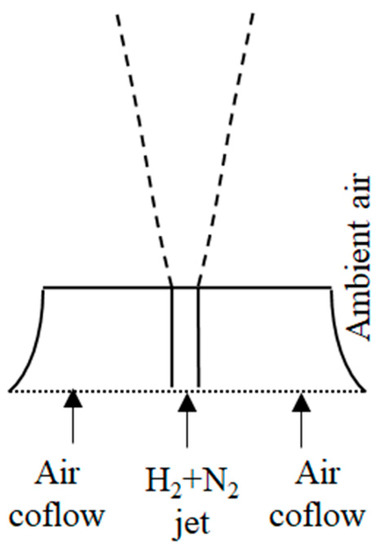
Figure 1.
Sketch of experimental set-up of Sautet and Stepowski [43].
The considered experimental conditions are listed in Table 1.

Table 1.
Experimental conditions for non-reacting H2/N2 jet [43] (V: Velocity; T: Temperature; d, D: Diameters of central and annular jets; Re: Reynolds number; Xi: Mole fractions).
2.2. Lifted H2/N2 Jet Flame
As the main test case, the atmospheric, lifted flame of a H2/N2 jet in vitiated co-flow was considered, which was investigated experimentally by Wu et al. [23]. A sketch of the configuration is presented in Figure 2.

Figure 2.
Sketch of experimental set-up of Wu et al. [19,23].
The fuel jet is positioned at the center of a disk with perforations, which supports a large number of lean premixed flames that provide a hot co-flowing stream. The central fuel jet protrudes about 70 mm over the perforated disk. Thus, it can be assumed that the central fuel jet issues into a homogeneous composition of the vitiated co-flow. The latter consists of the combustion products of an H2/Air mixture, which delivers the inlet boundary conditions for the calculation of the lifted flame. The test conditions for two typical cases for different co-flow conditions (Flame A and Flame B) with different H2/Air ratios are represented in Table 2.
Table 2.
Experimental conditions for lifted H2/N2 jet flame [23] (V: Velocity; T: Temperature; d, D: Diameters of central and annular jets; Re: Reynolds number; Qi: Volume flow rates).
In the present study, seven cases with seven different co-flow temperatures were considered (1010, 1013, 1020, 1030, 1040, 1044, and 1050 K). The different co-flow temperatures result from different H2/Air ratios of the co-flow. The corresponding compositions of the vitiated co-flow were calculated using the chemical kinetics code Cantera [44]. In doing so, the following procedure was applied: With the experimentally given flow rates of H2 and Air (Table 2), the complete combustion of the mixture was calculated assuming a well-stirred reactor. First, an adiabatic reactor was considered. In such calculations, the resulting exhaust gas temperatures turned out to be larger than the measured ones (Table 2). This is attributed to the heat loss in the experimental combustion device. Thus, in the well-stirred reactor calculations, a sufficient amount of heat loss was considered to obtain the experimental exhaust gas temperatures. The resulting exhaust gas composition was then taken as the composition to be used as the inlet boundary condition for the subsequent (main) calculation of the lifted jet flame. The considered co-flow temperatures and the corresponding gas compositions (calculated as mentioned above) are displayed in Table 3.
Table 3.
Considered co-flow temperatures and compositions for lifted H2/N2 jet flame [23] (T: Temperature; Xi: Mole fractions).
In the study of Cabra et al. [21], a single flame for a single co-flow temperature (1045 K) was published that was rather high to lead to a rather moderate lift-off height (H/d = 10). A different and interesting feature of the presently considered experiments of Wu et al. [23] is the investigation of a number of flames for a range of co-flow temperatures (1010–1050 K). The lift-off height increases with decreasing co-flow temperatures and the focus of the present study is the predictability of this relationship. For the present class of flames, autoignition and flame propagation, both, were reported to play a role [21,22,23,24]. For the flame of Ref. [21] with a moderate lift-off height, it was postulated that the transient startup was governed by autoignition, where the subsequent flame stabilization was affected by flame propagation in partial premixing. However, for varying co-flow temperatures, a shift in the relative importance of the mechanisms can be expected. Obviously, both processes, i.e., the autoignition and flame propagation (laminar flame speed), are strongly temperature-dependent, correlating with the observed [23] influence of the co-flow temperature (where the differential/preferential diffusion can also play role for the laminar flame speed of hydrogen flames). On the other hand, the temperature and composition of the burnable mixture that influence the chemical kinetics depend on the mixing that is strongly affected by the turbulent flow field.
3. Modeling
In this section, the modeling details are described in two sub-sections. In the first sub-section, an outline of the complete mathematical and numerical modeling is given. Combustion modeling is described separately in the subsequent sub-section.
3.1. Outline of the Mathematical and Numerical Modeling
An ideal gas mixture with Newtonian behavior was assumed. Possible buoyancy effects were omitted. This was justified by the prevailing high Froude numbers [45], indicated by the inlet conditions. Heat transfer due to radiation [46] was also omitted, assuming an adiabatic system. The molecular properties were modeled accurately. The specific heat capacity of each species was calculated via a pair of fourth order polynomials of temperature [47] (for low and high ranges of temperature). The molecular transport properties such as the viscosity, thermal conductivity, and the binary diffusion coefficients were obtained from the kinetic theory [14,48]. The multi-component diffusion in the mixture was treated by assuming Fickian diffusion, assuming “effective” binary diffusion coefficients [14]. This was considered to be a sufficiently accurate approach for mixtures having a species in excess [49], which was nitrogen in the present case. For some of the turbulent combustion models, an equality of the molecular Schmidt numbers was assumed, as will be indicated below.
As discussed above, turbulence was modeled within a RANS framework. Since the considered geometries and boundary conditions were axi-symmetric, the sought steady-state RANS solution also needed to be axi-symmetric. Thus, a two-dimensional axi-symmetric formulation was adapted.
As RANS turbulence models, two-equation turbulent viscosity models were considered [20]. Although higher order closures such as RSM [20] are potentially more accurate, they were not considered, since their application in the industrially relevant problems remained restricted due to the increased computational overhead and convergence problems encountered frequently. Among the turbulent viscosity-based turbulence models, those relying on the specific dissipation rate (omega, ω) are being increasingly used [50]. Nonetheless, since the present flow was of free-shear type, the turbulent viscosity models that are based on the dissipation rate (epsilon, ε) were considered only. The Standard k-ε [51], the RNG k-ε [52] (RNG: Renormalization group theory), and the Realizable k-ε models [53] were used. For modeling the turbulent fluxes of scalar quantities, the gradient–diffusion assumption was employed. In doing so, constant turbulent Prandtl-Schmidt numbers were assumed, assigning the value of 0.85 for the energy equation, and the value 0.7 for the remaining scalar transport equations. At the inlet boundaries, the boundary conditions of the turbulence variables were always determined by assuming a turbulence intensity of 4% (along with a locally isotropic turbulence) and a macro length scale based on the jet diameters [20].
The SIMPLEC pressure correction method [54] was used to treat the coupling of the velocity and pressure fields. For the discretization of the convective terms, the QUICK algorithm [55] was employed with a third order formal accuracy. The multi-purpose, finite volume method-based CFD code ANSYS Fluent 18.0 [56] was employed in the computational analysis. No special ad-hoc modifications tailored to the present type of problem were applied in the turbulence and turbulence combustion models. Thus, the standard settings [56] should be assumed for any model, unless the contrary is explicitly stated.
3.2. Combustion Modeling
3.2.1. Reaction Mechanisms
Two single-step global reaction mechanisms were considered (that include only the main species, H2, O2, H2O). These are the mechanism of Kudriakov et al. [57] (KU) and the mechanism of Marinov et al. [58] (MA). The former and latter assume an irreversible and a reversible reaction, respectively.
As the detailed reaction mechanisms, four mechanisms were considered. Each of them comprise about 20 elementary reactions (without counting the reverse ones) between the eight main and intermediate species, namely, H2, O2, H2O, H, O, OH, HO2, and H2O2. The considered detailed mechanisms are the Gri-Mech 2.11 [27] (G2), Gri-Mech 3.0 [59] (G3), the mechanisms of Conaire et al. [60] (CO), Keromnes et al. [61] (KE), and Li et al. [33] (LI). Gri-Mech 2.11 and Gri-Mech 3.0 are mechanisms that are optimized to model natural gas combustion, whereas the mechanism of Keromnes et al. is designed for syngas combustion. In using these mechanisms, the carbon- and nitrogen-containing species and reactions are stripped off. The mechanisms of Conaire et al. and Li et al. were developed specifically for hydrogen combustion.
A reversible reaction with N species can be represented as:
where and stay for the species and the related stoichiometric coefficients, while kf and kb represent rate coefficients of the forward and backward reactions, respectively.
According to the law of mass action, using the rate coefficients provided by the respective chemical reaction mechanism, the molar conversion rate of a species i according to chemical kinetics (RK,i) can be calculated as [14]:
where Ci stay for the species concentrations. The exponents ni are equivalent to for elementary reactions, as they may be different for empirical global reaction mechanisms. The rate coefficients are obtained by the Arrhenius equation [14], which is expressed for kf below.
where A, Ea, Ru, m denote the pre-exponential factor, activation energy, universal gas constant, temperature exponent, respectively, while T stays for the thermodynamic temperature.
Source terms of species transport equations are given by above expressions (Equation (2)). For a turbulent flow, within a RANS formulation, where time-averaged equations are solved, it is obvious that severe closure problems emerge due to the strong non-linearity of the source terms. Therefore, the so-called “turbulent combustion” models are needed that take the interaction between turbulence and chemistry, in an adequate manner into account. The presently considered turbulence combustion models are outlined below.
3.2.2. Turbulent Combustion Models
The presently considered turbulent combustion models are outlined in this subsection. Note that such models are, in general, quite complex, and details in their implementation may be influential on the results. The considered models refer to the versions as they are implemented in the used software ANSYS Fluent 18.0 [56].
Eddy Dissipation Model with Kinetics (EDM+K)
The time-averaged transport equations for each species are solved. The eddy dissipation model (EDM) assumes a mixing controlled combustion and calculates time-averaged conversion rates of the species based on the dissipation rate of turbulence eddies [62]. Here, the time-averaged molar conversion rate (REDM,i) is calculated from:
where , k, stay for the averaged mixture density, turbulence kinetic energy, and its dissipation rate, respectively. The terms Yi and Mi denote the averaged mass fraction of species i and its molar mass, respectively. The subscript R denotes each of the reacting species, whereas the subscript P refer to the sum of the product species. Coefficients , are empirical model constants. Standard values are used [62].
The chemical kinetics effects (K) are considered approximately, obtaining the conversion rates (RK,i) from the Arrhenius expressions of the underlying chemical reaction scheme by neglecting the fluctuations of the thermochemical variables, comparing the both rates and assigning the smaller one as the effective conversion rate [56]. Thus, the resulting time-averaged conversion rate is obtained from:
Due to the rather ad-hoc consideration of the chemical kinetics, the model makes sense only in combination with global reaction schemes. Therefore, this method is applied to Kudriakov et al. [57] (KU) and Marinov et al. [58] (MA) schemes, only. It is also to be noted that the MA scheme comprises a backward reaction, which is deactivated when applied in combination with this (EDM+K) turbulent combustion model.
Eddy Dissipation Concept (EDC)
The eddy dissipation concept (EDC) has evolved from the above-mentioned eddy dissipation idea [63] and exhibits slightly different versions that emerged in time. It can model the combined mixing and kinetics effects in a sounder manner compared to EDM+K. As the main modeling concept, it is assumed that reactions occur within small structures that are called fine-scales. The time-averaged source term (SEDC,i) of the species mass fraction transport equation is obtained from:
In Equation (5), the variables and represent the length fraction and time scale of the fine structures that relate to the volume and residence time of the assumed fine-scale reactors. These quantities are estimated from the velocity and length scales of turbulence. The variable denotes the fine-scale species mass fractions that are obtained after a reaction time of by solving chemical reactor equations. The version of the model that underlies the used software [56] corresponds to that of Gran and Magnussen [63]. Still, there are some deviations from the original model [63] in the implementation [56], such as the use of batch reactors to model the fine structures instead of perfectly stirred ones. In the present calculations, the direct integration method was applied in combination with the stiff chemistry solver [56] instead of making use of in situ adaptive tabulation (ISAT) [56]. The time-averaged transport equation was solved for each species, closing the source term as outlined above. Due to the rather sound modeling of turbulence-chemistry interaction, the model is generally observed to lead to good results in combination also with detailed reaction schemes.
Flamelet Generated Manifold (FGM)
According to the flamelet generated manifold (FGM) method [56,64], it is assumed that the realized trajectories on the thermochemical manifold of a turbulent flame can approximately be represented by the scalar evolution similar to that of a laminar flame. Under similar assumptions to the laminar flamelet method [65], the elemental mass fractions are associated with a single scalar quantity called mixture fraction (Z) that is governed by a source-free differential transport equation. The state of the reaction is described by an additional scalar variable, the so-called reaction progress variable (C) [64]. Thus, the thermochemical dependent variables can be expressed as unique functions of Z and C:
The functional relationships (Equation (6)) are obtained from one-dimensional laminar flame calculations that are performed in advance, and prepared in tabulated form for the subsequent CFD analysis. In the present application, the one-dimensional laminar flame calculations were performed based on a non-premixed (counterflow) configuration. About 100 different values of strain are considered, covering the whole spectrum from negligibly low strain up to extinction. Assuming that Z and C are statistically independent, the Favre-averaged values of the thermo-chemical variables () are obtained by integrating the relationships over the Z and C spaces, with the help of presumed probability density functions (Beta functions are used):
For the construction of the beta functions, modeled transport equations are solved for mean values (, ) and variances (, ) of Z, C [56,66,67]. The source term of the modeled equation is extracted from the one-dimensional laminar flame data like any other thermochemical variable. In constructing the beta functions, the mixture fraction and reaction progress variable space, each, are resolved by 41 points, while 21 points are used for the variances. The attractiveness of the method lies therein that it can incorporate detailed chemistry in a CFD calculation of turbulent combustion, with comparably quite low computational costs, since it requires the solution of only four differential transport equations (mean values and variances of Z and C), irrespective of the complexity of the underlying chemical reaction scheme. On the other hand, an assumption underlying the model is the equality of the molecular Schmidt numbers of the species transport equations (which is not necessary for EDM and EDC). Thus, the effects of differential and preferential diffusion [13,14] that are known to be important for flames of hydrogen containing fuels cannot be considered.
Composition PDF Transport (PDF)
To determine the averaged values of the thermochemical quantities, a single-point, joint probability density function (PDF) can be obtained from its transport equation. The joint probability density function represents the time fraction that the mixture spends at each species, temperature, and pressure state, leading to an (N + 2) dimensional joint probability density function for N species, temperature, and pressure spaces. The transport equation for the Favre composition probability density function (P) can be derived from the governing equations as:
In Equation (8), and denote the Favre mean and fluctuation values of the velocity vector. is the reaction rate for species k, while and denote the composition space and molecular diffusion flux vectors, respectively. The terms express the conditional probability of event A, given that event B occurs. The terms on the left-hand side are closed. The third term (which is closed) is the change due to chemical reactions, which makes up the strength of the method [25,56]. The right-hand side terms need to be modeled. The first term on the right-hand side, i.e., the turbulent flux term, is approximated by a gradient-diffusion approximation. The second right-hand side term is due to molecular mixing/diffusion. For its modeling, the Euclidian minimum spanning tree (EMST) model is applied [68], which is known to be more accurate than the alternatives models [56] such as the modified curl (MC) and interaction by exchange with the mean (IEM). Reaction source terms are obtained by direct integration, which was affordable in the present two-dimensional application. A Lagrangian Monte-Carlo method was adopted to solve the PDF transport equation. The number of particles per cell was chosen to be 50, which was shown by Cao et al. [42] to lead to a deviation of around 1% for the main species compared to the calculation with 100 particles per cell.
4. Results
4.1. On Solution Domains, Boundary Conditions, Grids
The two-dimensional axisymmetric solution domains of the non-reacting H2/N2 jet (Section 2.1) and the lifted H2/N2 flame (Section 2.2) have the same topology. The domains have a rectangular shape in the plane of axial (x) and radial (r) coordinates, which is depicted in Figure 3, with indications of the domain size and boundary types.
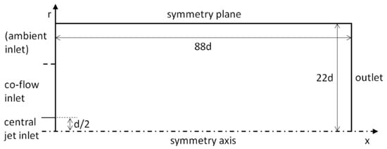
Figure 3.
Sketch of solution domain (not to scale).
At the outlet boundary, a constant static pressure is prescribed, along with zero-gradient conditions for the remaining variables. For the lifted flame (Section 2.2), the left boarder of the domain boundary is completely covered by the central jet and co-flow inlet boundaries. For the isothermal case (Section 2.1), the co-flow inlet extends up to a radial position of approximately 6d (indicated by a dashed line in the figure), where the remaining outer part (ambient inlet, Figure 3) is defined to be a pressure boundary that allows an inflow, i.e., suction of ambient air by the ejector effect.
At the central jet and co-flow inlet boundaries, uniform profiles are prescribed in accordance with the measured values (Table 1, Table 2 and Table 3). A minor influence of the profile shapes was reported by Cao et al. [42] in a similar study. Computational grids were generated as structured, rectangular grids with axial and radial clustering of the cells near the jet inlet.
4.2. Non-Reacting H2/N2 Jet
For obtaining a sufficiently accurate grid resolution, a grid independence study was conducted. In doing so, the Standard k-ε model was employed as the turbulence model. Figure 4 shows the predicted length (L) of the potential core (non-dimensionalized by d) as a function of grid resolution, where N represents the total number of grid nodes. It can be observed that a satisfactory grid independence was achieved for N ≥ 5000. In the subsequent computations for validating turbulence models, the grid with the highest resolution, i.e., the one with approximately 16,000 nodes, was used.
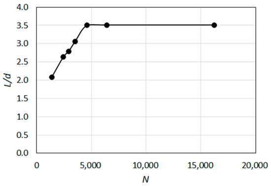
Figure 4.
Variation of predicted length of the potential core with grid resolution (isothermal test case).
The profiles of the calculated half value radius (δ) along the jet axis were compared with the measurements [43] in Figure 5. It can be observed that the results obtained by the Standard k-ε model show a quite well agreement with the measured values, which is better than those of the Realizable and RNG versions, for the current isothermal, variable density jet system. Thus, the Standard k-ε model was selected as the turbulence model for the subsequent study of the lifted H2/N2 flame.
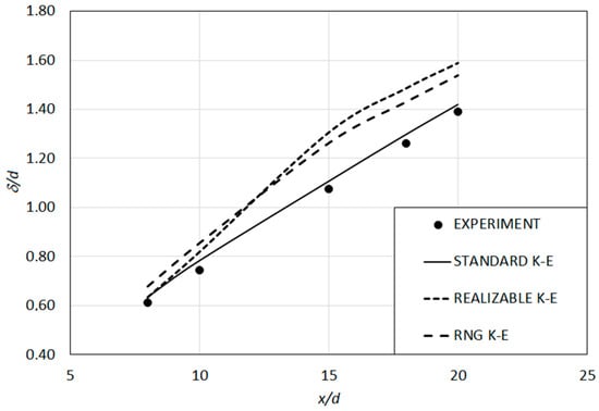
Figure 5.
Variation of predicted half value radius along jet axis (isothermal test case).
4.3. Lifted H2/N2 Jet Flame
A grid independence study was conducted also for the lifted H2/N2 jet flame. In Figure 6, the profile of the calculated centerline temperature (T) at ten jet diameters downstream the jet inlet (x/d = 10) for six different grids with varying number of total nodes (N) (obtained by the KU-EDM+K) approach) is presented. It can be observed that a satisfactory grid independence is obtained for the finer grids. In the further calculations, the finest grid, having approximately 16,000 nodes, was used. This complies well with the previous studies, where a grid independence was reported even for coarser grids with about 10,000 nodes.
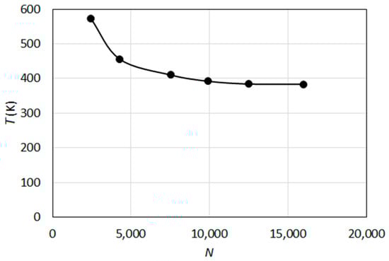
Figure 6.
Variation of calculated centerline temperature at x/d = 10 with grid resolution (KU-EDM+K).
Not all turbulent combustion models were used in combination with all reaction mechanisms. An overview of the investigated combinations is provided in Table 4, where a cross (X) means that the combination was investigated, and a minus (−) means that the combination was not considered.
Table 4.
Investigated combinations of turbulent combustion models and reaction mechanisms.
As mentioned before, the models were assessed based on their prediction accuracy of the lift-off height as a function of co-flow temperature. In many of the previous computational investigations (e.g., [42]) of similar cases, the flame root was marked in terms of the OH mass fraction. Since this cannot be applied while using a global/reduced reaction mechanism without comprising OH species, a temperature-based criterion was used in the present study, which is more general, in this sense. The flame root location, i.e., the lift-off height (H) was defined to be given by the position, where the local Favre-averaged temperature exceeds the co-flow temperature by 5 K (at any radius). This is exemplarily illustrated in Figure 7, where the predicted temperature fields by the G2-PDF approach are displayed for two co-flow temperatures, namely, for TCO = 1050 K (left) and TCO = 1010 K (right). In the figure, a sub-region in the nearfield of the central jet is displayed, with a size of 30d × 10d. According to the present approach, the flame root location is marked by the attainment of the local temperature values of 1055 K and 1015 K, for TCO = 1050 K and TCO = 1010 K, respectively. The corresponding isotherms T = 1055 K (left) and T = 1015 K (right) are also indicated in the figure. Thus, the lift-off height (H) is defined to be the distance between the inlet boundary and the nearest point of the corresponding isotherm to the inlet, as illustrated in Figure 7.
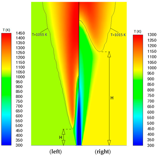
Figure 7.
Temperature field distributions and isotherms predicted by G2-PDF with indication of lift-off heights (left) for TCO = 1050 K, with isotherm T = 1055 K, (right) for TCO = 1010 K, with isotherm T = 1015 K.
No flame lift-off could be predicted by the global reaction mechanism of Kudriakov et al. In combination with both turbulent combustion models (KU-EDM+K, KU-EDC), the predicted flame remained attached to the burner rim for all values of the co-flow temperature within the range 1010–1050 K.
The results obtained by the global reaction mechanism of Marinov et al. in combination with different turbulent combustion models are shown in Figure 8, where the lift-off height (H) is presented as a function of the co-flow temperature. The measured values by Wu et al. are also shown in the figure.
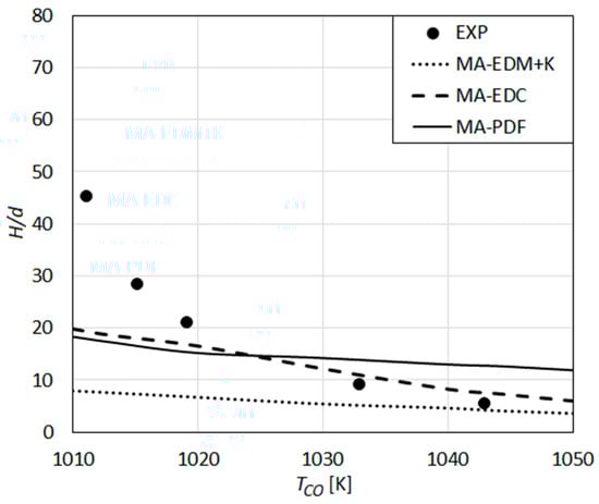
Figure 8.
Lift-off height as a function of co-flow temperature: Predictions using the global reaction mechanism of Marinov et al. [58] compared with the measurements of Wu et al. [23].
One can see that the strong dependence of the experimental lift-off height on the co-flow temperature is under-predicted (Figure 8). In combination with all three combustion models, a quite weak increase of H with decreasing TCO is predicted. The slope of the MA-EDC curve is closer to that of the experimental curve, compared to MA-EDM+K and MA-PDF curves, especially for the higher values of TCO, where a rather good quantitative agreement with the experiments and MA-EDC curve is observed.
The lift-off heights predicted by the detailed reaction mechanism GRI-Mech 3.0 in combination with different turbulent combustion models are compared with the measurements of Wu et al. in Figure 9.
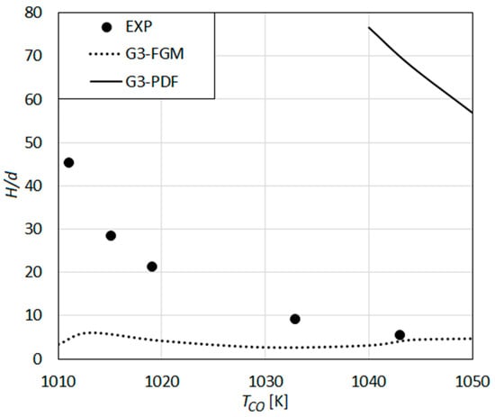
Figure 9.
Lift-off height as a function of co-flow temperature: Predictions using the detailed reaction mechanism GRI-Mech 3.0 [59] compared with the measurements of Wu et al. [23].
Using the eddy dissipation concept as the turbulent combustion model (G3-EDC), a stable lifted flame could not be obtained for the whole range of co-flow temperatures. A blow-off was always observed. Thus, a G3-EDC curve is missing in the figure. Applying the composition transport PDF method (G3-PDF), a lifted flame with a very large lift-off height of about H/d ≈ 55 is predicted for the highest co-flow temperature of 1050 K, which increases to H/d ≈ 75 for TCO = 1040 K. For lower values of TCO, the flame is blown-off (or, moves out of the solution domain). The predicted values (H/d > 55) for TCO > 1040 K are obviously very much higher than the measured values.
Applying the flamelet generated manifold method as the turbulent combustion model (G3-FGM), the predicted value agrees very well with the measured value (H/d ≈ 5) for high TCO (TCO > 1040 K) (Figure 9). However, the increase of the lift-off height with decreasing co-flow temperature is not predicted, as the lift-off height remains rather unaffected by TCO (even showing a slight reverse trend for some values of TCO). A similar behavior is observed also for the remaining detailed reaction mechanisms using the FGM as the turbulent combustion model, where the model cannot predict the dependence of H onto TCO. This may be seen to imply that the assumptions underlying FGM lose their validity for conditions prevailing for decreasing co-flow temperatures. The assumption of species Schmidt numbers to be equal (and Lewis number being unity), which is an essential part of FGM, but not required for the other turbulent combustion models, may also be a cause of the inaccuracy. Furthermore, the present approach of generating the one-dimensional laminar flame data based on a non-premixed configuration may be less adequate for large lift-off heights, with increasing degree of premixing. Moreover, the lack of ability of the presently applied procedure (FGM) for considering the autoignition effects can be seen as a further reason for the observed inferior performance.
The results obtained by the detailed reaction mechanism GRI-Mech 2.11 in combination with different turbulent combustion models are presented in Figure 10, where the experimental results of Wu et al. are also displayed.
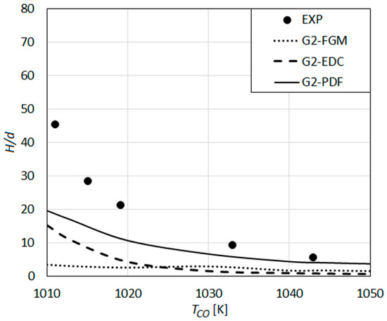
Figure 10.
Lift-off height as a function of co-flow temperature: Predictions using the detailed reaction mechanism GRI-Mech 2.11 [27] compared with the measurements of Wu et al. [23].
G2-EDC and G2-PDF show a qualitative agreement with the measurements, where they under-predict the measured values quantitatively. The under-prediction increases with decreasing co-flow temperatures, i.e., increasing lift-off heights. The G2-PDF results agree quite well with the measurements for high TCO (TCO > 1040), also showing a quantitatively better agreement with the experiments compared to the G2-EDC ones.
The observed difference in the predictions of the Gri-Mech 3.0 (G3) (Figure 9) and the Gri-Mech 2.11 (G2) (Figure 10) is quite substantial. This, and an even better performance of the earlier version of the mechanism (Gri Mech 2.11), were not necessarily expected. The modifications in the H2-related reactions in between the versions seem to imply a strong difference for H2 combustion. The observed relative performance of the schemes (Figure 9 vs. Figure 10) can be seen to be in line with the published comparisons [69], in which the premixed hydrogen-air flame speeds by Gri-Mech 2.11 were found to be larger than those of Gri-Mech 3.0. On the other hand, it should be noted that the observed performance of Gri-Mech 3.0 (which was optimized for natural gas) for hydrogen flames cannot fully be attributed to the mechanism itself, but should be seen in combination with the applied RANS framework, which is intrinsically less accurate in resolving flame structure/heat release patterns compared to higher order methods such as LES.
The predictions based on the detailed reaction mechanism of Conaire et al., in combination with various turbulent combustion models, are compared with the experimental results of Wu et al. in Figure 11.
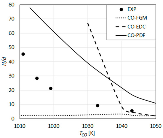
Figure 11.
Lift-off height as a function of co-flow temperature: Predictions using the detailed reaction mechanism of Conaire et al. [60] compared with the measurements of Wu et al. [23].
The results obtained by the composition PDF transport model (CO-PDF) as the turbulent combustion model show a qualitative agreement with the measured values. Nonetheless, quantitatively, the experimental values are highly over-predicted (Figure 11).
The results obtained by the eddy dissipation concept (CO-EDC) (Figure 11) show a qualitatively different behavior compared to that observed for Gri-Mech 2.11 (Figure 10). The G2-EDC curve shows a continuous increase of H with decreasing TCO (Figure 10). CO-EDC exhibits two regions with different qualitative behaviors (Figure 11). For high TCO (TCO > 1040 K), i.e., low values of H, CO-EDC shows a slowly increasing H with decreasing TCO, and a good quantitative agreement with the measurements. However, for lower TCO values (TCO < 1400), a very rapid, abrupt increase of H is observed with decreasing TCO (with a remarkable over-prediction of the measured values), which quickly leads to blow-off beyond TCO < 1030 K (Figure 11).
The lift-off heights that are predicted by the reaction mechanism of Keromnes et al. using different turbulent combustion models are compared with the experimental results of Wu et al. in Figure 12.
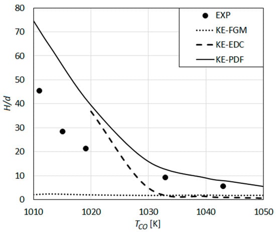
Figure 12.
Lift-off height as a function of co-flow temperature: Predictions using the detailed reaction mechanism of Keromnes et al. [61] compared with the measurements of Wu et al. [23].
Qualitatively, the predictions obtained by the Keromnes et al. mechanism (Figure 12) show a similar behavior to that observed for the Conaire et al. mechanism (Figure 11). Quantitatively, the predicted values by EDC (KE-EDC) and PDF (KE-PDF) turbulent combustion models agree better with the experiments (Figure 12) than the CO-EDC and CO-PDF do (Figure 11). The KE-PDF curve predicts lower H values compared to the CO-PDF curve and is much closer to the experimental curve (Figure 12). For TCO > 1030 K, the predicted values by KE-PDF agree rather well with the experimental ones. For TCO < 1030 K, a remarkable over-prediction by KE-PDF is still observed. The results by EDC model (KE-EDC) (Figure 12) are qualitatively similar to those of CO-EDC (Figure 11), showing first a shallow increase with decreasing TCO, followed by a rapid increase and blow-off by a further decrease of TCO. Compared to CO-EDC (Figure 11), the characteristic TCO values are lower for KE-EDC (Figure 12). The border between the two regimes is about TCO ≈ 1030 K and the blow-off occurs for TCO < 1020 K (the values were 1040 K and 1030 K for CO-EDC).
The results obtained by the detailed reaction mechanism of Li et al. in combination with different turbulent combustion models are displayed in Figure 13, where the lift-off height (H) is presented as a function of the co-flow temperature. The measured values by Wu et al. are also displayed in the figure.
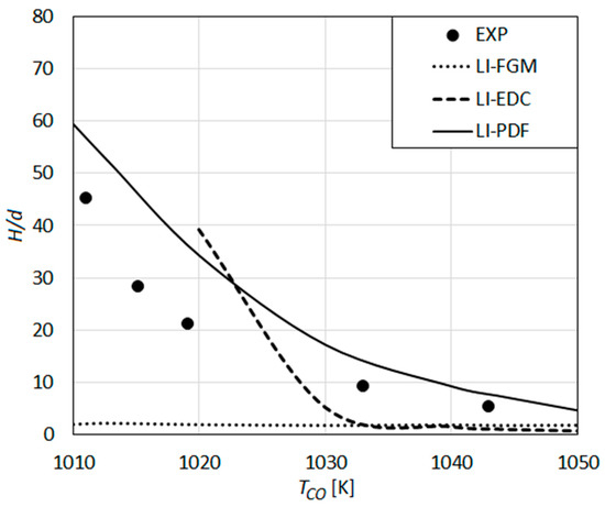
Figure 13.
Lift-off height as a function of co-flow temperature: Predictions using the detailed reaction mechanism of Li et al. [33] compared with the measurements of Wu et al. [23].
The predictions obtained by the mechanism of Li et al. (Figure 13) using different turbulent combustion models are qualitatively similar to those obtained by the Keromnes et al. mechanism (Figure 12). LI-FGM and LI-EDC curves (Figure 13) are also quantitatively very close to KE-FGM and KE-EDC (Figure 12), respectively. The results obtained by the composition PDF transport model (LI-PDF) are (Figure 13), quantitatively, closer to the experimental curve compared to the results by KE-PDF (Figure 12). Among all of modeling approaches considered, the Li et al. mechanism [33] combined with the composition PDF transport model [25] provides the best overall agreement with the experiments for the lift-off height (Figure 13). However, the prediction accuracy by LI-PDF still leaves much to be desired, as measured lift-off height is remarkably over-predicted, especially for rather low TCO values.
As an attempt for a better understanding of the mechanisms and performance of the modeling approaches, the important parameters of chemical kinetics were also analyzed. For different mixtures of the central jet and co-flow streams at different equivalence ratios (ϕ), the ignition delay time τIGN, and the laminar flame speed SL (undisturbed, planar flame) were calculated using the above-mentioned detailed reaction mechanisms, using the chemical kinetics code Cantera [44]. Note that the calculations hold for premixed conditions for each equivalence ratio, and, thus, the results (Figure 14) can only be used as indications for the present partially premixed situation.
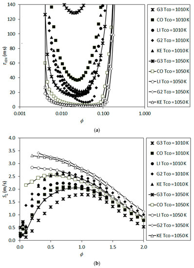
Figure 14.
Chemical kinetics parameters predicted by different detailed reaction mechanisms as function of equivalence ratio for the mixtures of the central jet and co-flow stream with varying temperature, (a) ignition delay time and (b) laminar flame speed (undisturbed planar flame).
Figure 14 illustrates the calculated ignition times (Figure 14a) and laminar flame speeds (Figure 14b) as a function of the equivalence ratio, for two different temperatures of the co-flow stream, i.e., for TCO = 1010 K and TCO = 1050 K, spanning the whole considered range. Note that for a given co-flow temperature, the temperature of the mixture changes remarkably with changing equivalence ratio, due to the large difference between the jet and co-flow temperatures.
One can see that the ignition delay times are quite long for ~0.2 < ϕ and ϕ < ~0.005, due to the too low mixture temperatures for the former, and too low fuel mass fractions for the latter (Figure 14a). Within the region ~0.005 < ϕ < ~0.2, finite ignition delay times are predicted in all cases, mainly due to the high mixture temperature although the mixture is very fuel-lean. A rough estimation of the convective residence time can be done based on the co-flow inlet velocity and domain length, which gives a value of about 100 ms. This is within the range of the ignition delay times that occur in Figure 14a, and indicates the likeliness of autoignition for the present problem.
The laminar flame speeds are also quite high for the fuel-lean values of the equivalence ratio, due to the high mixture temperatures (Figure 14b). For some cases, values for very fuel-lean mixtures are not plotted due to the occurrence of autoignition events, hindering the determination of flame speed in classical sense. Note that the calculated laminar flame speed values (Figure 14b) cope well with the flow velocity, which may roughly be characterized by the co-flow inlet velocity of 4 m/s.
The calculated ignition delay times and laminar flame speeds (Figure 14) agree qualitatively well with the predicted performance of the detailed reaction mechanisms shown in the previous figures (Figure 9, Figure 10, Figure 11, Figure 12 and Figure 13). The high values of the lift-off height correlate with the high values of the ignition delay time and low values of the laminar flame speed, as one would expect.
An inspection of the ignition delay times for all considered detailed reaction mechanisms show that the shortest ignition delay times occur for equivalence ratios (ϕ) within the range 0.02–0.05. Variation of the radial coordinate as a function of the axial coordinate along these isolines of the equivalence ratio (ϕ = 0.02, ϕ = 0.05) are plotted in Figure 15. These isolines are obtained from a non-combusting calculation (pure mixing) for TCO = 1010 K. Additionally, the coordinates of the flame roots (the flame anchoring positions used in determining the lift-off heights, H, as illustrated in Figure 7) are plotted in the figure, as predicted by different detailed reaction mechanisms using the PDF (Figure 15a) and EDC (Figure 15b) turbulent combustion models.
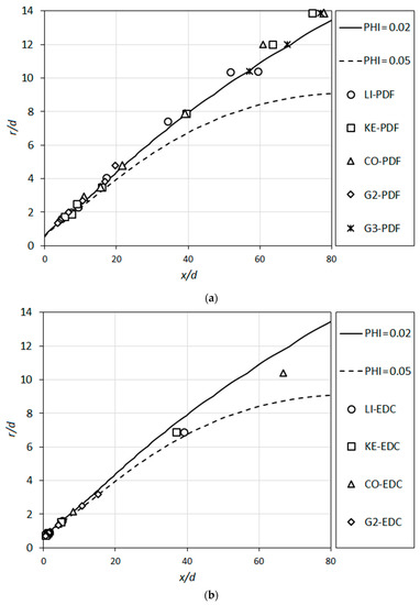
Figure 15.
Isolines of ϕ = 0.02 and ϕ = 0.05 predicted for non-combusting flow compared with the predicted flame root positions based on different detailed reaction mechanisms, using the (a) PDF turbulent combustion model and the (b) EDC turbulent combustion model.
It is interesting to observe that the predicted flame root positions lie very close to the region of shortest autoignition times (Figure 14a) for all cases (Figure 15). This implies that autoignition is very likely to play the major role in anchoring the flame. On the other hand, the very rapid increase of the autoignition time with the variation of the equivalence ratio indicates that the flame propagation phenomenon is likely to be dominant in the other regions of the flame front, determining its shape.
It is also interesting to note that the predictions obtained by PDF lie quite close to the ϕ = 0.02 curve (Figure 15a), whereas the EDC results turn out to be closer to the ϕ = 0.05 curve (Figure 15b).
For a fuller assessment of the overall performance of the different modeling approaches, the Central Processing Unit (CPU) times were compared. The mechanisms of Marinov et al. [58] and Li et al. [33] were taken as the representative global and detailed reaction mechanisms, respectively. The CPU times required for the same number of iterations are compared in Figure 16. The CPU times are scaled in such a way that the largest CPU time (which is for the detailed reaction mechanism in combination with the PDF) takes the value of 1000.
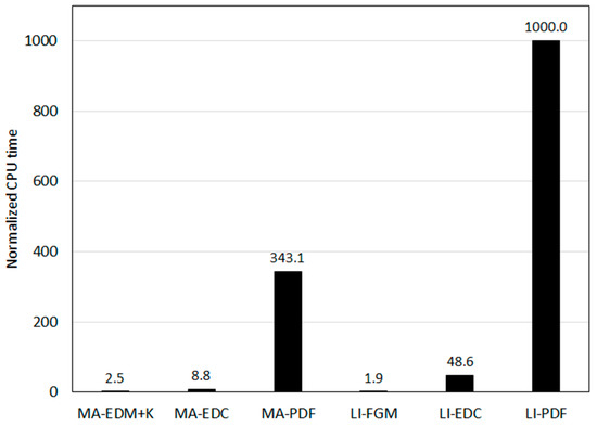
Figure 16.
Comparison of the CPU times for the same number of iterations.
Obviously, the PDF turbulent combustion model leads to very much larger CPU times in comparison to the alternative modeling approaches, even in combination with a global reaction mechanism, which is the main obstacle for the use of this potentially most accurate model in complex, three-dimensional problems. The lowest CPU time is demanded by the FGM turbulent combustion model, although it integrates a detailed reaction mechanism. Unfortunately, the model turns out to be quite inaccurate for the present problem.
5. Conclusions
Lifted H2/N2 flame in vitiated co-flow was computationally investigated within a RANS approach for turbulence modeling. Global and detailed reaction mechanisms were applied in combination with different models for turbulent combustion. The focus of the investigation was the prediction of the lift-off height that varies with varying co-flow temperature. Predictions were compared with published measurements of other authors.
The results indicate that an accurate numerical prediction of the lifted hydrogen flame is, generally, a very challenging task, especially for low co-flow temperatures, i.e., for large lift-off heights. For rather low experimental lift-off heights (H/d < 10), some modeling approaches deliver fairly accurate results. For higher values of the experimental lift-off height, all modeling approaches show a rather large deviation from the experimental value.
Among the considered global reaction mechanisms, the mechanism of Marinov et al. [58] is observed to be able to predict the lift-off phenomenon when applied in combination with the eddy dissipation model (EDM+K) [56,62], eddy dissipation concept (EDC) [56,63], and composition PDF transport (PDF) [25,56] as the turbulent combustion model. However, the sensitivity of the lift-off height to the co-flow temperature is under-predicted. For low H/d (H/d < 10), EDM+K, and EDC, the results show a fair agreement with the experiments.
It is observed that Gri-Mech 3.0 [59] and Gri-Mech 2.11 [27] perform very differently. Gri-Mech 3.0 predicts complete blow-off or extremely large lift-off (at high co-flow temperatures in combination with PDF), whereas Gri-Mech 2.11 generally under-predicts the lift-off height, while delivering a quite good agreement with the measurements for H/d < 10, combined with the PDF turbulent combustion model.
The flamelet generated manifold (FGM) [56,63] turbulent combustion modeling approach, when used with a detailed reaction mechanism, predicts a rather small lift-off that may show a fair agreement with the experimental value only for high co-flow temperatures for some reaction mechanisms. However, the sensitivity of the lift-off height to the co-flow temperature is not predicted, leading to a strong under-prediction for all higher values of the co-flow temperature.
The results obtained by the detailed reaction mechanisms of Conaire et al. [60], Keromnes et al. [61], and Li et al. [33] show a similar qualitative behavior. The results obtained by the EDC turbulent combustion model exhibit two different characteristics for high and low co-flow temperature ranges. The predicted lift-off height varies rather weakly in the high co-flow temperature range. In the low co-flow temperature range, a quite steep increase of the lift-off height is observed, leading to a rapid blow-off. The predictions delivered by PDF as the turbulent combustion model agree qualitatively well with the measurements. As the results obtained by the Conaire et al. mechanism strongly over-predict the experimental values, the predictions of the Li et al. mechanism show the closest agreement with the experiments. Although the Li et al. mechanism combined with the PDF turbulent combustion model delivers the best agreement with the measurements, its accuracy still leaves much to be desired for low co-flow temperatures, where the increasing lift-off heights are remarkably over-predicted.
Author Contributions
Conceptualization, A.C.B.; methodology, A.C.B.; validation, A.C.B. and B.P.; formal analysis, A.C.B. and B.P.; investigation, A.C.B. and B.P.; resources, B.P.; data curation, B.P.; writing—original draft preparation, A.C.B.; writing—review and editing, A.C.B. and B.P.; visualization, A.C.B. and B.P.; supervision, A.C.B.; project administration, A.C.B. All authors have read and agreed to the published version of the manuscript.
Funding
This research received no external funding.
Conflicts of Interest
The authors declare no conflicts of interest.
References
- Benim, A.C.; Geiger, M.; Doehler, S.; Schoenenberger, M.; Roemer, H. Modelling the flow in the exhaust hood of steam turbines under consideration of turbine-exhaust hood interaction. In Proceedings of the 1st European Conference on Turbomachinery—Fluid Dynamic and Thermodynamic Aspects: Computational Methods, Erlangen, Germany, 1–3 March 1995; Book Series: VDI Berichte. VDI Verlag: Duesseldorf, Germany, 1995; Volume 1185, pp. 343–357. [Google Scholar]
- Strielkowski, W.; Volkova, E.; Pushkareva, L.; Streimikiene, D. Innovative policies for energy efficiency and the use of renewables in hausholds. Energies 2019, 12, 1392. [Google Scholar] [CrossRef]
- Ebling, D.G.; Krumm, A.; Pfeiffelmann, B.; Gottschald, J.; Bruchmann, J.; Benim, A.C.; Adam, M.; Labs, R.; Herbertz, R.R.; Stunz, A. Development of a system for thermoelectric heat recovery from stationary industrial processes. J. Electron. Mater. 2016, 45, 3433–3439. [Google Scholar] [CrossRef]
- Tucki, K.; Orynycz, O.; Wasiak, A.; Świć, A.; Wichłacz, J. The impact of fuel type on the output parameters of a new biofuel burner. Energies 2019, 12, 1383. [Google Scholar] [CrossRef]
- Iqbal, S.; Benim, A.C.; Fischer, S.; Joos, F.; Kluß, D.; Wiedermann, A. Experimental and numerical analysis of natural bio and syngas swirl flames in a model gas turbine combustor. J. Therm. Sci. 2016, 25, 460–469. [Google Scholar] [CrossRef]
- Lamas, M.I.; Rodriguez, C.G. NOx reduction in Diesel-hydrogen engines using different strategies of ammonia injection. Energies 2019, 12, 1255. [Google Scholar] [CrossRef]
- Atakan, B. Compression-expansion processes for chemical energy storage: Thermodynamic optimization for methane, ethane and hydrogen. Energies 2019, 12, 3332. [Google Scholar] [CrossRef]
- Benim, A.C.; Epple, B.; Krohmer, B. Modelling of pulverised coal combustion by a Eulerian-Eulerian two-phase flow formulation. Prog. Comput. Fluid Dyn. Int. J. 2005, 5, 345–361. [Google Scholar] [CrossRef]
- Kim, J.-P.; Schnell, U.; Scheffknecht, G.; Benim, A.C. Numerical modelling of MILD combustion for coal. Prog. Comput. Fluid Dyn. Int. J. 2007, 7, 337–346. [Google Scholar] [CrossRef]
- Cordiner, S.; Manni, A.; Mulone, V.; Rocco, V. Biomass pyrolysis modeling of systems at laboratory scale with experimental validation. Int. J. Numer. Methods Heat Fluid Flow 2018, 28, 413–438. [Google Scholar] [CrossRef]
- Krakhella, K.W.; Bock, R.; Burheim, O.S.; Seland, F. Heat to H2: Using waste heat for hydrogen production through reverse electrodialysis. Energies 2019, 12, 3428. [Google Scholar] [CrossRef]
- El-Emam, R.S.; Khamis, I. Advances in nuclear hydrogen production: Results from an IAEA international collaborative research project. Int. J. Hydrogen Energy 2018, 44, 19080–19088. [Google Scholar] [CrossRef]
- Benim, A.C.; Syed, K.J. Flashback Mechanisms in Lean Premixed Gas Turbine Combustion; Academic Press: Cambridge, UK, 2014. [Google Scholar]
- Turns, S.R. An Introduction to Combustion, 3rd ed.; McGrawHill: New York, NY, USA, 2012. [Google Scholar]
- Lawn, C.J. Lifted flames on fuel jets in co-flowing air. Prog. Energy Combust. Sci. 2009, 35, 1–30. [Google Scholar] [CrossRef]
- Libby, P.A.; Williams, F.A. Turbulent Reacting Flows; Academic Press: London, UK, 1994. [Google Scholar]
- Schefer, R.W.; Namazian, M.; Kelly, J. Stabilization of lifted turbulent-jet flames. Combust. Flame 1994, 99, 75–86. [Google Scholar] [CrossRef]
- Benim, A.C.; Escudier, M.P.; Nahavandi, A.; Nickson, A.K.; Syed, K.J.; Joos, F. Experimental and numerical investigation of isothermal flow in an idealized swirl combustor. Int. J. Numer. Methods Heat Fluid Flow 2010, 20, 348–370. [Google Scholar] [CrossRef]
- Benim, A.C.; Pfeiffelmann, B.; Oclon, P.; Taler, J. Computational investigation of a lifted hydrogen flame with LES and FGM. Energy 2019, 173, 1172–1181. [Google Scholar] [CrossRef]
- Durbin, P.A.; Reif, B.A.P. Statistical Theory and Modelling for Turbulent Flows, 2nd ed.; Wiley: Chichester, UK, 2011. [Google Scholar]
- Cabra, R.T.; Myhrvold, T.; Chen, J.Y.; Dibble, R.W.; Karpetis, A.N.; Barlow, R.S. Simultaneous laser Raman-Rayleigh-LIF measurements and numerical modelling results of a lifted turbulent H2/N2 jet flame in a vitiated coflow. Proc. Combust. Inst. 2002, 29, 1881–1888. [Google Scholar] [CrossRef]
- Markides, C.N.; Mastorakos, E. An experimental study of hydrogen autoignition in a turbulent co-flow of heated air. Proc. Combust. Inst. 2005, 30, 883–891. [Google Scholar] [CrossRef]
- Wu, Z.; Stårner, S.H.; Bilger, R.W. Lift-off heights of turbulent H2/N2 jet flames in a vitiated co-flow. In Proceedings of the 2003 Australian Symposium on Combustion & The 8th Australian Flame Days, Melbourne, Australia, 8–9 December 2003; Honnery, D., Ed.; Monash University: Melbourne, Australia, 2003. [Google Scholar]
- Gordon, R.L.; Stårner, S.H.; Masri, A.R.; Bilger, R. Further characterization of lifted hydrogen and methane flames issuing into a vitiated coflow. In Proceedings of the Fifth Asia-Pacific Conference in Combustion, Adelaide, Australia, 18–20 July 2005. [Google Scholar]
- Pope, S.B. Computations of turbulent combustion: Progress and challenges. Proc. Combust. Inst. 1991, 23, 591–612. [Google Scholar] [CrossRef]
- Magnussen, B.F. The Eddy Dissipation Concept—A bridge between science and technology. In Proceedings of the ECCOMAS Thematic Conference on Computational Combustion, Lisbon, Portugal, 21–24 June 2005. [Google Scholar]
- Bowman, C.T.; Hanson, R.K.; Davidson, D.F.; Gardiner, W.C., Jr.; Lissianski, V.; Smith, G.P.; Golden, D.M.; Goldenberg, M.; Frenklach, M. Gri-Mech 2.11; Gas Research Institute: Des Plaines, IL, USA, 1999; Available online: www.me.berkeley.edu/gri-mech (accessed on 5 November 2018).
- Masri, A.R.; Cao, R.; Pope, S.B.; Goldin, G.M. PDF calculations of turbulent lifted flames of H2/N2 fuel issuing into a vitiated co-flow. Combust. Theory Model. 2004, 8, 1–22. [Google Scholar] [CrossRef]
- Wu, Z.; Masri, A.R.; Bilger, R.W. An experimental investigation of the turbulence structure of a lifted H2/N2 jet flame in a vitiated co-flow. Flow Turbul. Combust. 2006, 76, 61–81. [Google Scholar] [CrossRef]
- Mueller, M.A.; Kim, T.J.; Yetter, R.A.; Dryer, F.L. Flow reactor studies and kinetic modeling of the H2/O2 reaction. Int. J. Chem. Kinet. 1999, 31, 113–125. [Google Scholar] [CrossRef]
- Lee, J.; Kim, Y. DQMOM based PDF transport modeling for turbulent lifted nitrogen-diluted hydrogen jet flame with autoignition. Int. J. Hydrogen Energy 2012, 37, 18498–18508. [Google Scholar] [CrossRef]
- Mir Najafizadeh, S.M.; Sadeghi, M.T.; Soduteh-Gherebagh, R. Analysis of autoignition of a turbulent lifted H2/N2 jet flame issuing into a vitiated coflow. Int. J. Hydrogen Energy 2013, 38, 2510–2522. [Google Scholar] [CrossRef]
- Li, J.; Zhao, Z.; Kazakov, A.; Dryer, F.L. An updated comprehensive kinetic model of hydrogen combustion. Int. J. Chem. Kinet. 2004, 36, 566–575. [Google Scholar] [CrossRef]
- Mouangue, R.; Obounou, M.; Mura, A. Turbulent lifted flames of H2/N2 fuel issuing into a vitiated coflow investigated using Lagrangian Intermittent Modelling. Int. J. Hydrogen Energy 2014, 39, 13002–13013. [Google Scholar] [CrossRef]
- Borghi, R.; Gonzalez, M. Applications of Lagrangian models to turbulent combustion. Combust. Flame 1986, 63, 239–250. [Google Scholar] [CrossRef]
- Naud, B.; Novella, R.; Pastor, J.M.; Winklinger, J.F. RANS modelling of a lifted H2/N2 flame using an unsteady flamelet progress variable approach with presumed PDF. Combust. Flame 2015, 162, 893–906. [Google Scholar] [CrossRef]
- Ihme, M.; See, Y.C. Prediction of autoignition in a lifted methane/air flame using an unsteady flamelet/progress variable model. Combust. Flame 2010, 157, 1850–1862. [Google Scholar] [CrossRef]
- Saxena, P.; Williams, F.A. Testing a small detailed chemical-kinetic mechanism for the combustion of hydrogen and carbon monoxide. Combust. Flame 2006, 145, 316–323. [Google Scholar] [CrossRef]
- Klimenko, A.Y.; Bilger, R.W. Conditional moment closure for turbulent combustion. Prog. Energy Combust. Sci. 1999, 25, 595–687. [Google Scholar] [CrossRef]
- De, S.; De, A.; Jaiswal, A.; Dash, A. Stabilization of lifted hydrogen jet diffusion flame in a vitiated co-flow: Effects of jet and coflow velocities, coflow temperature and mixing. Int. J. Hydrogen Energy 2016, 41, 15026–15042. [Google Scholar] [CrossRef]
- Larbi, A.A.; Bounif, A.; Senouci, M.; Gökalp, I.; Bouzit, M. RANS modelling of a lifted hydrogen flame using Eulerian/Lagrangian approaches with transported PDF method. Energy 2018, 164, 1242–1256. [Google Scholar] [CrossRef]
- Cao, R.P.; Pope, S.B.; Masri, A.R. Turbulent lifted flames in a vitiated coflow investigated using joint PDF calculations. Combust. Flame 2005, 142, 438–453. [Google Scholar] [CrossRef]
- Sautet, J.C.; Stepowski, D. Dynamic behavior of variable density, turbulent jets in their near development field. Phys. Fluids 1995, 7, 2796–2806. [Google Scholar] [CrossRef]
- Goodwin, D.G.; Speth, R.L.; Moffat, H.K.; Weber, B.W. Cantera: An Object-Oriented Software Toolkit for Chemical Kinetics, Thermodynamics and Transport Processes; Version 2.4.0; 2018; Available online: https://www.cantera.org (accessed on 11 November 2018).
- So, R.M.C.; Aksoy, H. On vertical turbulent buoyant jets. Int. J. Heat Mass Transf. 1993, 36, 3187–3200. [Google Scholar] [CrossRef]
- Benim, A.C. A finite element solution of radiative heat transfer in participating media utilizing the moment method. Comput. Methods Appl. Mech. Eng. 1988, 67, 1–14. [Google Scholar] [CrossRef]
- Kee, R.J.; Rupley, F.M.; Miller, J.A. The Chemkin Thermodynamic Data Base; Sandia National Laboratories Report, SAND87-8215B; Sandia National Laboratories: Livermore, CA, USA, 1991. [Google Scholar]
- Hirschfelder, J.O.; Curtiss, C.F.; Bird, R.B. Molecular Theory of Gases and Liquids; John Wiley & Sons: New York, NY, USA, 1954. [Google Scholar]
- Kee, R.J.; Dixon-Lewis, G.; Warnatz, J.; Coltrin, M.E.; Miller, J.A. A Fortran Computer Code Package for the Evaluation of Gas Phase Multicomponent Transport Properties; Sandia National Laboratories Report SAND86-8246; Sandia National Laboratories: Livermore, CA, USA, 1990. [Google Scholar]
- Menter, F.R. Two-equation eddy-viscosity turbulence models for engineering applications. AIAA J. 1994, 32, 1598–1605. [Google Scholar] [CrossRef]
- Launder, B.E.; Spalding, D.B. The numerical computation of turbulent flows. Comput. Methods Appl. Mech. Eng. 1974, 3, 269–289. [Google Scholar] [CrossRef]
- Yakhot, V.; Orszag, S.A.; Thangam, S.; Gatski, T.B.; Speizale, C.G. Development of turbulence models for shear flows by a double expansion technique. Phys. Fluids 1992, 4, 1510–1520. [Google Scholar] [CrossRef]
- Shih, T.-H.; Liou, W.W.; Shabbir, A.; Yang, Z.; Zhu, J. A new k-ε eddy-viscosity model for high Reynolds number turbulent flows—Model development and validation. Comput. Fluids 1995, 24, 227–238. [Google Scholar] [CrossRef]
- Van Doormal, J.P.; Raithby, G.D. Enhancements of the SIMPLE method for predicting incompressible fluid flows. Numer. Heat Transf. 1984, 7, 147–163. [Google Scholar] [CrossRef]
- Leonard, B.P. A stable and accurate convective modelling procedure based on quadratic upstream interpolation. Comput. Methods Appl. Mech. Eng. 1979, 19, 59–98. [Google Scholar] [CrossRef]
- Engineering Simulation & 3D Design Software, ANSYS Fluent 18.0, Theory Guide. 2018. Available online: https://www.ansys.com (accessed on 28 November 2018).
- Kudriakov, S.; Studer, S.; Bin, C. Numerical simulation of the laminar hydrogen flame in the presence of a quenching mesh. Int. J. Hydrogen Energy 2011, 36, 2555–2559. [Google Scholar] [CrossRef]
- Marinov, N.M.; Westbrook, C.K.; Pitz, W.J. Detailed and Global Chemical Kinetics Model for Hydrogen; Lawrence Livermore National Laboratory Report UCRL-JC-120677; Lawrence Livermore National Laboratory: Livermore, CA, USA, 1995. [Google Scholar]
- Smith, G.P.; Golden, D.M.; Frenklach, M.; Moriarty, N.W.; Eiteneer, B.; Goldenberg, M.; Bowman, T.; Hansin, R.K.; Sing, S.; Gardiner, W.C., Jr.; et al. GRI-Mech. 2018. Available online: http://combustion.berkeley.edu/gri-mech/ (accessed on 11 November 2018).
- Conaire, M.O.; Curran, H.J.; Simmie, J.M.; Pitz, W.J.; Westbrook, C.K. A comprehensive modeling study of hydrogen oxidation. Int. J. Chem. Kinet. 2004, 36, 603–622. [Google Scholar] [CrossRef]
- Keromnes, A.; Metcalfe, W.K.; Heufer, K.A.; Donohoe, N.; Das, A.K.; Sung, C.J.; Herzler, J.; Naumann, C.; Griebel, P.; Mathieu, O.; et al. An experimental and detailed chemical kinetic modeling study of hydrogen and syngas mixture oxidation at elevated pressures. Combust. Flame 2013, 160, 995–1011. [Google Scholar] [CrossRef]
- Magnussen, B.F.; Hjertager, B.H. On mathematical models of turbulent combustion with special emphasis on soot formation and combustion. In Symposium (International) on Combustion; The Combustion Institute: Pittsburgh, PA, USA, 1976; pp. 719–729. [Google Scholar]
- Gran, I.R.; Magnussen, B.F. A numerical study of a bluff-body stabilized diffusion flame. Part 2. Influence of combustion modeling and finite-rate chemistry. Combust. Sci. Technol. 1996, 119, 191–217. [Google Scholar] [CrossRef]
- Van Oijen, A.; De Goey, L.P.H. Modelling of premixed laminar flames using flamelet-generated manifolds. Combust. Sci. Technol. 2000, 161, 113–137. [Google Scholar] [CrossRef]
- Peters, N. Turbulent Combustion; Cambridge University Press: Cambridge, UK, 2002. [Google Scholar]
- Poinsot, T.; Veynante, D. Theoretical and Numerical Combustion, 2nd ed.; Edwards: Philadelphia, PA, USA, 2005. [Google Scholar]
- Benim, A.C.; Iqbal, S.; Meier, W.; Joos, F.; Wiedermann, A. Numerical investigation of turbulent swirling flames with validation in a gas turbine model combustor. Appl. Therm. Eng. 2017, 110, 202–212. [Google Scholar] [CrossRef]
- Subramaniam, S.; Pope, S.B. A mixing model for turbulent reactive flows based on Euclidian minimum spanning trees. Combust. Flame 1998, 115, 487–514. [Google Scholar] [CrossRef]
- Fuel-Air Equivalence Ratio-Flame Speed Curve. Available online: http://combustion.berkeley.edu/gri_mech/version30/figs30/h2fl.gif (accessed on 18 November 2019).


© 2019 by the authors. Licensee MDPI, Basel, Switzerland. This article is an open access article distributed under the terms and conditions of the Creative Commons Attribution (CC BY) license (http://creativecommons.org/licenses/by/4.0/).