Abstract
In this paper, we present an assessment of methods for estimating and comparing the thermodynamic performance of working fluids for organic Rankine cycle power systems. The analysis focused on how the estimated net power outputs of zeotropic mixtures compared to pure fluids are affected by the method used for specifying the performance of the heat exchangers. Four different methods were included in the assessment, which assumed that the organic Rankine cycle systems were characterized by the same values of: (1) the minimum pinch point temperature difference of the heat exchangers; (2) the mean temperature difference of the heat exchangers; (3) the heat exchanger thermal capacity (); or (4) the heat exchanger surface area for all the considered working fluids. The second and third methods took into account the temperature difference throughout the heat transfer process, and provided the insight that the advantages of mixtures are more pronounced when large heat exchangers are economically feasible to use. The first method was incapable of this, and deemed to result in optimistic estimations of the benefits of using zeotropic mixtures, while the second and third method were deemed to result in conservative estimations. The fourth method provided the additional benefit of accounting for the degradation of heat transfer performance of zeotropic mixtures. In a net power output based performance ranking of 30 working fluids, the first method estimates that the increase in the net power output of zeotropic mixtures compared to their best pure fluid components is up to 13.6%. On the other hand, the third method estimates that the increase in net power output is only up to 2.56% for zeotropic mixtures compared to their best pure fluid components.
1. Introduction
The organic Rankine cycle (ORC) power plant is a viable technology for conversion of heat to electricity. The heat-to-electricity conversion is enabled by circulation of an organic working fluid in a closed thermodynamic cycle. When the temperature of the heat input is low or the electrical power output of the plant is low, the ORC system features advantages compared to the steam Rankine cycle, since the working fluid properties of organic fluids are favorable over the properties of steam in these applications [1,2,3,4].
A way to improve the system efficiency when utilizing low-temperature heat is to use a zeotropic mixture as the working fluid [5,6,7]. Zeotropic mixtures change the temperature during the phase change, which is opposed to the isothermal phase change process of pure fluids. The temperature difference between the saturated vapor and liquid temperatures is typically denoted as the temperature glide. By employing zeotropic mixtures as working fluids in ORC units, it is possible to utilize the temperature glide to reduce the temperature difference during heat transfer in the primary (heat input) heat exchanger and condenser. On the other hand, the use of zeotropic mixtures is often related to larger heat exchangers due to degradation of heat transfer performance [8], and lower mean temperatures of the condenser and primary heat exchanger.
The performance of pure fluids and zeotropic mixtures have previously been compared based on a wide range of performance indicators employing various modeling methods. The methods employed are typically thermodynamic optimization or economic (thermoeconomic or technoeconomic) optimization. In thermodynamic optimization, the objective function can, for example, be the thermal efficiency, exergy efficiency, or the net power output. The modeling detail is typically restricted to flow sheet level including energy and mass balances. This approach has been used extensively for preliminary fluid selection. When used for selection and comparison of pure fluids and mixtures, a value for the minimum pinch point temperature difference in the heat exchangers is typically fixed and assumed equal for all fluids. When evaluated based on this approach, there is a general consensus in the scientific literature that the zeotropic mixtures provide significant thermodynamic benefits compared to pure fluids [6,9,10,11,12,13,14]. For a 120 C geothermal heat source, Heberle et al. [9] found that i-butane/i-pentane (0.8/0.2) achieves 8% higher second law efficiency compared to pure i-butane. Andreasen et al. [10] identified 30 high performing fluids based on net power output for two heat sources and found that 19 fluids were zeotropic mixtures for a 120 C heat source while 24 were zeotropic mixtures for a 90 C heat source. Lecompte et al. [11] reported a 7.1–14.2% increase in the second law efficiency for zeotropic mixtures compared to the corresponding pure fluids for a 150 C heat source. For heat source temperatures ranging from 150 C to 300 C, Braimakis et al. [12] compared the performance of five hydrocarbons and their mixtures, and found that zeotropic mixtures achieved the highest performance for all the investigated temperatures. The performance gains are generally attributed to improved temperature profile matching in the condenser [6,10] resulting in reduced exergy destruction (or irreversibilities) [9,11,13]. Another general conclusion from such studies is that the ORC units using mixtures require heat transfer equipment with larger capacities ( values) [9,10,11,12] and heat transfer areas A [13] when compared to pure fluids. Thereby, it remains unclear whether the increased performance compensates for the larger investment required for the heat exchangers when zeotropic mixtures are used as working fluids.
Baik et al. [15] fixed the total cycle value and optimized a transcritical ORC unit using R125 and three subcritical ORC units using R134a, R152a and R245fa. The results suggest a 5% larger net power output of the transcritical cycle compared to the highest performing subcritical cycle (R134a). In a comparison of pure and mixed working fluids for ORC units, Baik et al. [16] fixed the total cycle heat transfer area assuming tube-in-tube configurations for heat exchangers. Based on this comparison, they concluded that the use of zeotropic mixtures did not have a significant impact on the performance of the condensation process for transcritical ORC units. Bombarda et al. [17] compared the performance of an ORC unit and a Kalina cycle unit for diesel engine waste heat recovery based on equal logarithmic mean temperature differences in the heat exchangers, and found that the two cycles obtained similar performance. The works by Baik et al. [15,16] and Bombarda et al. [17] focus on specific case studies, and do not include an assessment of the employed methods or the implications of selecting those methods.
The trade-off between increased investment in heat transfer equipment versus improved thermodynamic performance can be accounted for in economic optimizations of ORC units. The models employed in economic analyses are typically based on a flow sheet level model for determining the thermodynamic states in the process, which is combined with economic models for estimating economic performance criteria, for example the net present value or levelized cost of electricity. In the economic models, the cost of the ORC unit is typically determined from equipment cost correlations usually involving sizing of heat transfer equipment. Previous studies employing thermoeconomic or technoeconomic optimization methods for fluid comparisons do not clearly indicate whether mixtures or pure fluids are more feasible to use [18,19,20,21,22,23,24,25]. Le et al. [18] minimized the levelized cost of electricity for n-pentane/R245fa mixtures, and found that pure n-pentane yielded the lowest values. A similar conclusion was reached by Feng et al. [19] in a comparison based on a multi-objective optimization of levelized cost of electricity and exergy efficiency. In an other study, Feng et al. [20] found that a mixture of R245fa and R227ea was unable to reach lower levelized cost of electricity than R245fa. For a case study based on waste heat recovery, Heberle and Brüggemann [21] minimized the system cost per unit exergy for R245fa, i-butane, i-pentane, and i-butane/i-pentane, and found the lowest values for pure i-butane. Oyewunmi and Markides [22] investigated the thermoeconomic trade-offs for binary mixtures of n-butane, n-pentane, n-hexane, R245fa, R227ea, R134a, R236fa, and R245ca, and also found that pure fluids were the most cost-effective. On the other hand, Heberle and Brüggemann [23] demonstrated a 4% reduction in the electricity generation cost for propane/i-butane compared to i-butane for utilization of a geothermal heat source at 160 C. Based on multi-objective optimizations of exergy efficiency and specific ORC unit investment cost, Imran et al. [24] found improved economic and thermodynamic performance for R245fa/i-butane (0.4/0.6) compared to pure R245fa and i-butane. Andreasen et al. [25] found that the outcome of the performance comparison between R32, and R32/R134a (0.65/0.35) depends on the amount of investment made. At high investment costs, the mixture R32/R134a (0.65/0.35) obtained higher performance than R32, while the two fluids reached similar performance at low investment costs. A major drawback of using the economic optimization methodology is the high model complexity and computational time required compared to thermodynamic methods. For this reason, thermodynamic methods are preferred for fluid screenings where many fluid candidates are considered.
As indicated above, contradicting conclusions are resulting from thermodynamic and economic optimization regarding the feasibility of using zeotropic mixtures. This is especially the case when the minimum pinch point temperature differences are assumed to be equal for all fluids. Thus, there is a risk that fluid screenings based on thermodynamic optimization and fixed minimum pinch point temperature difference assumptions might identify economically infeasible fluids. This indicates a need for improved methods for fluid screening, enabling effective identification of economically feasible zeotropic mixtures.
Alternative thermodynamic methods have been proposed and discussed in relation to vapor compression cycles [26,27]. McLinden and Radermacher [26] proposed a method for specifying the total heat exchanger area per unit capacity, and claimed that this method provides a fair basis for comparing the performance of pure fluids and mixtures. Högberg et al. [27] assessed three methods for comparing the performance of pure fluids and mixtures in heat pump applications. The first method was based on equal minimum approach temperatures (equivalent to equal minimum pinch point temperature differences), the second was based on equal mean temperatures in the heat exchangers and the third on equal heat exchanger areas. They concluded that the first method should be avoided, while the third method is the preferred method. The second method was evaluated good enough for rough performance estimations.
In the framework of preliminary performance evaluation of zeotropic mixtures and pure fluids for ORC systems, an assessment of available methods for modeling the heat exchangers is relevant, since the same values of the minimum pinch point temperature differences result in higher performance and larger heat transfer equipment for zeotropic mixtures [9,10,11,12,13]. Therefore, it should be considered whether the use of zeotropic mixtures results in higher performance when the same size of heat transfer equipment is used for the zeotropic mixtures and the pure fluids. Since the assumption of the same minimum pinch point temperature differences does not result in the same size of heat transfer equipment, it is relevant to consider alternative methods for modeling the performance of the heat exchangers in ORC systems. The relevance of an assessment of methods for thermodynamic performance evaluation of working fluids, is supported by the strong preference towards fixing the minimum pinch point temperature difference presented in the scientific literature. Generally, there is a lack of a quantitative assessment of the implications of selecting this approach in comparison to alternative options. Such an assessment is particularly relevant in the case of performance comparison of pure fluids and zeotropic mixtures for ORC systems, since significant thermodynamic performance benefits have been estimated for zeotropic mixtures compared to pure fluids for the same values of minimum pinch point temperature differences [6,9,10,11,12,13,14], while economic optimizations have resulted in contradicting conclusions regarding the feasibility of using pure fluids and zeotropic mixtures [18,19,20,21,22,23,24,25].
The objective of the present study was to quantify the influence of different modeling methods on the results of the thermodynamic performance comparison of working fluids for ORC systems. The analysis considered methods which are relevant at an early stage in the ORC unit design procedure when many working fluid candidates are considered as possible alternatives. The conventional method of assuming the same minimum pinch point temperature differences in the heat exchangers for pure fluids and zeotropic mixtures was compared to three alternative methods for specifying heat exchanger performance in thermodynamic modeling of ORC systems. The four methods considered in this study are: (1) assuming the same minimum pinch point temperature differences for all working fluids; (2) assuming the same mean temperature differences for all working fluids; (3) assuming the same thermal capacity values ( values, the product of the overall heat transfer coefficient, , and the heat transfer area, A) for all working fluids; and (4) assuming the same heat transfer areas for all working fluids. First, it was considered how the net power outputs of ORC units using the working fluids propane, i-butane, and two mixtures of propane/i-butane (mole compositions of 0.2/0.8 and 0.8/0.2) vary as a function of the condenser size, represented by the minimum pinch point temperature difference, the mean temperature difference, the thermal capacity () value, and the heat transfer area, respectively. Subsequently, a fluid ranking considering 30 working fluids (pure fluids and mixtures in subcritical and transcritical configurations) was made using the following methods: (1) assuming that all fluids have the same minimum pinch point temperature differences in the condenser and primary heat exchanger respectively; and (2) assuming that the sum of the primary heat exchanger and condenser thermal capacity () is the same for all fluids. Based on the results of the analyses, the methods were assessed and the feasibility of using zeotropic mixtures in ORC power systems was discussed.
The major novelty of the paper is that it provides a quantitative assessment of using different methods for specifying heat exchanger performance in the thermodynamic comparison of zeotropic mixtures and pure fluids for ORC power systems. Such an assessment has not previously been carried out in relation to ORC power systems. In comparison to the method assessments for vapor compression cycles presented by McLinden and Radermacher [26] considering subcritical mixtures of R22/R114 and R22/R11, and Högberg et al. [27] considering subcritical mixtures of R22/R114 and R22/R142b, we extended the analysis by including a fluid ranking considering 30 different pure fluids and zeotropic mixtures comprising both subcritical and transcritical configurations. The conclusions obtained are not only relevant for ORC power systems, but also apply for other thermodynamic processes, as discussed in the paper.
2. Methods
The ORC unit analyzed in this study consisted of an expander, a condenser (cond), a pump and a primary heat exchanger (PrHE) (see Figure 1). The heat input to the unit was provided by a hot water stream, while the heat released from condensation of the working fluid was transferred to a cooling water stream. The case of liquid heat source and sink fluids justified the use of counter-flow heat exchangers, which enabled the utilization of temperature profile matching in the primary heat exchanger and condenser. The mechanical power generated by the expansion of the working fluid was transferred to a generator, enabling the ORC unit to deliver a net power output () defined by the difference between the power consumption of the pump and the expander (neglecting electrical and mechanical losses):
Figure 1.
A sketch of the organic Rankine cycle system.
The numerical simulation models were developed in Matlab® 2018b [28] using the commercial software REFPROP® version 9 [29] for working fluid property data, and the open source software CoolProp version 4.2 [30] for properties of water. The assessment and comparison of the methods was demonstrated based on a case assuming a hot fluid inlet temperature of 120 C. A detailed comparison of the net power output variation as a function of the minimum pinch point temperature difference, the mean temperature difference, the value, and the heat transfer area of the condenser, respectively, was carried out. The working fluids selected for the detailed comparison were, propane, i-butane, and two mixtures of these fluids, which have previously showed promising performance in subcritical ORC systems [10,21]. The mole compositions of the two mixtures were selected to be 0.2/0.8 and 0.8/0.2, since these compositions result in a temperature glide around 5 C, corresponding to the selected temperature rise of the cooling water. Subsequently, the performance of propane/i-butane was compared with the 29 other fluids (pure fluids and mixtures in subcritical and transcritical configurations) identified by Andreasen et al. [10].
2.1. Thermodynamic ORC Process Model
The thermodynamic models described here provide the basis for the four different methods compared in this study. The only difference between the three methods employing constraints on the minimum pinch point temperature differences (), the mean temperature differences (), or the values of the heat exchangers, was the calculation of the heat exchanger performance variable (i.e., , , or was calculated and constrained). The fourth method, which based the performance comparison on heat exchanger surface areas, needed to be supplemented by models for dimensioning of heat exchangers (see Section 2.2).
The modeling conditions used for simulating the ORC unit were based on Andreasen et al. [10] and are shown in Table 1. Additional assumptions were as follows: no pressure loss in piping or heat exchangers, no heat loss from the system, and steady state condition and homogeneous flow. The decision variables were optimized to maximize the net power output of the ORC system, while respecting the constraints on primary heat exchanger and condenser performance, and the minimum expander outlet vapor quality. The optimization was carried out in two steps, where the first optimization step was carried out by running the particle swarm optimizer available in Matlab with a population of 30,000 for 50 iterations. The best solution found in the first step was used as the starting point for Matlab’s pattern search optimizer. In Table 1, the primary heat exchanger and condenser constraints are denoted as minimum pinch point temperature difference constraints, however these constraints were substituted by constraints on maximum values of depending on which method was applied. Note that the heat exchanger parameters were implemented as constraints and not as fixed parameters. However, by optimizing the primary heat exchanger pressure, degree of superheating, working fluid mass flow rate, and the condensation temperature, the optimum values of minimum pinch point temperature differences or values converged to the limiting values.

Table 1.
ORC unit modeling conditions.
For the primary heat exchanger and condenser, a counter-current flow heat exchanger configuration was assumed. The location of the minimum pinch point temperature difference in the primary heat exchanger was assumed to be at the inlet, outlet, or the saturated liquid point. The temperature difference in the condenser was checked at the working fluid outlet (bubble point) and at the dew point. Calculations of values and mean temperature differences were done by discretizing the primary heat exchanger and the condenser in control volumes. In the discretization, it was ensured that the bubble and dew points were always located on control volume boundaries. The total values of the heat exchangers were calculated by summing the contribution from each control volume :
where is the heat transfer rate, is the log mean temperature difference, T is temperature, subscript j refers to control volume j, subscripts c and h refer to the cold and hot side of the heat exchanger, and subscripts i and o refer to inlet and outlet of control volume j. The log mean temperature correction factor was not included in the expression, since the heat exchangers were assumed to enable counter-current flow. Counter-current flow is required in order to utilize the temperature glide of zeotropic mixtures for temperature profile matching with the hot fluid and the cooling water, and can be achieved with plate, tube-in-tube, and single-pass shell-and-tube heat exchangers.
The mean temperature difference was calculated based on the following equation:
2.2. Shell-and-Tube Heat Exchanger Model
A shell-and-tube heat exchanger model was used for estimating the heat transfer area of the condenser. The model was used for estimation of the heat transfer areas presented in Section 3.1.4. The heat exchanger was assumed to have one tube pass and one shell pass (see Figure 2).
Figure 2.
A sketch of the shell-and-tube condenser.
The heat transfer surface area was calculated based on the following equation:
where is the outer tube diameter, L is the tube length, and is the number of tubes.
The tube length required for transferring the required heat was calculated by discretization of the heat exchanger:
where is the per length of tube, which was calculated as:
where is the inner tube diameter, is the thermal conductivity of the tube material, is the inner tube heat transfer coefficient (hot side), and is the outer tube heat transfer coefficient (cold side).
In the heat exchanger model, the number of control volumes was equal to 30. In case the working fluid was superheated vapor at the inlet to the condenser, the condenser was sized to perform both the desuperheating and the condensation of the working fluid. An overview of the implemented heat transfer and pressure drop correlations is provided in Table 2. The modeling conditions assumed for the condenser are listed in Table 3. The tube diameter, tube pitch ratio and baffle cut ratio were selected to represent commonly used values according to the guidelines provided by Shah and Sekulić [31]. A low value of the shell bundle clearance corresponding to a fixed tube sheet design [31] was selected. This enabled a design without sealing strips, since there was no need to restrict the bypass flow between the shell inner wall and the tube bundle. The tube-to-baffle hole diametral clearance and the shell-to-baffle diametral clearance values were selected based on the values used in Example 8.3 in Shah and Sekulić [31]. The thermal conductivity of the tube material was selected to represent stainless steel [31]. The pressure drops were fixed to ensure comparable pumping power for all considered ORC systems. The values of pressure drop were selected to ensure that the flow velocities of the liquid in the shell and the vapor in the tubes were within the limits specified by Coulson and Richardson [32]. The tubes were arranged in a 30 triangular configuration to enhance heat transfer performance [31,33] and no tubes were placed in the window section in order to minimize tube vibration problems [31]. Shell side heat transfer and pressure drop correction factors accounting for larger baffle spacing at the inlet and outlet ducts compared to the central baffle spacing were neglected.
Table 2.
Shell-and-tube heat exchanger model overview.
Table 3.
Condenser modeling conditions.
The model of the shell-and-tube heat exchanger was previously presented and verified by Andreasen et al. [25] and Kærn et al. [34]. The implementation of the Bell–Delaware method [35,36,37] was verified by comparison with the outline presented by Shah and Sekulić [31]. The cross-flow, leakage flow, and by-pass flow areas were predicted within 0.11% (discrepancies were due to rounding errors) of the values reported in Example 8.3 in Shah and Sekulić [31]. The shell side heat transfer coefficient and pressure drop for single phase flow of a lubricating oil were predicted within 0.15% (discrepancies were due to rounding errors) of the values reported in Example 9.4 in Shah and Sekulić [31]. The implementation of the condensation heat transfer correlation was verified to be within 0.8% of the predicted heat transfer coefficients for i-butane presented in Figure 5 in Shah [38]. Discrepancies can be attributed to inaccuracies in obtaining data points from the figure.
3. Results and Discussion
3.1. Influence of Heat Exchanger Parameters
In the following, it is demonstrated how the results of a net power output comparison among pure fluids and zeotropic mixtures is affected by which heat exchanger performance parameter is used as basis for the comparison. First, the condenser size is represented using the minimum pinch point temperature difference and subsequently the condenser size is represented by mean temperature differences, values and heat transfer areas. The analysis presented in Section 3.1 is based on the simulation data listed in Table A1 in Appendix A.
3.1.1. Minimum Pinch Point Temperature Difference Based Comparison
Figure 3 shows the maximized net power output as a function of the condenser minimum pinch point temperature difference for i-butane, propane/i-butane (0.2/0.8), propane/i-butane (0.8/0.2) and propane. For all fluids, an approximately linear trend was observed, and the absolute difference in terms of net power output among the fluids was independent of value selected for the condenser minimum pinch point temperature difference. Sketches of the ORC unit -diagrams for the four fluids are displayed in Figure 4.
Figure 3.
Net power output versus pinch point temperature difference for the condenser.
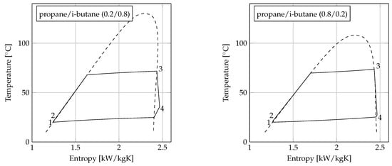
Figure 4.
-diagrams for the four ORC units using propane, i-butane, propane/i-butane (0.2/0.8), and propane/i-butane (0.8/0.2) with C.
The variation of and for the condensers are depicted in Figure 5. When the minimum pinch point temperature difference was the same for the pure fluids and the mixtures, the heat transfer equipment used for mixture condensation was associated with larger values of and smaller values of mean temperature difference. The performance comparison was therefore affected by whether the fluids were compared based on the same values of the minimum pinch point temperature difference, mean temperature difference or .
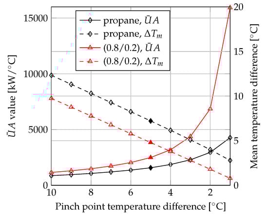
Figure 5.
Condenser and mean temperature difference versus pinch point temperature difference.
3.1.2. Mean Temperature Difference Based Comparison
The plot depicted in Figure 6 is generated by exchanging the minimum condenser pinch point temperature difference represented on the horizontal axis in Figure 3 with the mean temperature difference. Note that the optimized solutions displayed in Figure 3 and Figure 6 are the same. For each fluid, the left most points in Figure 6 correspond to the solutions with a minimum pinch point temperature difference in the condenser of 10 C, while the right most points correspond to the optimized solutions with minimum pinch point temperature difference values of 1 C. The filled marker represent the solutions with a minimum pinch point temperature difference of 5 C.
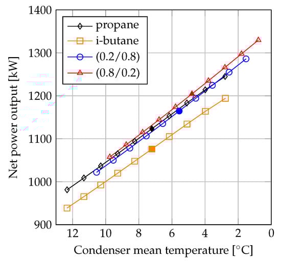
Figure 6.
Net power output as a function of condenser mean temperature difference.
For all fluids plotted in Figure 6, the relationship between the mean temperature difference and the net power output were approximately linear. This was also the case when the fluids were compared based on the same values of condenser pinch points. However, when compared based on the mean temperature differences, the curves for the pure fluids and the mixtures were displaced relative to each other. Generally, the mixtures achieved mean temperature differences that were similar to the pinch point temperature differences, while the pure fluids had mean temperature differences that were 1.5–3 C higher than the pinch points. This means that the performance improvement obtained by mixtures was rated less when the comparison was based on the same values of mean temperature differences than on the same values of minimum pinch point temperature differences. The results shown in Figure 6 suggest that the performance of propane was higher than that of propane/i-butane (0.2/0.8) for mean temperature differences higher than 3 C, whereas propane/i-butane (0.2/0.8) reached higher net power outputs than those of propane for all values of the condenser pinch point temperature difference in the pinch point based comparison (see Figure 3).
A comparison of the condensation processes for propane and propane/i-butane (0.2/0.8) is illustrated in the -diagrams (heat transfer rate versus temperature diagrams) depicted in Figure 7 and Figure 8. Figure 7 displays the comparison based on equal values of minimum pinch point temperature differences (C). The condensation process of propane is displayed as a horizontal line, since the optimum solution resulted in condensation from saturated vapor to saturated liquid. The optimum solution for propane/i-butane (0.2/0.8) involved 10 C of desuperheating. Disregarding the desuperheating process, the condensation process for propane/i-butane (0.2/0.8) was carried out at a lower temperature than the condensation of propane, resulting in a lower mean temperature for the mixture. Due to the match between the temperature glide of the mixture and the temperature increase of the coolant, the minimum pinch point temperature difference value could be achieved throughout most of the condensation process. This resulted in dissimilar mean temperatures for the pure fluid and the mixture. The mean temperature was C for propane, while it ess C for the mixture. When the pinch point temperature difference of propane/i-butane (0.2/0.8) was increased by 2 C, the mean temperatures of the two fluids were equal. This situation is displayed in Figure 8. When C for both fluids, the temperature difference between the coolant and the condensing working fluid was lowest for the mixture in the left half of the -diagram (from 0% to 50% heat transfer rate), while it was lowest for propane in the remaining part of the diagram (from 50% to 100% heat transfer rate).
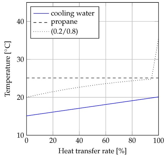
Figure 7.
-diagram of condensation when C for propane and propane/i-butane (0.2/0.8).
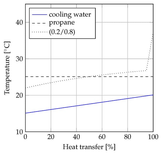
Figure 8.
-diagram of condensation when C for propane and propane/i-butane (0.2/0.8).
3.1.3. Value Based Comparison
The plot depicted in Figure 9 displays the comparison of propane, i-butane, propane/i-butane (0.2/0.8), and propane/i-butane (0.8/0.2). Figure 9 is an alternative representation of the results presented in Figure 3 and Figure 6. Essentially, the difference between Figure 3 and Figure 9 is that the net power outputs are plotted as a function of instead of minimum pinch point temperature differences. The left most values (lowest and net power output) plotted in Figure 9 thereby correspond to the solutions with minimum pinch point temperature difference values of 10 C, while the right most values (highest and net power output) correspond to the solutions with minimum pinch point temperature values of 1 C. Note that the solutions with 1 C minimum pinch point temperature difference for the mixtures are outside the boundaries of the plot. The filled markers correspond to the solutions with minimum pinch point temperature differences of 5 C.
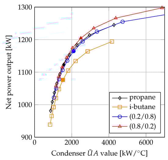
Figure 9.
Net power output as a function of condenser .
In the comparison between propane and propane/i-butane (0.2/0.8), propane achieved the highest performance for values below 4000 kW/C. The plots in Figure 9 suggest that the benefits of using mixtures were highest when the value of for the condenser was high. Furthermore, by comparing the net power outputs of the fluids based on the same values of the condenser , the increase in net power output was lower compared to the case when the net power outputs were compared based on the same minimum pinch point temperature differences. For example, the net power output of the mixture propane/i-butane (0.8/0.2) was 7.0% higher compared to propane for condenser minimum pinch point temperature differences of 3 C. Simultaneously, the value of the condenser was 91% higher for the mixture compared to propane. When the net power outputs were compared based on condenser values of 4300 kW/C (corresponding to C for the mixture and C for propane) the net power output of the mixture was 1.7% larger compared to that of propane. Comparing the fluids based on the same values was similar to the comparison based on equal mean temperature differences, since the variation in heat transfer rate was insignificant. These results indicate that the comparison based on the same minimum pinch point temperature differences resulted in an optimistic estimation of the thermodynamic benefit of using zeotropic mixtures, while the comparisons based on the same values and mean temperature difference resulted in conservative estimations of the benefits of using zeotropic mixtures.
3.1.4. Heat Transfer Area Based Comparison
Figure 10 shows the results of the fluid comparison when the fluids are rated on equal values of heat transfer area for the condenser. Similar to Figure 9, the plots in Figure 10 were generated based on the optimized solutions from Figure 3. The heat transfer areas were calculated based on the outputs (pressures, temperatures and mass flow rates) from the thermodynamic ORC process model by using the shell-and-tube heat exchanger model with conditions listed in Table 3. For each fluid, the lowest condenser areas in Figure 10 correspond to minimum pinch point temperature difference values of 10 C, while the highest condenser areas correspond to minimum pinch point temperature values of 1 C. The filled markers denote the solutions with a minimum pinch point temperature difference of 5 C.
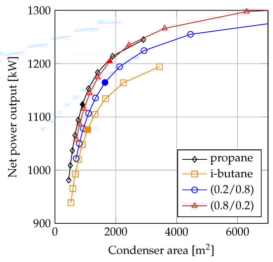
Figure 10.
Net power output as a function of condenser heat transfer area.
By comparing Figure 9 and Figure 10, the influence of the variation in can be observed. The heat transfer performance of propane was higher than that of i-butane. Furthermore, the overall heat transfer coefficient of propane was also larger than those of the mixtures. In the comparisons depicted in Figure 10, the larger heat transfer coefficient of propane increased the feasibility of this fluid compared to the value based method presented in Figure 9.
At condenser areas below 2000 m, propane was the highest performing fluid. At around 2000 m, there was a crossing of the curves for propane and propane/i-butane (0.8/0.2), and at higher condenser areas the (0.8/0.2) mixture achieved the highest net power outputs. The curve crossing occurred where the minimum pinch point temperature difference in the condensers was around 2 C for propane and 5 C for the mixture.
3.2. Fluid Performance Ranking
In this section, it is demonstrated how the outcome of a fluid performance ranking can be affected by the employed modeling method. The demonstration is based on the fluid selection study presented by Andreasen et al. [10] for a 120 C liquid water heat source, and the fluids considered for comparison are the 30 optimum fluids identified in that study. In the present study, the net power output of the ORC unit was maximized for each of the 30 fluids by employing the modeling conditions listed in Table 1. Supercritical pressures were allowed and the maximum pressure was limited to 100 bar. The high pressure in the system was limited to be below 80% of the critical pressure for subcritical systems and above 120% of the critical pressure for transcritical systems. For transcritical ORC solutions, the degree of superheating was replaced by the temperature difference between the expander inlet temperature and the critical temperature as decision variable which was varied in the range from 0 C to 100 C. For mixtures, the composition was optimized.
The ranking of the 30 working fluids based on fixed minimum pinch point temperature differences of C and C is listed in Table 4. The ranking was essentially the same as that presented by Andreasen et al. [10] except from the definition of the expander efficiency, which Andreasen et al. [10] based on a polytropic efficiency of 0.8, while an isentropic efficiency of 0.8 was employed in the present study. Moreover, the pressure constraints for subcritical and transcritical ORC solutions were not employed by Andreasen et al. [10]. This resulted in small variations in the fluid ranking compared to the previous results.
Table 4.
Fluid selection and optimization based on fixed values of the minimum pinch point temperature difference C and C.
Table 5 lists the ranking of the 30 fluids when based on a fixed value of kW/C. This value is the sum of the primary heat exchanger and condenser values for R218 in Table 4. The distribution of the total value between the primary heat exchanger and condenser was included as a decision variable. The optimization of the distribution enabled the power output of the ORC unit with R218 to increase from 1444 kW to 1460 kW. Despite this increase, the fluid was not ranked as the best performing fluid when the same value of was assumed for all fluids. Instead, the results suggest that R143a was the highest performing fluid due to an increase in net power output from 1361 kW to 1521 kW. This large increase was due to the relatively low value of resulting from the minimum pinch point temperature difference based optimization (see Table 4). When comparing the net power output and value of R218 and R143a in Table 4, R218 reached 6% higher net power output with 22% higher . The minimum pinch point temperature difference based method resulted in large differences in the requirement for the heat exchangers. When rated based on the value method, the differences due to variations in the values were eliminated, which enabled a fairer comparison of the fluids. The fluids R227ea, R1234yf and propylene also experienced a large increase in the ranking when rated on the value based method rather than the minimum pinch point temperature difference based method.
Table 5.
Fluid selection and optimization based on fixed values of kW/C.
Generally, the results indicate that, when the fluid ranking was based on equal values of , the pure fluids performed better relative to the zeotropic mixtures than when the performance comparison was based on equal values of the minimum pinch point temperature difference. In the minimum pinch point temperature difference based comparison, 19 out of the 30 fluids were zeotropic mixtures (including the predefined mixture R422A). In this case, the zeotropic mixtures enabled up to 13.6% higher performance compared to the best pure fluid in each mixture. In the based comparison, only 12 fluids were zeotropic mixtures, since the composition of seven mixtures converged to 0% or 100% mole fraction. In this case, the performance increase of the zeotropic mixtures compared to the best pure fluid in each mixture was below 2.6%. High performance was reached for the transcritical mixture ethane/propane in both fluid rankings, but the composition changed from 88.3% (in Table 4) to 3.73% (in Table 5). The mixtures propane/butane, propane/i-butane, propane/pentane, propane/i-pentane and propane/hexane did not reach higher net power output than pure propane. It is also worth noting that, although ethane as a pure fluid reached the lowest net power output of the 30 fluids, it was possible to reach higher net power outputs than propane, butane, i-butane, pentane, and i-pentane by mixing small amounts of ethane in these fluids. The propane/i-butane mixture, which was analyzed thoroughly (see Section 3.1), did not reach higher performance than pure propane.
Moreover, when the fluid ranking was based on equal values of the minimum pinch point temperature difference, 17 out of the 30 fluids were transcritical, but, in the fluid ranking based on equal values of , only seven fluids were transcritical. The highest net power output was still achieved with transcritical ORC units, however the relative difference in net power output of the highest performing subcritical compared to the highest performing transcritical unit was reduced from 18.8% (R227ea compared to R218 in Table 4) to 1.1% (R227ea compared to R143a in Table 5). This indicates that the method assuming the same minimum pinch point temperature differences for all fluids resulted in optimistic performance estimations of the thermodynamic benefits of using transcritical ORC units and/or zeotropic mixtures, while the method assuming the same total value resulted in a conservative estimations.
3.3. Assessment of Modeling Methods
The use of zeotropic mixtures provides the flexibility of adjusting the temperature profile of evaporation and condensation to obtain optimal alignment with the temperature profiles of sensible heat sources and sinks. This has an effect on the temperature difference between the heat exchanging fluid streams throughout the primary heat exchanger and the condenser. By basing the comparison of pure fluids and mixtures on equal values of the minimum pinch point temperature difference, there is no distinguishing between solutions where the minimum temperature difference value is reached at a single location in the heat exchanger (for example in case of pure fluids) and solutions where the temperature difference is close to the minimum value throughout the heat exchanger (in case of temperature profile matching) (see Figure 7). However, as demonstrated in Section 3.1, these two situations can result in very different mean temperatures and values. Ultimately, when comparing pure fluids and zeotropic mixtures based on equal values of minimum pinch point temperature difference, the zeotropic mixtures benefit from reduced irreversibilities in the heat transfer processes due to temperature profile matching. However, the additional cost related to the larger heat transfer equipment required for transferring the heat across a lower mean temperature difference is unaccounted for. Thereby, the estimation of the benefit of temperature profile matching is deemed to be optimistic when the comparison is based on equal values of minimum pinch point temperature differences, since the ORC unit employing the zeotropic mixtures are provided with the additional benefit of having heat exchangers with larger thermal capacity (larger and lower mean temperature difference). Using this thermodynamic modeling approach for comparing the performance of pure fluids and zeotropic mixtures there is a risk of overestimating the benefits of zeotropic mixtures, which might not be representative of the actual performance difference when the cost of heat exchangers are taken into account in subsequent thermoeconomic analyses.
By use of alternative modeling methods, it is possible, with limited additional modeling effort, to take differences in mean temperature differences or values into account. The added modeling complexity solely consists of discretizing the heat exchangers in a suitable number of control volumes, which enables to calculate the values and mean temperature differences, and defining limiting values for either of them. In many situations it is even required to discretize the heat transfer process for identifying the location of the minimum pinch point temperature difference, for example when the temperature profile of the mixture is highly curved, or when the high pressure is supercritical or slightly below the critical pressure. It is beneficial to specify limits for the mean temperature difference or the value of the heat exchangers rather than for the minimum pinch point temperature difference, since the mean temperature difference and the value take the complete heat transfer process into account and are therefore more indicative of the heat transfer surface area and thereby the cost of the heat exchanger. The use of the methods assuming either the same mean temperature difference or the same values for pure fluids and zeotropic mixtures, is deemed to result in conservative estimations of the thermodynamic performance benefit of using zeotropic mixtures.
Defining a constraint based on the mean temperature difference is beneficial in the sense that it is conceptually similar to the minimum pinch point temperature difference and it is therefore easier to define suitable limiting values. Defining heat exchanger constraints based on values provides an additional option of optimizing the distribution of to each of the heat exchangers by defining a limit for the total ORC unit (sum of for all heat exchangers in the unit). The drawback of defining constraints based on values is that the value depends on the capacity of the system, i.e., the net power output and heat transferred in the process. One way of addressing this issue is to define a base case fluid for which the heat exchanger minimum pinch point temperature differences are fixed at reasonable values. The values of the heat exchangers for the base case solution can then be used as limiting values for the remaining simulations. The use of methods fixing the mean temperature differences or values of heat exchangers does not account for differences in heat transfer coefficients. Such differences can be accounted for by including heat exchanger models in the optimization framework for estimation of heat transfer areas. However, this requires the use of heat transfer correlations which adds to the model complexity and computational time required for the simulations. In relation to fluid screening studies, it is desirable to limit the computational time of the model when many fluids are evaluated. An overview of the method assessment is shown in Table 6.
Table 6.
Method assessment overview.
The thermodynamic modeling methods discussed in this paper do not account for effects of fluid properties on the design, efficiency and cost of the ORC expander. Such aspects are essential when selecting a fluid for an ORC unit. Astolfi et al. [45], Martelli et al. [46], and Meroni et al. [47] provided methods for including axial turbine design aspects in the framework of thermodynamic and thermoeconomic ORC process optimizations. Such methods are relevant to combine with the methods discussed in the present paper for preliminary design and optimization of ORC systems.
3.4. Feasibility of Using Zeotropic Mixtures
Traditionally, the primary reason for using zeotropic mixtures as working fluids in ORC power systems is to utilize the temperature glide of phase change for temperature profile matching with sensible heat sources and sinks, with the aim of reducing the irreversibilities of the heat transfer processes. As indicated in the fluid comparison based on equal heat transfer area (see Figure 10), those benefits are highest when the heat transfer area is high. In the theoretical case of infinitely large counter-flow heat exchangers, it is possible for mixtures to reach higher capacities (lower mean temperature differences and higher ) than pure fluids, since the temperature profiles achieve a better match with the sensible heat source and sink in the primary heat exchanger and the condenser. On the other hand, when the heat exchangers are small, the temperature differences in the heat exchangers are large and the values are small. In this case, the performance increase due to the better temperature match achieved with zeotropic mixtures is limited and tends to be overcompensated by the degradation in heat transfer coefficient, as demonstrated in Section 3.1.4. This observation indicates that zeotropic mixtures are more likely to be economically feasible compared to pure fluids in applications where it pays off to invest in large heat exchangers. This is the case in geothermal applications, where a large investment is required for establishing the geothermal well. Astolfi et al. [45] demonstrated how their thermoeconomic optimization results for pure fluids in an ORC unit designed for utilizing geothermal heat, was affected by the investment required for the geothermal well. A variation of the geothermal well cost from zero to 12 M€ resulted in an increase of the ORC unit cost (power block only) from 3.03 M€ to 8.57 M€, and a reduction of the minimum pinch point temperature difference of the condenser from 2.5 C to 0.43 C. Similarly, it is more likely that zeotropic mixtures achieve higher economic performance than pure fluids, when the cost of the heat exchangers is low.
It is also worthwhile considering zeotropic mixtures for other reasons than the temperature profile matching capabilities. By including zeotropic mixtures in the fluid screening, the number of considered working fluids is larger, and it is more likely to identify fluids with desirable properties considering multiple criteria such as thermodynamic performance, environmental friendliness, safety and cost. For example, the high flammability of hydrocarbons could be reduced by adding a non-flammable fluid [48,49]. Fluids which result in high process pressures could benefit from being mixed with a low pressure fluid. This could result in a reduction in piping and heat exchanger costs [25]. Additionally, for the same condenser bubble point (condensing fluid outlet temperature), it is possible for zeotropic mixtures to have a higher increase in the coolant temperature due to the temperature glide. For the same amount of heat transfer, the mass flow rate of cooling water can thereby be smaller for mixtures. This can result in lower size and cost for cooling water circulating pumps, and cooling towers [5].
3.5. Method Selection for Other Thermodynamic Processes
Temperature profile matching is not only utilized for zeotropic mixtures, but also for pure fluids where temperature profile matching in the preheater has been used for optimizing the ORC system performance [50,51]. In addition, the use of a recuperator can result in almost perfect alignment of the temperature profiles of the heated liquid and the cooled vapor [51]. In such situations, it is important to check that the mean temperature differences and the values do not get excessively low and high, respectively. In power cycle units where the pressure is supercritical, for example transcritical ORC units or supercritical CO units, temperature profile matching is possible in the heat transfer process between the hot fluid and the supercritical working fluid. When comparing such units with power cycle units using subcritical pressures it is also important to account for differences in mean temperature differences and values in order not to overestimate the performance of the units employing supercritical pressures (see also Section 3.2). Due to the curved temperature profile of the supercritical heating process it is necessary to discretize the heat exchanger for identifying the pinch point location. Thus, it is possible to define constraints on the mean temperature difference or values of the heat exchangers with limited additional effort compared to applying minimum pinch point temperature difference constraints.
The implementation of constraints on either mean temperature differences or values rather than minimum pinch point temperature differences, should also be considered for other power cycles utilizing zeotropic mixtures as working fluids. Examples of such cycles are the Kalina cycle using ammonia/water mixtures, and physical absorption cycles using lithium-bromide/water mixtures.
The alternative methods discussed in this paper are also useful in combination with computer aided molecular design (CAMD) [52,53,54], and continuous molecular targeting (CoMT) [55,56] methods, which consider the molecular optimization of the working fluid. In such optimization problems, the ORC process model is typically based on thermodynamics, since a full thermoeconomic model including heat exchanger sizing would be too extensive to implement at this stage. Although the CAMD and CoMT methods are able to identify thermodynamic optima, it is possible that the fluids designed are not thermoeconomically optimal. By using minimum pinch point temperature difference based models, there is a risk that benefits due to temperature profile matching is overestimated. It is therefore important to check whether there is a correlation between values or mean temperatures, with the performance ranking of the designed fluids. If this is the case, it is worthwhile considering implementation of constraints on mean temperature differences or values. Cignitti et al. [57] carried out a CAMD based optimization integrating ORC process and working fluid design, and found different optimum working fluids depending on whether the selected heat exchanger constraints were based on minimum pinch point temperature differences or values.
4. Conclusions
In this paper, four different methods for performance comparison of pure fluids and zeotropic mixtures in ORC systems were assessed. The methods were characterized by which modeling approach was used for representing the performance of the heat exchangers in the systems. The methods compared the net power output of the fluids based on either the same minimum pinch point temperature differences, the same mean temperature differences, the same values, or the same heat transfer areas for all fluids.
The comparison of propane, i-butane, propane/i-butane (0.2/0.8) and propane/i-butane (0.8/0.2) based on the same values of condenser pinch point temperature differences suggests that the highest net power outputs are achieved by the mixtures for all values of condenser pinch temperature difference. When compared based on the same values of condenser mean temperature differences or values, the results suggest that propane/i-butane (0.8/0.2) achieves the highest net power output. However, the mixture propane/i-butane (0.2/0.8) is outperformed by propane at condenser mean temperature differences above 3 C and values below 4000 kW/C. When comparing the net power outputs of the fluids based on the same condenser heat transfer areas, the highest performance is achieved by propane at heat transfer areas below 2000 m, while propane/i-butane (0.8/0.2) achieves the highest performance at heat transfer areas above 2000 m. In the heat transfer area based comparison, propane achieves higher net power outputs than propane/i-butane (0.2/0.8) for all considered values of the condenser heat transfer area. The results suggest that the fluid i-butane achieves the lowest net power outputs of the four fluids in all the considered cases.
A fluid performance ranking of 30 working fluids assuming the same minimum pinch point temperature differences for all fluids, indicates that the net power outputs of zeotropic mixtures are up to 13.6% higher compared to the best pure fluids in the mixtures. On the other hand, by assuming that the sum of the condenser and primary heat exchanger value is the same for all fluids, the results indicate that the net power outputs of zeotropic mixtures are only up to 2.56% higher compared to the best pure fluids in the mixtures. Similarly, the estimated performance benefit of using transcritical ORC units decreases from 18.8% in the minimum pinch point temperature difference based comparison to 1.1% in the value based comparison.
The method assuming equal minimum pinch point temperature differences for all fluids was deemed to result in optimistic estimations of the benefits of using zeotropic mixtures, while the methods assuming equal mean temperature differences or values were deemed to result in conservative estimations. The method assuming equal heat transfer areas for all fluids was deemed too comprehensive for thermodynamic optimization considering modeling complexity and computational time. This indicates that it is beneficial to use the method assuming equal minimum pinch point temperature differences and the method assuming equal values (or mean temperature differences) concurrently in preliminary fluid selection, since they result in different conclusions regarding the thermodynamic performance of working fluids.
Relevant future work within this research topic could comprise an economic optimization of an ORC system considering a group of selected working fluids. By carrying out the working fluid selection for the economic analysis based on two or more of the thermodynamic methods assessed in the present paper, it is possible to judge which of the methods identifies the more economically beneficial working fluids.
Author Contributions
Conceptualization, J.G.A., M.R.K. and F.H.; Formal analysis, J.G.A.; Funding acquisition, F.H.; Investigation, J.G.A.; Methodology, J.G.A., M.R.K. and F.H.; Project administration, F.H.; Supervision, M.R.K. and F.H.; Validation, J.G.A. and M.R.K.; Writing—original draft, J.G.A.; and Writing—review and editing, M.R.K. and F.H.
Funding
This research was funded by Innovationsfonden, The Danish Council for Strategic Research in Sustainable Energy and Environment project ID: 1305-00036B.
Acknowledgments
The work presented in this paper was conducted within the frame of the THERMCYC project (“Advanced thermodynamic cycles utilising low-temperature heat sources”, project ID: 1305-00036B; see www.thermcyc.mek.dtu.dk) funded by Innovationsfonden, The Danish Council for Strategic Research in Sustainable Energy and Environment. The financial support is gratefully acknowledged.
Conflicts of Interest
The authors declare no conflict of interest.
Nomenclature
| Abbreviations | |
| CAMD | Computer aided molecular design |
| CoMT | Continuous molecular targeting |
| ORC | Organic Rankine cycle |
| Greek symbols | |
| Convective heat transfer coefficient, (kW/m C) | |
| Difference | |
| Efficiency, (%) | |
| Thermal conductivity, (kW/mC) | |
| Symbols | |
| A | Area, (m) |
| d | Diameter, (m) |
| h | Specific enthalpy, (kJ/kg) |
| L | Tube length, (m) |
| Length of baffle cut, (m) | |
| Mass flow rate, (kg/s) | |
| n | Number of control volumes, (-) |
| Number of tubes, (-) | |
| P | Pressure, (bar) |
| Tube pitch, (m) | |
| Heat transfer rate, (kW) | |
| T | Temperature, (C) |
| Average overall heat transfer coefficient, (kW/m C) | |
| Mechanical power, (kW) | |
| X | Mole fraction, (-) |
| Subscripts and superscripts | |
| c | Cold |
| cond | Condenser |
| crit | Critical |
| g | Glide of condensation |
| hf | Hot fluid |
| i | Input |
| in | Inner |
| j | Control volume counter |
| lm | Log mean |
| m | Mean |
| mix | Mixture |
| net | Net |
| o | Out |
| ou | Outer |
| pp | Pinch point |
| PrHE | Primary heat exchanger |
| pure | Pure fluid |
| r | Relative |
| sc | Subcritical |
| tc | Transcritical |
| tot | Total |
| wf | Working fluid |
Appendix A
Table A1 displays the variation in net power output, condenser mean temperature difference, condenser values, and condenser areas as functions of the condenser pinch point temperature difference for the working fluids propane, i-butane, propane/i-butane (0.2/0.8) and propane/i-butane (0.8/0.2). The data are plotted in Figure 3, Figure 5, Figure 6, Figure 9, and Figure 10.
Table A1.
Variation of net power output (), condenser mean temperature difference (), condenser values (), and condenser areas () as functions of the condenser pinch point temperature difference () for propane, i-butane and the mixtures propane/i-butane (0.2/0.8) and propane/i-butane (0.8/0.2).
Table A1.
Variation of net power output (), condenser mean temperature difference (), condenser values (), and condenser areas () as functions of the condenser pinch point temperature difference () for propane, i-butane and the mixtures propane/i-butane (0.2/0.8) and propane/i-butane (0.8/0.2).
| [C] | 10 | 9 | 8 | 7 | 6 | 5 | 4 | 3 | 2 | 1 | |
|---|---|---|---|---|---|---|---|---|---|---|---|
| [kW] | propane | 981 | 1009 | 1037 | 1065 | 1094 | 1123 | 1153 | 1183 | 1214 | 1245 |
| i-butane | 939 | 965 | 992 | 1020 | 1048 | 1076 | 1105 | 1134 | 1164 | 1194 | |
| (0.2/0.8) | 1022 | 1050 | 1078 | 1107 | 1135 | 1165 | 1194 | 1224 | 1255 | 1286 | |
| (0.8/0.2) | 1058 | 1086 | 1115 | 1144 | 1174 | 1204 | 1235 | 1266 | 1298 | 1330 | |
| [C] | propane | 12.3 | 11.3 | 10.3 | 9.3 | 8.2 | 7.2 | 6.2 | 5.1 | 4.0 | 2.8 |
| i-butane | 12.3 | 11.3 | 10.3 | 9.3 | 8.2 | 7.2 | 6.2 | 5.1 | 4.0 | 2.8 | |
| (0.2/0.8) | 10.6 | 9.5 | 8.5 | 7.5 | 6.6 | 5.6 | 4.6 | 3.6 | 2.5 | 1.5 | |
| (0.8/0.2) | 9.8 | 8.8 | 7.8 | 6.8 | 5.8 | 4.8 | 3.8 | 2.8 | 1.8 | 0.8 | |
| [kW/C] | propane | 865 | 957 | 1065 | 1200 | 1362 | 1572 | 1865 | 2286 | 2953 | 4273 |
| i-butane | 835 | 924 | 1025 | 1154 | 1315 | 1527 | 1808 | 2207 | 2858 | 4164 | |
| (0.2/0.8) | 1041 | 1163 | 1319 | 1511 | 1761 | 2100 | 2590 | 3357 | 4740 | 8008 | |
| (0.8/0.2) | 1155 | 1302 | 1486 | 1726 | 2041 | 2492 | 3185 | 4370 | 6859 | 15925 | |
| [m] | propane | 454 | 508 | 575 | 660 | 765 | 905 | 1105 | 1402 | 1892 | 2909 |
| i-butane | 527 | 591 | 672 | 773 | 902 | 1078 | 1317 | 1664 | 2249 | 3439 | |
| (0.2/0.8) | 701 | 803 | 936 | 1105 | 1333 | 1645 | 2128 | 2930 | 4455 | 8426 | |
| (0.8/0.2) | 705 | 815 | 957 | 1149 | 1412 | 1806 | 2433 | 3603 | 6298 | 17671 |
References
- Tchanche, B.F.; Lambrinos, G.; Frangoudakis, A.; Papadakis, G. Low-grade heat conversion into power using organic Rankine cycles—A review of various applications. Renew. Sustain. Energy Rev. 2011, 15, 3963–3979. [Google Scholar] [CrossRef]
- Quoilin, S.; van den Broek, M.; Declaye, S.; Dewallef, P.; Lemort, V. Techno-economic survey of Organic Rankine Cycle (ORC) systems. Renew. Sustain. Energy Rev. 2013, 22, 168–186. [Google Scholar] [CrossRef]
- Colonna, P.; Casati, E.; Trapp, C.; Mathijssen, T.; Larjola, J.; Turunen-Saaresti, T.; Uusitalo, A. Organic Rankine Cycle Power Systems: From the Concept to Current Technology, Applications, and an Outlook to the Future. J. Eng. Gas Turbines Power 2015, 137, 100801. [Google Scholar] [CrossRef]
- Andreasen, J.; Meroni, A.; Haglind, F. A Comparison of Organic and Steam Rankine Cycle Power Systems for Waste Heat Recovery on Large Ships. Energies 2017, 10, 547. [Google Scholar] [CrossRef]
- Demuth, O.; Kochan, R.J. Analyses of Mixed Hydrocarbon Binary Thermodynamic Cycles For Moderate Temperature Geothermal Resources Using Regeneration Techniques; Technical Report; US Department of Energy: Idaho Falls, ID, USA, December 1981.
- Angelino, G.; Colonna, P. Multicomponent working fluids for organic Rankine cycles (ORCs). Energy 1998, 23, 449–463. [Google Scholar] [CrossRef]
- Modi, A.; Haglind, F. A review of recent research on the use of zeotropic mixtures in power generation systems. Energy Convers. Manag. 2017, 138, 603–626. [Google Scholar] [CrossRef]
- Radermacher, R. Thermodynamic and heat transfer implications of working fluid mixtures in Rankine cycles. Int. J. Heat Fluid Flow 1989, 10, 90–102. [Google Scholar] [CrossRef]
- Heberle, F.; Preißinger, M.; Brüggemann, D. Zeotropic mixtures as working fluids in Organic Rankine Cycles for low-enthalpy geothermal resources. Renew. Energy 2012, 37, 364–370. [Google Scholar] [CrossRef]
- Andreasen, J.G.; Larsen, U.; Knudsen, T.; Pierobon, L.; Haglind, F. Selection and optimization of pure and mixed working fluids for low grade heat utilization using organic Rankine cycles. Energy 2014, 73, 204–213. [Google Scholar] [CrossRef]
- Lecompte, S.; Ameel, B.; Ziviani, D.; van den Broek, M.; De Paepe, M. Exergy analysis of zeotropic mixtures as working fluids in Organic Rankine Cycles. Energy Convers. Manag. 2014, 85, 727–739. [Google Scholar] [CrossRef]
- Braimakis, K.; Preißinger, M.; Brüggemann, D.; Karellas, S.; Panopoulos, K. Low grade waste heat recovery with subcritical and supercritical Organic Rankine Cycle based on natural refrigerants and their binary mixtures. Energy 2015, 88, 80–92. [Google Scholar] [CrossRef]
- Trapp, C.; Colonna, P. Efficiency Improvement in Precombustion CO2 Removal Units with a Waste-Heat Recovery ORC Power Plant. J. Eng. Gas Turbines Power 2013, 135, 042311. [Google Scholar] [CrossRef]
- Weith, T.; Heberle, F.; Preißinger, M.; Brüggemann, D. Performance of Siloxane Mixtures in a High-Temperature Organic Rankine Cycle Considering the Heat Transfer Characteristics during Evaporation. Energies 2014, 7, 5548–5565. [Google Scholar] [CrossRef]
- Baik, Y.J.; Kim, M.; Chang, K.C.; Lee, Y.S.; Yoon, H.K. A comparative study of power optimization in low-temperature geothermal heat source driven R125 transcritical cycle and HFC organic Rankine cycles. Renew. Energy 2013, 54, 78–84. [Google Scholar] [CrossRef]
- Baik, Y.J.; Kim, M.; Chang, K.C.; Lee, Y.S.; Yoon, H.K. Power enhancement potential of a mixture transcritical cycle for a low-temperature geothermal power generation. Energy 2012, 47, 70–76. [Google Scholar] [CrossRef]
- Bombarda, P.; Invernizzi, C.M.; Pietra, C. Heat recovery from Diesel engines: A thermodynamic comparison between Kalina and ORC cycles. Appl. Therm. Eng. 2010, 30, 212–219. [Google Scholar] [CrossRef]
- Le, V.L.; Kheiri, A.; Feidt, M.; Pelloux-Prayer, S. Thermodynamic and economic optimizations of a waste heat to power plant driven by a subcritical ORC (Organic Rankine Cycle) using pure or zeotropic working fluid. Energy 2014, 78, 622–638. [Google Scholar] [CrossRef]
- Feng, Y.; Hung, T.; Zhang, Y.; Li, B.; Yang, J.; Shi, Y. Performance comparison of low-grade ORCs (organic Rankine cycles) using R245fa, pentane and their mixtures based on the thermoeconomic multi-objective optimization and decision makings. Energy 2015, 93, 2018–2029. [Google Scholar] [CrossRef]
- Feng, Y.; Hung, T.; Greg, K.; Zhang, Y.; Li, B.; Yang, J. Thermoeconomic comparison between pure and mixture working fluids of organic Rankine cycles (ORCs) for low temperature waste heat recovery. Energy Convers. Manag. 2015, 106, 859–872. [Google Scholar] [CrossRef]
- Heberle, F.; Brüggemann, D. Thermo-Economic Evaluation of Organic Rankine Cycles for Geothermal Power Generation Using Zeotropic Mixtures. Energies 2015, 8, 2097–2124. [Google Scholar] [CrossRef]
- Oyewunmi, O.; Markides, C. Thermo-Economic and Heat Transfer Optimization of Working-Fluid Mixtures in a Low-Temperature Organic Rankine Cycle System. Energies 2016, 9, 448. [Google Scholar] [CrossRef]
- Heberle, F.; Brüggemann, D. Thermo-Economic Analysis of Zeotropic Mixtures and Pure Working Fluids in Organic Rankine Cycles for Waste Heat Recovery. Energies 2016, 9, 226. [Google Scholar] [CrossRef]
- Imran, M.; Usman, M.; Lee, D.H.; Park, B.S. Thermoeconomic analysis of organic Rankine cycle using zeotropic mixtures. In Proceedings of the 3rd International Seminar on ORC Power Systems, Brussels, Belgium, 12–14 October 2015; p. 161. [Google Scholar]
- Andreasen, J.; Kærn, M.; Pierobon, L.; Larsen, U.; Haglind, F. Multi-Objective Optimization of Organic Rankine Cycle Power Plants Using Pure and Mixed Working Fluids. Energies 2016, 9, 322. [Google Scholar] [CrossRef]
- Mclinden, M.O.; Radermacher, R. Methods for comparing the performance of pure and mixed refrigerants in the vapour compression cycle. Int. J. Refrig. 1987, 10, 318–325. [Google Scholar] [CrossRef]
- Högberg, M.; Vamling, L.; Berntsson, T. Calculation methods for comparing the performance of pure and mixed working fluids in heat pump applications. Int. J. Refrig. 1993, 16, 403–413. [Google Scholar] [CrossRef]
- Mathworks. Matlab 2018b Documentation; Technical Report; Mathworks: Natick, MA, USA, 2018. [Google Scholar]
- Lemmon, E.W.; Huber, M.; McLinden, M. NIST Standard Reference Database 23: Reference Fluid Thermodynamic and Transport Properties-REFPROP; version 9.0; National Institute of Standards and Technology, Standard Reference Data Program: Gaithersburg, MD, USA, 2010.
- Bell, I.H.; Wronski, J.; Quoilin, S.; Lemort, V. Pure and Pseudo-pure Fluid Thermophysical Property Evaluation and the Open-Source Thermophysical Property Library CoolProp. Ind. Eng. Chem. Res. 2014, 53, 2498–2508. [Google Scholar] [CrossRef]
- Shah, R.K.; Sekulić, D.P. Fundamentals of Heat Exchanger Design; John Wiley & Sons, Inc.: Hoboken, NJ, USA, 2003. [Google Scholar] [CrossRef]
- Coulson, J.; Richardson, J.; Backhurst, J. Coulson and Richardson’s Chemical Engineering; Butterworth-Heinemann: Oxford, UK, 1999. [Google Scholar]
- Walraven, D.; Laenen, B.; D’haeseleer, W. Optimum configuration of shell-and-tube heat exchangers for the use in low-temperature organic Rankine cycles. Energy Convers. Manag. 2014, 83, 177–187. [Google Scholar] [CrossRef]
- Kærn, M.R.; Modi, A.; Jensen, J.K.; Haglind, F. An assessment of transport property estimation methods for ammonia-water mixtures and their influence on heat exchanger size. Int. J. Thermophys. 2015, 36, 1468–1497. [Google Scholar] [CrossRef]
- Bell, K.J. Final Report of the Cooperative Research Program on Shell-and-Tube Heat Exchangers; Technical Report; University of Delaware: Newark, DE, USA, 1963. [Google Scholar]
- Bell, K.J. Delaware method for shell design. In Heat Transfer Equipment Design; Shah, R.K., Subbarao, E.C., Mashelkar, R.A., Eds.; Hemisphere Publishing: Washington, DC, USA, 1988. [Google Scholar]
- Taborek, J. Shell-and-tube heat exchangers: Single phase flow. In Handbook of Heat Exchanger Design; Hewitt, G.F., Ed.; Begell House: New York, NY, USA, 1998; Chapter 3. [Google Scholar]
- Shah, M.M. An Improved and Extended General Correlation for Heat Transfer During Condensation in Plain Tubes. HVAC&R Res. 2009, 15, 889–913. [Google Scholar] [CrossRef]
- Gnielinski, V. New equation for heat and mass transfer in turbulent pipe and channel flow. Int. Chem. Eng. 1976, 16, 359–368. [Google Scholar]
- Petukhov, B. Heat Transfer and Friction in Turbulent Pipe Flow with Variable Physical Properties. Adv. Heat Transf. 1970, 6, 503–564. [Google Scholar] [CrossRef]
- Bell, K.; Ghaly, M. An approximate generalized design method for multicomponent/partial condenser. AIChE Symp. Ser. 1973, 69, 72–79. [Google Scholar]
- Blasius, H. Das Ähnlichkeitsgesetz bei Reibungsvorgängen in Flüssigkeiten. In Mitteilungen über Forschungsarbeiten auf dem Gebiete des Ingenieurwesens 131; Springer: Berlin, Germany, 1913. [Google Scholar]
- Müller-Steinhagen, H.; Heck, K. A simple friction pressure drop correlation for two-phase flow in pipes. Chem. Eng. Process. Process Intensif. 1986, 20, 297–308. [Google Scholar] [CrossRef]
- Martin, H. The generalized Lévêque equation and its practical use for the prediction of heat and mass transfer rates from pressure drop. Chem. Eng. Sci. 2002, 57, 3217–3223. [Google Scholar] [CrossRef]
- Astolfi, M.; Romano, M.C.; Bombarda, P.; Macchi, E. Binary ORC (Organic Rankine Cycles) power plants for the exploitation of medium-low temperature geothermal sources—Part B: Techno-economic optimization. Energy 2014, 66, 435–446. [Google Scholar] [CrossRef]
- Martelli, E.; Capra, F.; Consonni, S. Numerical optimization of Combined Heat and Power Organic Rankine Cycles—Part A: Design optimization. Energy 2015, 90, 310–328. [Google Scholar] [CrossRef]
- Meroni, A.; Andreasen, J.G.; Persico, G.; Haglind, F. Optimization of organic Rankine cycle power systems considering multistage axial turbine design. Appl. Energy 2018, 209, 339–354. [Google Scholar] [CrossRef]
- Garg, P.; Kumar, P.; Srinivasan, K.; Dutta, P. Evaluation of isopentane, R-245fa and their mixtures as working fluids for organic Rankine cycles. Appl. Therm. Eng. 2013, 51, 292–300. [Google Scholar] [CrossRef]
- Garg, P.; Kumar, P.; Srinivasan, K.; Dutta, P. Evaluation of carbon dioxide blends with isopentane and propane as working fluids for organic Rankine cycles. Appl. Therm. Eng. 2013, 52, 439–448. [Google Scholar] [CrossRef]
- Liu, W.; Meinel, D.; Gleinser, M.; Wieland, C.; Spliethoff, H. Optimal Heat Source Temperature for thermodynamic optimization of sub-critical Organic Rankine Cycles. Energy 2015, 88, 897–906. [Google Scholar] [CrossRef]
- Andreasen, J.G.; Larsen, U.; Haglind, F. Design of organic Rankine cycles using a non-conventional optimization approach. In Proceedings of the ECOS 2015—the 28th International Conference on Efficiency, Cost, Optimization, Simulation and Environmental Impact of Energy Systems, Pau, France, 30 June–3 July 2015. [Google Scholar]
- Gani, R.; Nielsen, B.; Fredenslund, A. A group contribution approach to computer-aided molecular design. AIChE J. 1991, 37, 1318–1332. [Google Scholar] [CrossRef]
- Doucet, J.P.; Weber, J. Computer-Aided Molecular Design: Theory and Applications; Academic Press: Cambridge, MA, USA, 1996; p. 487. [Google Scholar]
- Papadopoulos, A.I.; Stijepovic, M.; Linke, P. On the systematic design and selection of optimal working fluids for Organic Rankine Cycles. Appl. Therm. Eng. 2010, 30, 760–769. [Google Scholar] [CrossRef]
- Lampe, M.; Stavrou, M.; Bücker, H.M.; Gross, J.; Bardow, A. Simultaneous Optimization of Working Fluid and Process for Organic Rankine Cycles Using PC-SAFT. Ind. Eng. Chem. Res. 2014, 53, 8821–8830. [Google Scholar] [CrossRef]
- Lampe, M.; Stavrou, M.; Schilling, J.; Sauer, E.; Gross, J.; Bardow, A. Computer-aided molecular design in the continuous-molecular targeting framework using group-contribution PC-SAFT. Comput. Chem. Eng. 2015, 81, 278–287. [Google Scholar] [CrossRef]
- Cignitti, S.; Andreasen, J.; Haglind, F.; Woodley, J.; Abildskov, J. Integrated working fluid-thermodynamic cycle design of organic Rankine cycle power systems for waste heat recovery. Appl. Energy 2017, 203. [Google Scholar] [CrossRef]
© 2019 by the authors. Licensee MDPI, Basel, Switzerland. This article is an open access article distributed under the terms and conditions of the Creative Commons Attribution (CC BY) license (http://creativecommons.org/licenses/by/4.0/).