Numerical Investigation of the Effect of Sudden Expansion Ratio of Solid Fuel Ramjet Combustor with Swirling Turbulent Reacting Flow

Abstract

In this paper, the effect of sudden expansion ratio of solid fuel ramjet (SFRJ) combustor is numerically investigated with swirl flow. A computational fluid dynamics (CFD) code is written in FORTRAN to simulate the combustion and flow patterns in the combustion chamber. The connected-pipe facility is used to perform the experiment with swirl, and high-density Polyethylene (HDPE) is used as the solid fuel. The investigation is performed with different sudden expansion ratios, in which the port and inlet diameters are independently varied. The results indicated that the self-sustained combustion of the SFRJ occurs around the reattachment point at first, and then the heat released in reattachment point is used to achieve the self-sustained combustion in the redevelopment zone. The average regression rate is proportional to the sudden expansion ratio for the cases with a fixed port diameter, which is mainly dominated by the enhancement of heat transfer in backward-facing step. However, the average regression rate is inversely proportional to the sudden expansion ratio for the cases with fixed inlet diameter, which is influenced by the heat transfer mechanism of developed turbulent flow in the redevelopment zone.

1. Introduction

Nowadays, solid fuel ramjet (SFRJ) has been widely used and researched in the military and aerospace fields, due to the advantages of simple structure, high reliability, and easy long-term storage. Thus, how to improve combustion performance is a hotspot of current researches. As can be seen from previous researches, the combustion performance of SFRJ could be highly determined by the regression rate, and it is easily influenced by the geometry of SFRJ combustor.

The regression rate and flow field characteristics of SFRJ and scramjets has been extensively investigated with experimental and theoretical studies. An experimental investigation on SFRJ is performed by Schulte [1], with different altitudes, flight speeds, and mass fluxes of in-coming air, to determine the fuel regression behavior. Polyethylene (PE) was used as the standard fuel. The results show that decreasing the port diameter, chamber pressure, and inlet temperature will increase the regression rate. Gany et al. [2] investigated the combustion that is affected by the geometry of Polymethylmethacrylate (PMMA) fueled SFRJ. The research founded that the local regression rate could be sensitive to the local convective heat flux and it was significantly affected by the port diameter. Ferreira et al. conducted experimental research on Polyethylene (PE) [3], at which the port diameter is varied from 20 mm to 45 mm. They found that changing port diameter has a significant effect on the regression rate. Reference [4] numerically investigated the combustion performance of the SFRJ combustor with different geometry. The correlation of theregression rate and geometry were analyzed in detail. Kyle L. Miller et al. [5] investigated two highly loaded outlet guide vane (OGV) designs. K.-Y. Hsu et al. [6] experimentally investigated the cavity-strut combustion on supersonic flow, in this research, the shadowgraph was employed to investigate the flow characteristics of the combustor. Ghodke, C et al. [7] investigated the flame stability of the hydrocarbon-fueled scramjet through numerical and experimental approaches. The results indicate that the flame stability could be sensitive to the addition of hydrogen. Numerical research of the combustion performance of a cavity-strut flam holder in scramjet was conducted in Reference [8]. The results indicate that a wider mixing region has potential for the flame stabilization.

In previous studies, for hydrocarbon fueled SFRJ with non-swirl flow, the regression rate was usually lower than 1 mm/s [9]. Thus, to enhance the regression rate and the combustion efficiency, the swirl flows are widely used [10,11,12,13,14,15].

In 1980s, Campbell [16] investigated the combustion performance of swirl SFRJ combustor; it turned out the swirl number has positive effect on regression rate. Duesterhaus et al. [9] investigated the regression rate of SRFJ affected by swirl number by using the connected pipe test facility. In this research, PE (polyethylene) and HTPB were used as fuel. The results show that, for swirl flow cases, the regression rate could be significantly enhanced. However, the pressure losses of the engine are also increased with the increasing of the swirl number. Recently, Omer Musa et al. [17,18,19,20] experimentally and numerically investigated the combustion performance of SFRJ with swirl flow. The results show that the swirl flow has a positive effect on the regression rate and ignition time delay. In conclusion, the regression rate of SFRJ could be easily affected by many factors, such as inlet condition, pressure of burning chamber, and geometry of chamber.

Through the above analysis and discussions, it could be seen that the geometry of the combustor has a strong effect on the regression rate of SFRJ. As most relations in the above-mentioned literature, the effects of chamber geometry parameters with non-swirl flow, including port and inlet diameters, on regression rate were thoroughly investigated, but the operating conditions are quite different for each experiment in previous researches. Besides, the use of swirl flow in previous studies was mainly conducted by experimental approaches. Furthermore, the influence of geometry parameters, such as sudden expansion ratio (ratio of port diameter to inlet diameter) on combustion performance was not fully investigated as stated in above-mentioned literature. Thus, it is necessary to develop a computational fluid dynamics (CFD) code to thoroughly investigate the combustion characteristic that is affected by the geometry parameters.To study the combustion characteristics of SFRJ affected by the sudden expansion ratio through numerical approaches. Specifically, the numerical simulation was conducted via an in-house code. In addition, the simulation result was validated by the experimental results that were obtained via a connected pipe test facility. Meanwhile, the investigation has reached the correlation between sudden expansion ratio and regression rate of SFRJ combustor. In addition, the physical reasons of the effect of sudden expansion ratio on thermal properties, flow features, and regression rate were investigated.

2. Experimental Setup and Procedures

The experiment in this research is conducted with a connected pipe facility [21], which is shown in schematic in Figure 1, and Figure 2a photography. This facility consists of air supply system, measurements, laboratory ramjet, and ignition unit. In this work, the air heater is used to heat the incoming air until the temperature reaches to 540 K, a proportional control valve is employed to make sure that the pressure can reach to 0.78 Mpa, that is to simulate the SFRJ working at sea level with Ma = 2.0. In this investigation, the ignition gas flow through the SFRJ lasts 3 s and the combustion lasts 20 s. Moreover, thermal insulation is applied to avoid damage to the aft-chamber with high temperature and the pressure measurements are provided (see Figure 3). Finally, the local regression rate is measured by the three-dimensional (3D) scanner (see Figure 2b).

The experimental procedure is described in detail in the paper [22]. The repeatability of the connected pipe facility and the accuracy of the experimental result are shown and discussed in paper [22].

3. Mathematical Method

3.1. RANS Equations

The Reynolds-averaged Navier–Stokes equations for two-dimensional (2D) axisymmetric compressible flow can be written, as follows [23]:

$$\frac{\partial \mathit{Q}}{\partial t}+\frac{\partial \mathit{E}}{\partial x}+\frac{\partial \mathit{F}}{\partial y}=\frac{\partial {\mathit{E}}_V}{\partial x}+\frac{\partial {\mathit{F}}_V}{\partial y}+\mathit{H}+{\mathit{H}}_V+\mathit{S}$$

(1)

In which the conservative vector Q, flux vectors E, F and E_V, F_V. The axisymmetric source terms of H and H_V and the source term S generated by the pyrolysis of fuel could be expressed in the following form:

$$\begin{array}{c}\mathit{Q}=\left[\begin{array}{l}\rho \\ \rho u\\ \rho v\\ \rho w\\ \rho E\\ {\rho }_i\end{array}\right],\mathit{E}=\left[\begin{array}{l}\rho u\\ \rho u^2+p\\ \rho vu\\ \rho uw\\ (\rho E+p)u\\ {\rho }_{i}u\end{array}\right],\mathit{F}=\left[\begin{array}{l}\rho v\\ \rho uv\\ \rho v^2+p\\ \rho vw\\ (\rho E+p)v\\ {\rho }_{i}v\end{array}\right]\\ {\mathit{E}}_{\mathrm{v}}=\left[\begin{array}{l}0\\ {\tau }_{xx}\\ {\tau }_{xy}\\ {\tau }_{x\theta }\\ u{\tau }_{xx}+v{\tau }_{xy}+q_x\\ \rho D_i\partial c_i/\partial x\end{array}\right],{\mathit{F}}_{\mathrm{v}}=\left[\begin{array}{l}0\\ {\tau }_{xy}\\ {\tau }_{yy}\\ {\tau }_{y\theta }\\ u{\tau }_{xy}+v{\tau }_{yy}+q_y\\ \rho D_i\partial c_i/\partial y\end{array}\right]\\ \mathit{H}=-\frac{1}{y}\left[\begin{array}{l}\rho v\\ \rho uv\\ \rho (v^2-w^2)\\ 2\rho vw\\ (\rho E+p)v\\ {\rho }_{i}v\end{array}\right],{\mathit{H}}_{\mathrm{v}}=\frac{1}{y}\left[\begin{array}{l}0\\ {\tau }_{xy}\\ {\tau }_{yy}-{\tau }_{\theta \theta }\\ 2{\tau }_{y\theta }\\ u{\tau }_{xy}+v{\tau }_{yy}+w{\tau }_{y\theta }+q_y\\ \rho D_i\partial c_i/\partial y\end{array}\right],\mathit{S}=\left[\begin{array}{l}{S}_{\rho }\\ S_{\rho u}\\ S_{\rho v}\\ S_{\rho w}\\ S_{\rho E}\\ w_i+S\rho i\end{array}\right]\end{array}$$

(2)

$$\begin{array}{c}{\tau }_{xx}=\frac{2}{3}\mu (2\frac{\partial u}{\partial x}-\frac{\partial v}{\partial y}-\frac{v}{y}),{\tau }_{yy}=\frac{2}{3}\mu (2\frac{\partial v}{\partial y}-\frac{\partial u}{\partial x}-\frac{v}{y})\\ {\tau }_{xy}=\mu (\frac{\partial u}{\partial y}+\frac{\partial v}{\partial x}),{\tau }_{\theta \theta }=2\mu \frac{v}{y}-\frac{2}{3}\mu (\frac{\partial u}{\partial x}+\frac{\partial v}{\partial y}+\frac{v}{y})\\ {\tau }_{x\theta }=\mu (\frac{\partial w}{\partial x}),{\tau }_{y\theta }=\mu (\frac{\partial w}{\partial y}+\frac{w}{y})\\ q_x=\lambda \frac{\partial T}{\partial x}+\rho {\displaystyle \sum _{i=1}^7{D}_i{h}_i\frac{\partial c_i}{\partial x}},q_y=\lambda \frac{\partial T}{\partial y}+\rho {\displaystyle \sum _{i=1}^7{D}_i{h}_i\frac{\partial c_i}{\partial y}}\end{array}$$

(3)

In Equations (2) and (3), u, v, w, E, p, ρ, and T represent axial, radial and tangential velocity, energy, pressure, density, and temperature, respectively. λ is thermal conductivity, τ is viscous stress, ρ_i, c_i, w_i, D_i, and h_i (i = 1, 2, …, 6) represent the density, mass fraction, mass source that is generated by the gas-phase chemical reaction, diffusion coefficient, and enthalpy of component i of unit mass.

ρD_i is calculated by Equation (4). Where S_ct (0.8) and S_c (0.5) represent turbulent and laminar Schmidt number.

$$\rho D_i=\frac{1-X_i}{1-c_i}(\frac{{\mu }_l}{S_c}+\frac{{\mu }_t}{S_{ct}})$$

(4)

Equation (5) is used to calculate the laminar viscosity [24]: in which X_i/j and μ_li/j are mole fractions and laminar viscosity, respectively. M_i/j represent the molecular weight. In addition, the subscripts i and j stand for components i and j.

$${\mu }_l={\displaystyle \sum _{i=1}^7\frac{X_i{\mu }_{li}}{{\varphi }_i}},{\varphi }_i={\displaystyle \sum _{j=1}^7\frac{X_j{[1+\sqrt{\frac{{\mu }_{li}}{{\mu }_{lj}}}{(\frac{M_i}{M_j})}^{1/4}]}^2}{\sqrt{8(1+\frac{M_i}{M_j})}}}$$

(5)

The turbulent viscosity is calculated by Equation (6): where a₁ is assumed to be constant a₁ = 0.31 and ω and k represent the turbulent dissipation rate and turbulent kinetic energy. Ω represents the absolute value of vorticity. f₂ is calculated by Equation (7), in which y represents the distance to the wall surface.

$${\mu }_t=\frac{a_1\rho k}{\max \left(a_1\omega ,f_2\Omega \right)}$$

(6)

$$f_2=\tanh {\left[\max \left(2\frac{\sqrt{k}}{0.99\omega y},\frac{500\mu }{\rho y^2\omega }\right)\right]}^2$$

(7)

Equation (3) is employed to calculate the thermal conductivity λ, where the turbulent and laminar Prandtl numbers are constant, P_rt = 0.9 and P_rl = 0.72.

$$\lambda =\frac{{\mu }_{l}cp}{Prl}+\frac{{\mu }_{t}cp}{Prt}$$

(8)

Equation (9) is applied to define the pressure of gas mixture:

$$p={\displaystyle \sum _{i=1}^7\frac{{\rho }_i}{M_i}{R}_{u}T}$$

(9)

The Newton iteration method can be used to evaluated the temperature T, as shown in Equation (10):

$$\rho E-\frac{1}{2}\rho (u^2+v^2+w^2)={\displaystyle \sum _{i=1}^7{\rho }_i}({\displaystyle {\int }_{298}^T{C}_{pi}dT+h_i^{298}})-R_{u}T{\displaystyle \sum _{i=1}^7\frac{{\rho }_i}{M_i}}$$

(10)

In Equations (9) and (10), the universal gas constant is represented by R_u. $h_i^{298}$ is enthalpy at temperature 298 K. C_pi used in Equation (10) and defined by Equation (11), the coefficients α_ki (k = 1, 2, 3, 4, 5) are obtained from the chemical kinetics package [25].

$$C_{pi}=a_{1i}+a_{2i}T+a_{3i}{T}^2+a_{4i}{T}^3+a_{5i}{T}^4$$

(11)

3.2. Governing Equations of Solid Domain

The two-dimensional/axisymmetric Fourier’s equation of solid domain is given by [26]:

$${\rho }_s{c}_s\frac{\partial T}{\partial t}=\frac{\partial }{\partial x}({\lambda }_s\frac{\partial T}{\partial x})+\frac{\partial }{\partial y}({\lambda }_s\frac{\partial T}{\partial y})+\frac{1}{y}({\lambda }_s\frac{\partial T}{\partial y})+{\rho }_s\dot{r}\frac{\partial h_s}{\partial y}$$

(12)

where ρ_s is density of solid fuel, c_s is heat capacity of solid domain, and h_s, is the enthalpy of formation of unit mass. The energy change that is caused by the reaction in solid domain is represented by ${\rho }_s\dot{r}\partial h_s/\partial y$ [27].

3.3. Numerical Method

The Reynolds-averaged Navier–Stokes equations have been solved by density-based, cell-centered, and finite-volume method with multi-block and structured grids. In this research, the simulation requires the high accuracy of predicting the heat transfer and flow conditions of the shear layer led by the sudden expansion combustor, thus, based on the flow conditions in this model, the k-ω SST turbulence model [28] is employed as Reference [29] described. The convective flux through cell face is computed by AUSMPW+ (Advection Upstream Splitting Method by Pressure Based weight Function) scheme [30]. The third-order monotone upstream centered scheme for conservation laws (MUSCL) is employed for the convection term. Moreover, Van Albada limiting function is adopted to eliminate non-physical oscillations in the regions of large gradients. For temporal discretization, the lower upper symmetric Gauss-Seidel implicit method [31] is employed. The second-order central differences is used to evaluate the fluxes of the viscous terms [32]. More information regarding this model was described in the paper [22].

In this simulation, at the first 0.5 s of the global time, the ignition gas with total temperature 2500 K, mass flow rate 0.3 kg/s, and the components of which are N₂, H₂O, and CO₂ flows into the combustor together with incoming air and lasts for 0.5 s. As the ignition time promoting, when the combustion became steady until the regression rate is almost constant, then the simulation is stopped.

3.4. Chemical Reaction Model

In our previous research, two models (eddy-dissipation and finite rate model) were used in the simulation to check the differences in simulating the combustion process of swirl intake SFRJ [33]. The results indicate that there are no significant differences between the two models. The finite rate model is used due to its excellent behavior in the over fast chemistry simulation, accurate simulation of chemical kinetics, and the saving of computational resources in order get more insight into the combustion characteristics [20]. While in the chamber of SFRJ, the combustion is very complex, and it is difficult to come up with an accurate model for high-density Polyethylene (HDPE) combustion. Thus, to simplify the simulation of the chemical reaction, the assumption is made that C₂H₄ is the only pyrolysis product of polyethylene, and N₂, CO, H₂O, CO₂, and O₂ are regarded as the main products in the chamber of SFRJ [34]. As Reference [35] presents,

Table 1. Chemical reaction model.

Reaction	A/(cm3·mol−1s−1)	n	Ea/(j/mol)
${\mathrm{C}}_2{\mathrm{H}}_4+{\mathrm{O}}_2\to 2\mathrm{CO}+2{\mathrm{H}}_2$	2.10 × 1014	0	149,779.2
$2\mathrm{CO}+{\mathrm{O}}_2\to 2{\mathrm{CO}}_2$	3.48 × 1011	2	84,261.5
$2{\mathrm{H}}_2+{\mathrm{O}}_2\to 2{\mathrm{H}}_2\mathrm{O}$	3.00 × 1020	−1	0.0

shoes the reaction model of the gas phase. In addition, the regression rate of HDPE is calculated by the Arrhenius empirical equation [36], as shown by Equation (13).

$$\dot{r}=A_{py}\exp (-E_{apy}/R_u{T}_{\mathrm{w}})$$

(13)

In Equation (13), the value of A_py and E_apy could be found in Reference [37], and the temperature of solid fuel surface could be represented by T_ω.

3.5. Boundary Conditions

At the inlet boundary, the swirl velocity could be defined by using profile, in which the profiles of axial and swirl velocities are obtained from the experiment purposed by Dellenback [38]. The axisymmetric boundary condition is used at the axis, a no-slip adiabatic boundary condition is applied for the wall boundaries. At the pressure outlet, all axial gradients of flow quantities are set to zero, and the energy balance equation (Equation (14)) is applied to calculate the wall temperature T_w for the interface of the solid and fluid domains.

$$\lambda {\frac{\partial T}{\partial y}|}_{gas}=-{\lambda }_{sol}{\frac{\partial T}{\partial y}|}_{solid}$$

(14)

4. Case Description

A number of unsteady simulations are performed for different port diameters with a fixed inlet diameter (cases 1–5), and different inlet diameters with fixed port diameter (cases 3 and 6–9). As listed in

Table 2. Simulation conditions.

Case	s	dp/mm	din/mm	L	dt/mm	${\dot{\mathit{m}}}_{\mathbf{air}}$/(kg/s)	dp/din
1	0.6	70	40	500	28.5	0.3	1.75
2	0.6	75	40	500	28.5	0.3	1.875
3	0.6	80	40	500	28.5	0.3	2
4	0.6	85	40	500	28.5	0.3	2.125
5	0.6	90	40	500	28.5	0.3	2.25
6	0.6	80	30	500	28.5	0.3	2.67
7	0.6	80	35	500	28.5	0.3	2.29
8	0.6	80	45	500	28.5	0.3	1.78
9	0.6	80	50	500	28.5	0.3	1.6

, the air inlet temperatures (T_in) are 540 K and the inlet mass flow rates ($\dot{m}$_air) are 0.3 kg/s for each case. The port diameters (d_p) range from 70 mm to 90 mm, at which the inlet diameters (d_in) are fixed at 40 mm. The inlet diameters range from 30 mm to 50 mm, at which the port diameter is fixed at 80 mm. and d_p/d_in define the port-to-inlet diameters. Meanwhile, the diameters of throat (d_t) for each case are 28.5 mm, to avoid the effect of throat diameter on combustion. In addition, the swirl intensity (s) for each case is fixed at 0.6 and the length of HDPE (L) is 500 mm.

5. Computational Models and Model Validation

5.1. Computational Models

Three different cell numbers (185,633, 103,321, and 67,482) are carried out for case 3 in order to check the independency of the simulation results, and the y⁺ is shown in Figure 4. Figure 5 shows the regression rate. The axial and tangential velocities of three cases are described in Figure 6 and Figure 7, respectively. As shown in Figure 6 and Figure 7, the value of velocity was performed on x-axis, and the y-axis was normalized as r/R, in which r represents the radial position, and R means the radius of the SFRJ chamber. As could be seen from Figure 6 and Figure 7, the tangential and axial velocities show little difference between the cases with maximum and medium number of cells; however, for the case with minimum cell number, the result has an obvious gap when compared with other two cases. In addition, as for the regression rate profiles (Figure 5), the case with the minimum cell number, the regression rate has significant difference with the other two cases and the experimental results (see

Table 3. Deviation analysis of average regression rate of different mesh number.

${\dot{\mathit{r}}}_{\mathit{ave}}$ (mm/s)	Simulation	Experiment	Deviation
Mesh Quality
Coarse	0.149	0.171	14.8%
Medium	0.16		6.8%
Fine	0.162		5.5%

). Therefore, when considering the high simulating accuracy and saving the resources of calculation, the mesh number around 10⁵ is used in this present study.

In this research, the mesh number of all the cases is 124,602 the minimum and 148,873 the maximum. For the simulations of SFRJ, to ensure the accuracy of boundary temperature and heat-flux, the mesh is clustered near the solid fuel surface and the wall boundary (as shown in Figure 8) to resolve the turbulent kinetic energy, temperature, and other flow variables with large gradients. In order to meet the requirement of SST turbulence model, the y⁺ has to be kept at the value of 1-5.

5.2. Model Validation

In order to confirm that the in-house code that was developed in this research has sufficient accuracy in predicting the combustion and flow in SFRJ, the swirl model, chemical reaction model, and heat diffusion of the solid domain were validated by using benchmark cases. The swirl model was validated by using Nejad’s experimental result [39]; the swirl intensity for the benchmark case is 0.5 and the swirl intensity is defined as:

$$s=\left[{\displaystyle {\int }_0^R{r}^{2}uwdr}\right]/\left[R{\displaystyle {\int }_0^{R}r{u}^{2}dr}\right]$$

(15)

where R is the inlet radius, w and u represent the tangential and axial velocities, while r is the radius positions of the flow area. Figure 9 shows the predicted results of axial and tangential velocities, where y-axis was normalized as y/H, x-axis was normalized as W/U₀ and U/U₀, in which y represents the radial position and H means the diameter of the tube that used for calculation; moreover, W, U, and U₀ represent the tangential, axial, and maximum axial velocity, respectively. It could be seen from Figure 9 that the agreement between the simulation and experimental result could meet the requirements of the study that are presented in this paper.

A famous benchmark case [40] is employed to validate the chemical reaction model. A diameter of 15 mm spherical projectile under the operating condition of the pressure of 42,662 Pa, temperature of 250 K, and the supersonic speed (1685 m/s) of the stoichiometric mixture (H₂/Air) flow through the computational domain. An eight element reactions and seven species chemistry model is used for the simulation of the benchmark case. Moreover, Figure 10 and Figure 11 show the results. As in these figures described, the simulation the results that were obtained from the in-house code reproduce the experimental data very well. It becomes evident that the accuracy of the combustion model could meet the requirements of this research.

A semi-infinite plate case is applied to validate the heat diffusion of the solid domain. A rectangular plate with the size of 2 mm * 15 mm is utilized in this validation. In this simulation, the heat transfer was calculated by using Equation (10), and the plate has a density of 7840 kg/m³ and specific heat of 465 J/(kg·K). The initial temperature is set to 300K, the thermal conductivity is 49.8 W/(m·K). In addition, the boundary condition at x = 0 has two different conditions: temperature T_w = 900 K for case a and heat flux q_w = 70 kw for case b. To be compared with numerical solutions, the analytical solution that is given by Equations (16) and (17) is conducted for the two cases.

$$T(x,t)=T_w+erf\left(\frac{x}{2\sqrt{\alpha t}}\right)(T_0-T_w)$$

(16)

$$T(x,t)=T_0+\frac{2q_w\sqrt{\alpha t/\pi }}{\lambda }\exp \left(\frac{-x^2}{4\alpha t}\right)-\frac{q_{w}x}{\lambda }\left(1-erf\left(\frac{x}{2\sqrt{\alpha t}}\right)\right)$$

(17)

where erf () and α = λ/qc represent the error function and thermal diffusivity of the material, respectively.

The results of numerical and analytical solutions are presented in Figure 12. It could be seen that excellent agreements are achieved.

In order to validate the numerical accuracy of the in-house code, the experiment on the case of d_p 70 mm d_in 40 mm was carried out and compared with the simulation results, and the discussions are as follows. Figure 13 described the internal surface of HDPE after combustion, and Figure 14 shows the regression rate contour of internal surface measurement by 3D scanner. According to Figure 13 and Figure 14, the reattachment point is located at the place with the maximum regression rate. In addition, it could be seen from Figure 13 that the carbon particle that was attached to the HDPE surface showed the obvious characteristic of swirl flow.

Figure 15 shows the comparison of numerical and experimental regression rate. According to Figure 15, the simulation result and experiment result have the same trend, and the regression rate reaches the maximum value at the reattachment point. However, when compared with the result of experiment, the reattachment point of the simulation moves towards the downstream of the flow field; this may due to the higher velocities loss and more complicated flow conditions in experiment when compared with the simulation conditions. In the paper, this code could safely predict the regression rate for a small combustion time about 2 s, due to neglecting the effect of moving boundary. All of the results that are presented in this paper are based on working time within 1.5 s only. Thus, the moving mesh could be safely neglected.

Table 4. The characteristic velocities and average regression rate that obtained from numerical and experimental result.

Case	${\dot{\mathit{r}}}_{\mathit{a}\mathit{v}\mathit{e}}$ (mm/s)			c* (m/s)
	Experiment	Simulation	Deviation	Experiment	Simulation	Deviation
1	0.1936	0.1808	6.6%	1176	1104	6%

shows the average regression rate and characteristic velocities that were obtained from numerical and experimental studies. According to the deviation calculated in Table 4, it can be concluded that the accuracy of this code for engineering investigations is acceptable, and the in-house code that is used in this research has enough precision in predicting the combustion and flow characteristics in SFRJ.

6. Results and Discussion

6.1. Flow Field Characteristics

In the swirl flow condition, the combustion characteristics of SFRJ is mainly determined by the flow field characteristics. In this section, case1 is used for analyzing the flow field characteristic; the combustion and regression rate become steady at the time of 1.352 s, thus, all of the results that are presented in following figures are the state in 1.352 s. According to Figure 16, the temperature reaches 2800 K around the recirculation zone and the reattachment point. In the redevelopment zone, the reaction of gaseous fuel and incoming air occurs, where the temperature reaches 2400 K. It could be seen from Figure 16 and Figure 17 that the interface of the region with high CO₂ ratio and the region with high O₂ ratio has the maximum temperature. As described in Figure 17b, the region with higher mass fraction of CO coincides with the high-temperature region. Thus, it is obvious that the chemical reaction mainly took place in the region with more CO₂ and CO. The interface between these two regions is named as the flame surface, which was also experimentally identified in Reference [34]. There are two combustion mechanisms (diffusion process and chemical process) in the combustion chamber. It is believed that the diffusion-controlled reaction takes place in the shear layer and the redevelopment zone with higher velocity (see Figure 18a–c). Meanwhile, the particles of propellant gas have longer residence time in recirculation zone due to their relatively low velocity. Thus, the chemical process controls the reaction of the recirculation zone.

The axial and tangential velocities at different radial position are introduced in Figure 18a,b. The maximum value of velocity was found at the place of the shear layer in the recirculation zone. At the reattachment point, the place of maximum velocity approaches toward the solid surface. The place of maximum velocity approaches toward to the core flow area with the increasing of X/L. Moreover, at the core flow field in the chamber, the axial velocity increases with an increasing of X/R, and the tangential velocity decreases with an increasing of X/R, owing to the attenuation of the swirl intensity along the axial direction.

6.2. Theoretical Analysis of SFRJ Performance

Figure 19 shows the radial profiles of temperature. In recirculation zone, the flame surface is at the shear layer, thus, the temperature distribution in the recirculation zone is more uniform than that of reattachment point and redevelopment zone. At reattachment point, the flame surface approaches to the fuel surface, and the distance of maximum value of temperature to the solid surface is about 3 mm. At the end of the combustor, the flame surface is gradually approaching to the core flow area with the increasing of X/L. Figure 20 describes the regression rate of HDPE at different times. As shown in Figure 20, the first 0.5 s of the global time in the simulation, the regression rate rapidly grows, due to the ignition gas with a total temperature of 2500 K and mass flow rate 0.3 kg/s. After 0.5 s, the sustained combustion is obtained and the regression rate of reattachment point reduces to 0.4 mm/s. When the combustion time lasts 1 s, the regression rate of SFRJ is almost constant, and it is believed that combustion of SFRJ reaches the steady state.

It becomes evident that, in Figure 21, the regression rate and heat flux introduce a similar trend, both are rapidly increased in the recirculation zone and decrease gradually downstream of flow field. This phenomenon indicates that the heat flux of solid fuel surface and regression rate are proportional to each other.

There is a strong relationship between the heat flux and the thermal conductivity of the solid domain, and the thermal conductivity is proportional to the turbulent viscosity [36]. As Figure 22a introduced, the temperature gradient reaches the maximum value at the reattachment point. In addition, in the redevelopment zone, the temperature gradient gradually decreases. According to Figure 22b, the value of turbulent viscosity (μ_t) is decreased with the distance approaching the fuel surface. Therefore, as could be seen from the profiles, the μ_t reaches to the maximum value around reattachment point. While in redevelopment zone, the μ_t decreases with increasing of X/L.

Through the analysis above. In the reattachment point, the flame surface shifts towards the fuel surface and μ_t reaches the maximum value, which leads to the maximum value of regression rate and heat flux. However, the temperature and μ_t near the fuel surface gradually decrease downstream of the reattachment point, which result in the decreasing of regression rate and heat flux. The analysis above shows that the regression rate could be sensitive to the variation of turbulent viscosity and temperature distribution.

Figure 23 shows the heat transfer coefficient along the HDPE surface, which could be calculated by the equation below.

$$h=\frac{{-{\lambda }_{fulid}(\raisebox{1ex}{$\partial T$}\!\left/ \!\raisebox{-1ex}{$\partial n$}\right.)|}_w}{T_w-T_{aw}}$$

(18)

$$T_{aw}=T_{\infty }\left\{1+\sqrt[3]{P_{rl}}\left[\frac{\left({\gamma }_{fluid}-1\right)}{2}\right]M{a}_{\infty }^2\right\}$$

(19)

In Equation (18), λ_fluid is the thermal conductivity of the fluid domain, $\partial T/\partial n$ represents the temperature gradient, and T_w and T_aw stand for the temperature of the fuel surface and recovery temperature, respectively. T_aw can be calculated by Equation (19) and T_∞ and P_rl represent the temperature of the inlet and Prandtl numbers, respectively. γ_fluid is specific heat ratio of propellant and $M{a}_{\infty }$ represents the Mach number at inlet.

Figure 23, when the value of heat transfer coefficient is negative, the solid domain is in exothermic status, conversely, the solid domain is in endothermic status. During the ignition period (0–0.5 s), the heat transfer coefficient is positive, then a short exothermic status on the surface of the fuel occurs at the time of 0.502 s, and the heat transfer coefficient reaches the maximum value of exothermic stage. At the time of 0.6 s, around the region of reattachment point, the heat transfer coefficient is negative. However, for other regions of the fuel surface, the heat transfer coefficient is positive. This indicates that the combustion is achieved around the reattachment point, and the heat released in reattachment point will be applied to achieve combustion in the redevelopment zone. As time progresses, the heat transfer coefficient in the redevelopment zone has gradually changed from positive to negative, which implies that the self-sustained combustion is successfully achieved.

6.3. Effects of Sudden Expansion Ratio on Regression Rate

Figure 24 introduces the local regression rate of different port-to-inlet diameters. In this figure, the inlet diameter ranges from 30 mm to 50 mm and the port diameter fixed at 80 mm. Further, the d_p/d_in (sudden expansion ratio) ranges from 1.6–2.67. As the analysis above, the regression rate rapidly grows in the recirculation zone and it gradually decreases downstream of the flow field. However, for different inlet diameters, the regression rates in the reattachment point and redevelopment zone for each case are increased with increasing of d_p/d_in. Figure 25 indicates the heat flux for different cases, the heat flux introduced the same trend as the regression rate, in the area of reattachment point and redevelopment zone, and the heat flux increases with increasing of d_p/d_in.

The distributions of temperature and temperature around the fuel surface are shown in Figure 26a,b, respectively. As could be seen from Figure 26a, the flame surface is getting closer to the fuel surface with the decrease of d_p/d_in in the recirculation zone. The value of maximum temperature reaches 2800 K. In the reattachment point and redevelopment zone, the distance between the flame surface and fuel surface does not change with d_p/d_in. In the core flow area, the temperature of the downstream flow field increased with an increasing of d_p/d_in. Figure 26b displays the distributions of temperature near the fuel surface. According to this figure, in recirculation zone, the temperature was irregular for different cases. While in reattachment point, the temperature is proportional to d_p/d_in. Moreover, the same trend was found for the temperature in the redevelopment zone, but the differences among the five cases are quite small.

Figure 27 shows the distributions of turbulent viscosity; it can be seen that, in recirculation zone, the turbulent viscosity was irregular for different cases. However, in the reattachment point, with the increase of d_p/d_in, the turbulent viscosity significantly increased. In the redevelopment zone, the turbulent viscosity is lower than that of the recirculation zone and reattachment point overall and it increases with the decrease of d_p/d_in in the redevelopment zone.

In summary, for the cases with different inlet diameters, the turbulent viscosity could be significantly affected by the change of sudden expansion ratio. The variation of turbulent viscosity will lead to the changes of surface thermal conductivity and temperature, and will ultimately affect the regression rate.

For the regression rate affected by port diameter with fixed d_in, as described in Figure 28, the port diameter ranges from 70 mm to 90 mm and the inlet diameter is fixed at 40 mm. The d_p/d_in ranges from 1.75–2.25 in the recirculation zone, the regression rate increased rapidly, while unlike the regression rate with different d_in, at the place of reattachment point, the regression rate of different cases is almost the same. Moreover, in the redevelopment zone, the local regression rate is inversely proportional to d_p/d_in. As paper [17] described, the increasing of the regression rate may be due to the enhancement of mass flux that is caused by the decreasing of port diameter. According to the analyses above, similar to the cases with different d_in, the heat flux shows the same trend with the regression rate. (See Figure 29).

As Figure 30a,b introduced, the distance between the fuel surface and flame surface does not change with d_p/d_in, due to the centrifugal force that is generated by swirl flow. In the recirculation zone and reattachment point, the temperature reaches the maximum value of 2800 K, in the redevelopment zone, the temperature reduces to 2400 K. As analyzed above, the flame surface moves far from the fuel surface. However, in the core flow area, the temperature does not change with d_p/d_in. As Figure 30b described, in the recirculation zone and in reattachment point, the temperatures around the surface are irregular with d_p/d_in, while, for the temperature of redevelopment zone, it is inversely proportional to d_p/d_in. Moreover, as Figure 30b introduced, in the reattachment point, the temperature gradient is higher than that of other place, and it became steady at the end of the combustor.

Figure 31 shows the distributions of turbulent viscosity, in recirculation zone, the μ_t of different cases are almost the same, and at the position of reattachment point, the μ_t are irregular with d_p/d_in. However, the μ_t is inversely proportional to d_p/d_in in the redevelopment zone.

In summary, for the cases with different port diameters, the heat flux of the fuel surface and the regression rate perform irregular changes in the area of reattachment point and recirculation zone with the variation of d_p/d_in. However, the regression rate and heat flux reproduce inversely proportional to the sudden expansion ratio in the redevelopment region.

The regression rate that was obtained from simulation for different cases are shown in Figure 32 and Figure 33. The air-fuel equivalence ratio is shown in Figure 34 and Figure 35, which is calculated by Equation (20). Where the AFR and AFR_stoich represent the Air-fuel ratio and Air-fuel ratio at stoichiometry, respectively, in which AFR was calculated by Equation (21) [41].

$$\kappa =\frac{AFR}{AF{R}_{stoich}}$$

(20)

$$AFR=\frac{{\dot{m}}_{air}}{{\dot{m}}_f}$$

(21)

AFR_stoich is calculated by a thermochemical code, Chemical Equilibrium with Applications (CEA), as proposed by NASA, based on the result from Chemical Equilibrium with Applications, the AFR_stoich = 14.8.

Figure 32 introduces the maximum and average regression rates for different d_p/d_in, in which d_p is fixed as constant. Moreover, an approximately linear relationship is established based on the distributions of average regression rate and maximum regression rate. According to the profiles, a similar tendency was found between maximum regression rate and the average regression rate, but the slope of the fitting curve of maximum regression rate is higher than that of average regression rate.

From the analyses above, we can conclude that, the regression rate is proportional to the heat flux of fuel surface. In the reattachment point, around the fuel surface, the heat flux reaches the maximum value, and it increased with decreasing of d_in, which indicates that, for the cases with a fixed d_p and inlet mass flow rate, the overall heat transfer behavior of the fuel surface is mostly dominated by the heat transfer around the reattachment point.

As Figure 33 describes, an approximately linear relationship is established based on the distributions of average regression rate and maximum regression rate. Unlike the cases with fixed d_p, the fitting curve of maximum regression rate is almost smooth and the average regression rate is a monotony decrease function of port-to-inlet ratio.

Based on the above analysis, an irregular behavior of the regression rate and heat flux of solid fuel surface is performed in the recirculation zone and reattachment point. When compared with the obvious regularity of downstream regression rate and heat flux distribution and overall average regression rate shown in Figure 33, it could be concluded that, in the redevelopment zone, the heat transfer enhanced by the backward-facing step could be negligible. Consequently, it is believed that the average regression rate is influenced by the heat transfer mechanism of developed turbulent flow in the redevelopment zone.

As shown in Figure 34, the κ is increased with an increasing of d_p/d_in, and in the case of 1.6 and 1.8 sudden expansion ratio, the value of κ is less than one, which indicated that the chemical reactions took place in a fuel-rich state. However, the cases where the value of κ is exceeded one indicated that the reaction occurs in an oxide-rich state.

Figure 35 shows the air-fuel equivalence ratio for different cases with d_in fixed as constant. It could be seen in Figure 35, that, when compared with the cases of fixed d_in, the trend is flat and it does not change with d_p/d_in. This may lead to the irregular behavior that took place in the reattachment point and the recirculation zone. Moreover, it is believed that the chemical reactions are all taking place in an oxide-rich state, as judged by the value of κ.

7. Conclusions

The present study investigated the combustion characteristics effect by the sudden expansion ratio of solid-fuel ramjet combustor by the simulation approach. The simulations with unsteady, reacting, and turbulent flow with swirl in SFRJ were conducted via a CFD code that was written in FORTRAN. First, the experimental measurements of SFRJ is used to validate the accuracy of solid fuel decomposition, the chemical reaction kinetics has been validated by a benchmark case, the sudden expansion combustor case is applied to validate the swirl flow simulation, and heat diffusion in the solid domain is validated by a semi-infinite plate case.

Secondly, the effect of sudden expansion ratio on the flow field behavior and combustion phenomena of SFRJ has been investigated by a series of simulations. The relationship between the sudden expansion ratio and average regression rate have been proposed in this investigation. The main conclusions are summarized below:

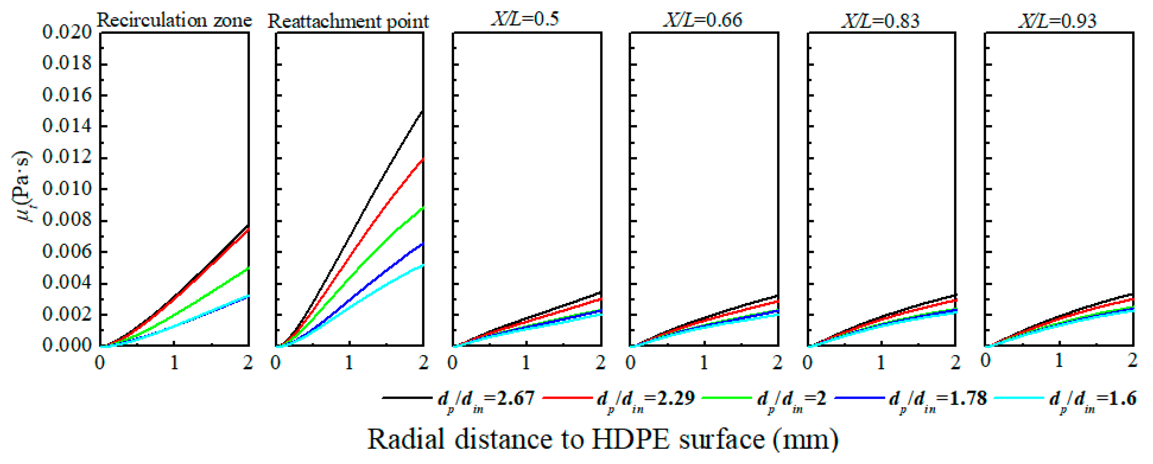
• The physical reasons for the regression rate that are affected by the sudden expansion ratio were obtained. The variation of turbulent viscosity due to the sudden expansion ratio changes could significantly affect the solid fuel regression rate and the fuel surface heat transfer.
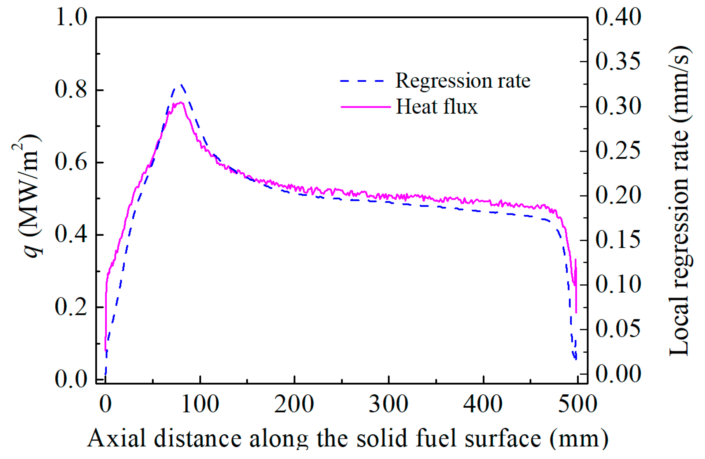
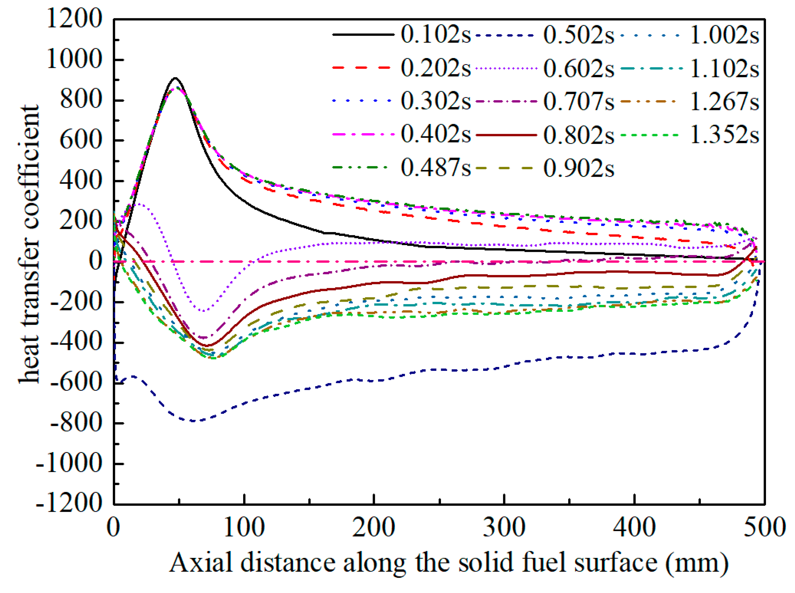
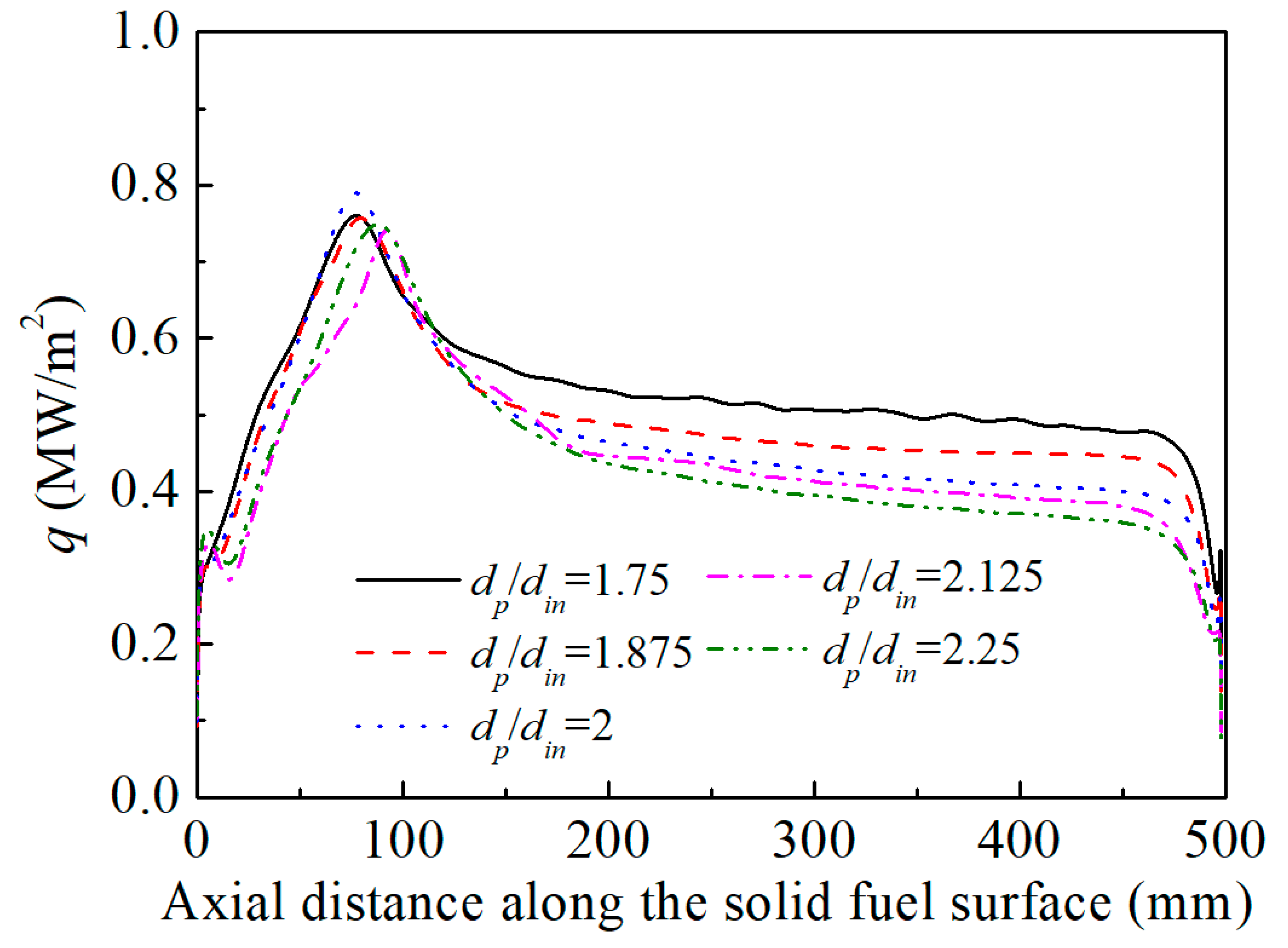
• It becomes evident that the combustion process is closely related to the heat transfer process of solid fuel surface. Based on the analysis of the heat transfer coefficient, the self-sustained combustion occurs around the reattachment point at first, and then gradually spread to the redevelopment zone. The heat released in the reattachment point will be used to achieve the self-sustained combustion in the redevelopment zone.
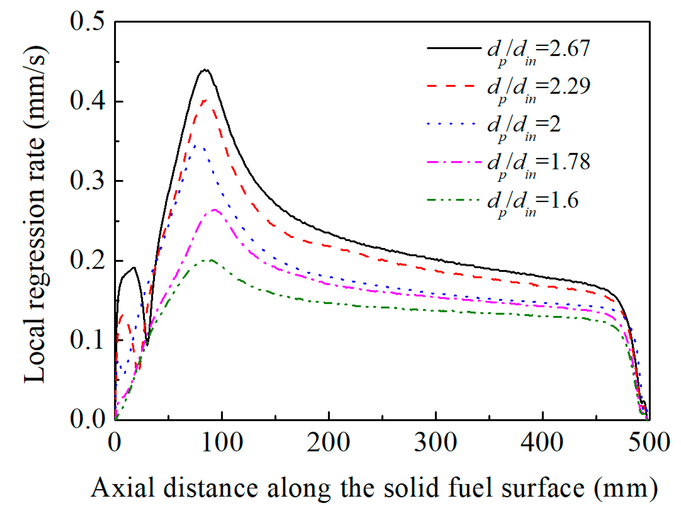
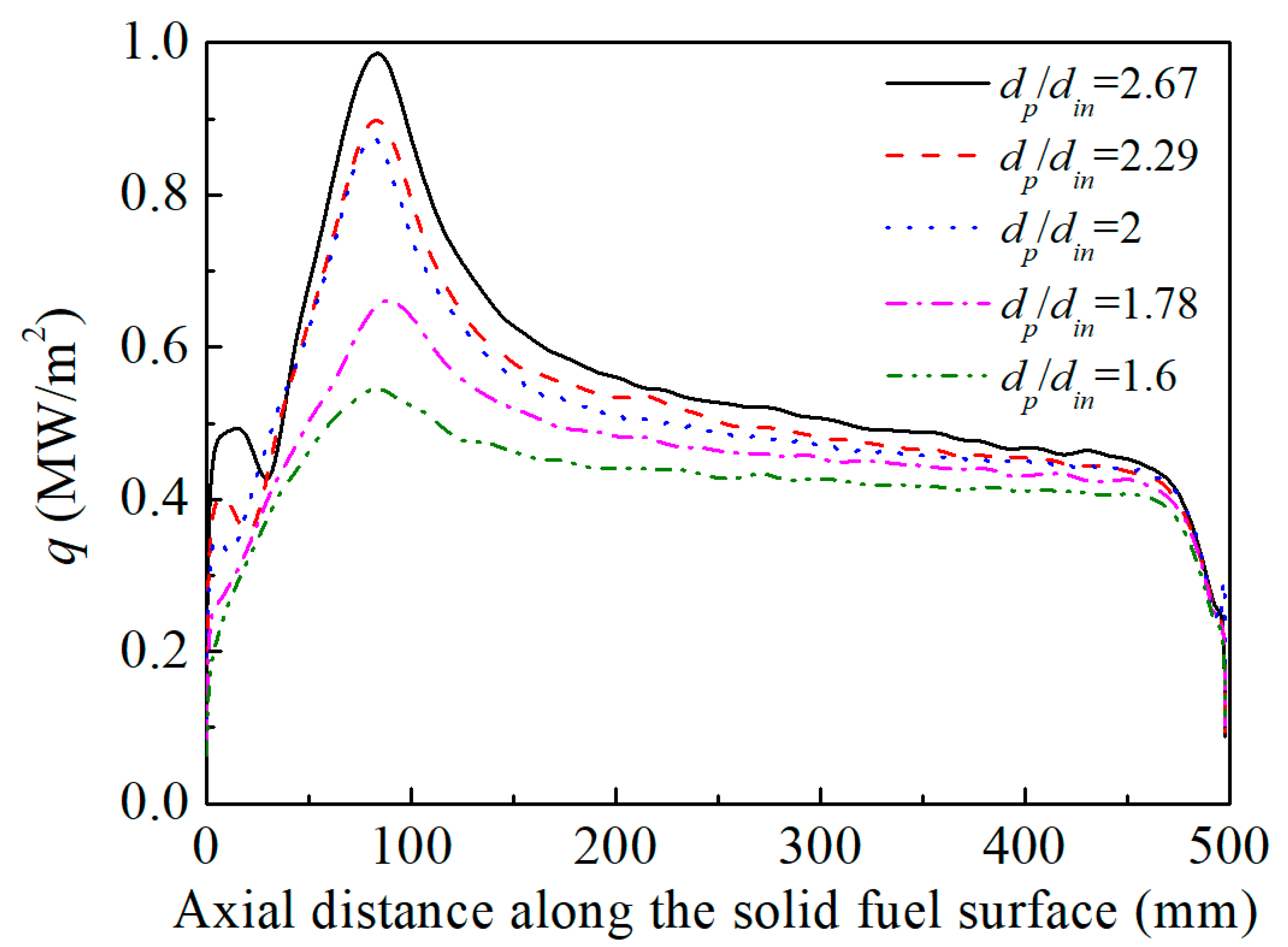
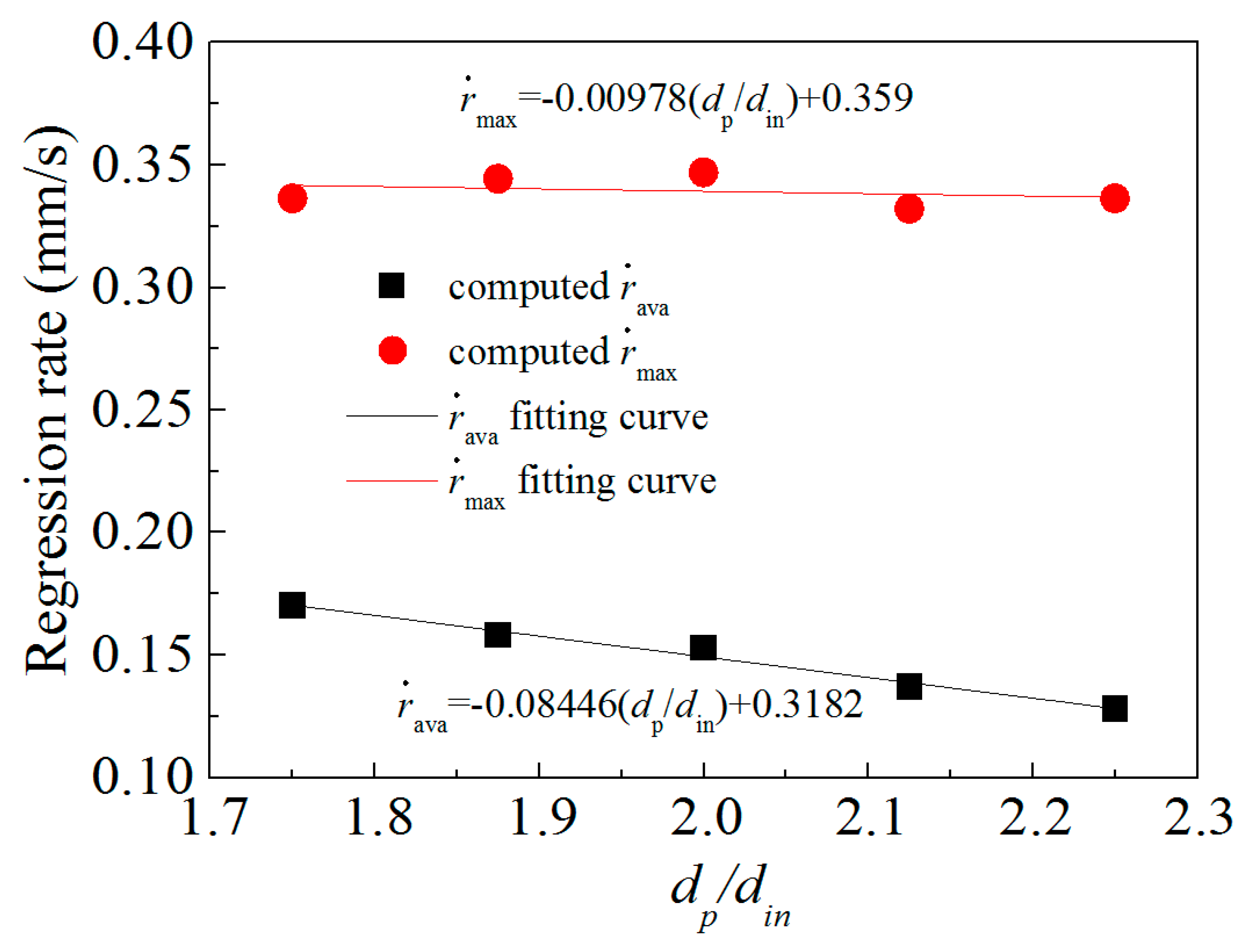
• The linear relationship between the sudden expansion ratio with fixed port diameter and average/maximum regression rate was obtained. The result indicates that the average regression rate and maximum regression rate are more sensitive to the change of the port-to-inlet diameter. Additionally, the overall heat transfer behavior of the fuel surface was mostly dominated by the maximum heat transfer around the backward-facing step.
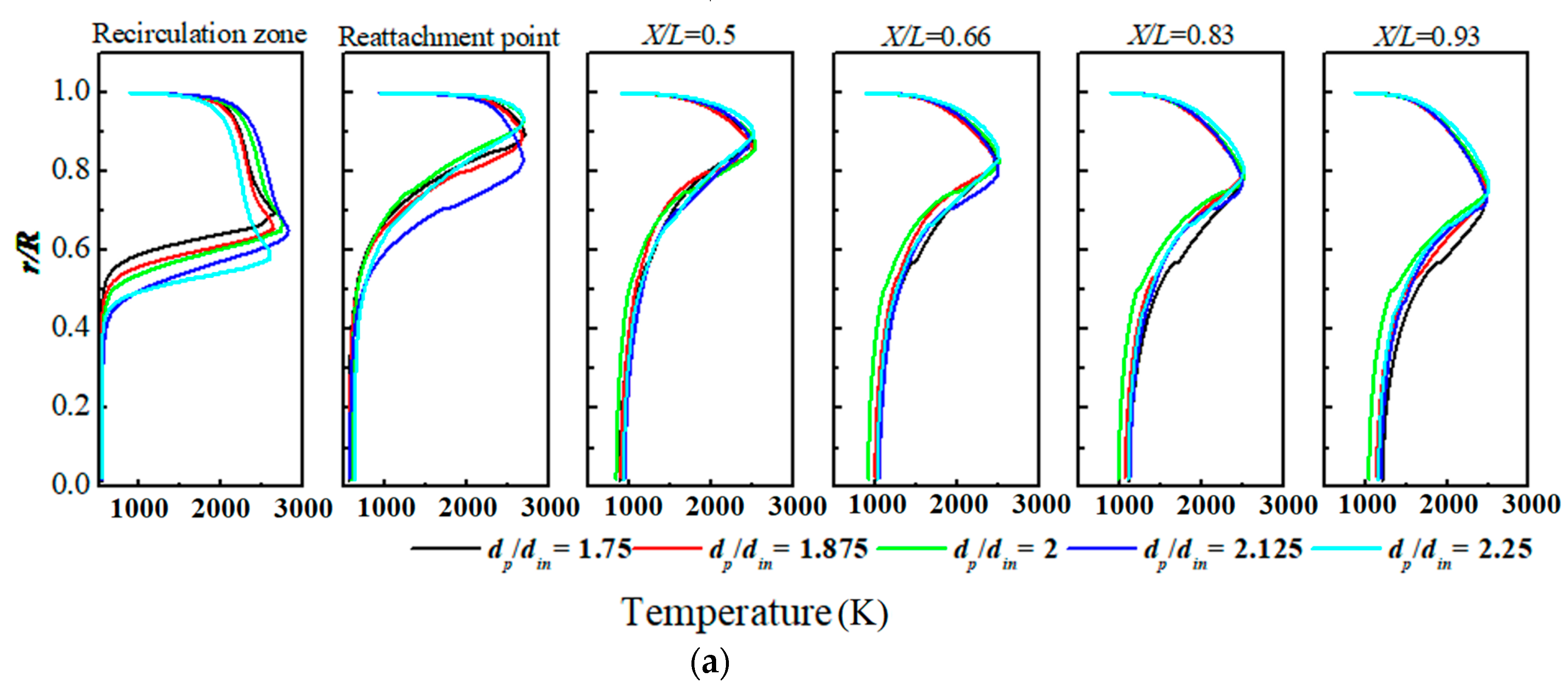
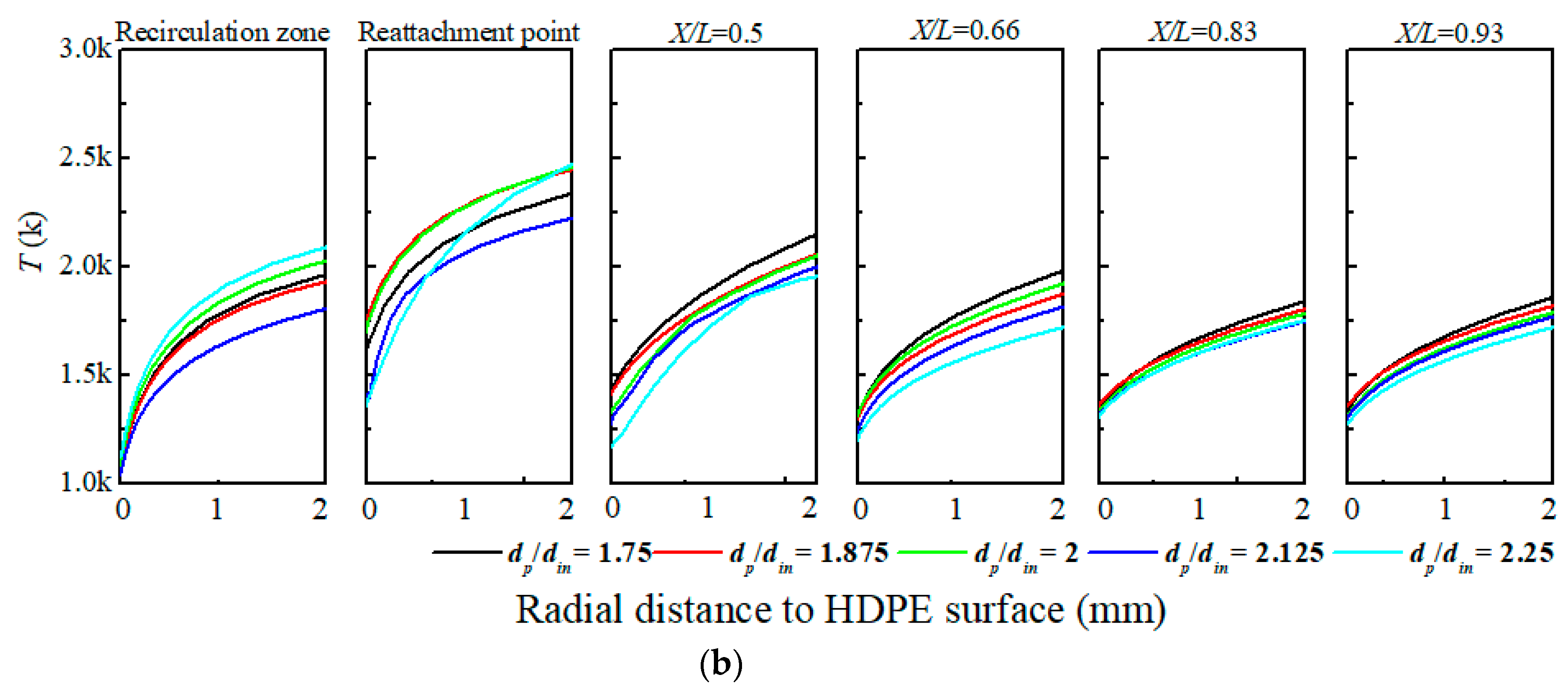
• Based on the analysis of linear relationship between regression rate and sudden expansion ratio with fixed inlet diameter. The average regression rate is mainly affected by heat transfer mechanism in a fully developed turbulent flow in rthe edevelopment zone, and it decreased with the increasing of the sudden expansion ratio.

References

1. Schulte, G. Fuel regression and flame stabilization studies of solid-fuel ramjets. J. Propuls. Power 1986, 2, 301–304. [Google Scholar] [CrossRef]
2. Gany, A.; Levy, Y.; Zvuloni, R. Geometric effects on the combustion in solid fuel ramjets. J. Propuls. Power 1989, 5, 32–37. [Google Scholar] [CrossRef]
3. Ferreira, J.; Carvalho, J., Jr.; Silva, M. Experimental investigation of polyethylene combustion in a solid fuel ramjet. In Proceedings of the 32nd Joint Propulsion Conference and Exhibit, Washington, DC, USA, 1–3 July 1996. [Google Scholar]
4. Gong, L.K.; Chen, X.; Zhou, C.S.; Li, Y. Numerical investigation on effect of solid fuel ramjet geometry on solid fuel regression rate. Acta Armament. 2016, 37, 798–807. (In Chinese) [Google Scholar]
5. Key, N.; Miller, K.L.; Fulayter, R.D. Lessons Learned from an Aggressive Outlet Vane Design for Axial Compressors. J. Propuls. Power 2012, 28, 918–926. [Google Scholar] [CrossRef]
6. Hsu, K.Y.; Carter, C.D.; Gruber, M.R.; Barhorst, T.; Smith, S. Experimental study of cavity-strut combustion in supersonic flow. J. Propuls. Power 2010, 26, 1237–1246. [Google Scholar] [CrossRef]
7. Ghodke, C.; Retaureau, G.; Choi, J.; Menon, S. Numerical and experimental studies of flame stability in a cavity stabilized hydrocarbon-fueled scramjet. In Proceedings of the AIAA International Space Planes & Hypersonic Systems & Technologies Conference, San Francisco, CA, USA, 11–14 April 2011. [Google Scholar]
8. Ghodke, C.; Choi, J.; Srinivasan, S.; Menon, S. Large eddy simulation of supersonic combustion in a cavity-strut flameholder. In Proceedings of the 49th AIAA Aerospace Sciences Meeting including the New Horizons Forum and Aerospace Exposition, Orlando, FL, USA, 4–7 January 2011. [Google Scholar]
9. Hoegl, A.; Duesterhaus, D. Measurement in a solid fuel ramjet combustion with swirl. In Proceedings of the 24th Joint Propulsion Conference, Boston, MA, USA, 11–13 July 1988. [Google Scholar]
10. Li, Y.; Li, R.; Li, D.; Bao, J.; Zhang, P. Combustion characteristics of a slotted swirl combustor: An experimental test and numerical validation. Int. Commun. Heat Mass Transf. 2015, 66, 140–147. [Google Scholar] [CrossRef]
11. Tahsini, A.M. Ignition delay time in swirling supersonic flow. Acta Astronaut. 2013, 83, 91–96. [Google Scholar] [CrossRef]
12. Jing, J.; Li, Z.; Zhu, Q.; Chen, Z.; Wang, L.; Chen, L. Influence of the outer secondary air vane angle on the gas/particle flow characteristics near the double swirl flow burner region. Energy 2011, 36, 258–267. [Google Scholar] [CrossRef]
13. Gassoumi, T.; Guedri, K.; Said, R. Numerical study of the swirl effect on a coaxial jet combustor flame including radiative heat transfer. Numer. Heat Transf. Part A Appl. 2009, 56, 897–913. [Google Scholar] [CrossRef]
14. Nemoda, S.; Bakić, V.; Oka, S.; Zivković, G.; Crnomarković, N. Experimental and numerical investigation of gaseous fuel combustion in swirl chamber. Int. Commun. Heat Mass Transf. 2005, 48, 4623–4632. [Google Scholar] [CrossRef]
15. Orbay, R.C.; Nogenmyr, K.J.; Klingmann, J.; Bai, X.S. Swirling turbulent flows in a combustion chamber with and without heat release. Fuel 2013, 104, 133–146. [Google Scholar] [CrossRef]
16. Campbell, W.H., Jr. An Experimental Investigation of the Effects of Swirling Air Flows on the Combustion Properties of a Solid Fuel Ramjet Motor; Naval Postgraduate School Monterey: Monterey, CA, USA, 1985. [Google Scholar]
17. Musa, O.; Xiong, C.; Changsheng, Z.; Li, W. Effect of inlet conditions on swirling turbulent reacting flows in a solid fuel ramjet engine. Appl. Therm. Eng. 2017, 113, 186–207. [Google Scholar] [CrossRef]
18. Musa, O.; Xiong, C.; Changsheng, Z. Experimental and numerical investigation on the ignition and combustion stability in solid fuel ramjet with swirling flow. Acta Astronaut. 2017, 137, 157–167. [Google Scholar] [CrossRef]
19. Musa, O.; Xiong, C.; Changsheng, Z.; Lunkun, G. Assessment of the modified rotation/curvature correction SST turbulence model for simulating swirling reacting unsteady flows in a solid-fuel ramjet engine. Acta Astronaut. 2016, 129, 241–252. [Google Scholar] [CrossRef]
20. Musa, O.; Xiong, C.; Chang-Sheng, Z.; Ying-Kun, L.; Wen-He, L. Investigations on the influence of swirl intensity on solid-fuel ramjet engine. Comput. Fluids 2018, 167, 82–99. [Google Scholar] [CrossRef]
21. Krishnan, S.; George, P. Solid fuel ramjet combustor design. Prog. Aerosp. Sci. 1998, 34, 219–256. [Google Scholar] [CrossRef]
22. Li, W.; Chen, X.; Musa, O.; Gong, L.; Zhu, L. Investigation of the effect of geometry of combustor on combustion characteristics of solid-fuel ramjet with swirl flow. Appl. Therm. Eng. 2018, 145, 229–244. [Google Scholar] [CrossRef]
23. Kuo, K.K. Principles of Combustion; John Wiley: Hoboken, NJ, USA, 2005. [Google Scholar]
24. Chen, J. Combustion Fundamental of Solid Rocket; Nanjing University of Science and Technology Press: Nanjing, China, 2011. (In Chinese) [Google Scholar]
25. Kee, R.J.; Rupley, F.M.; Meeks, E.; Miller, J.A. CHEMKIN-III: A FORTRAN Chemical Kinetics Package for the Analysis of Gas-Phase Chemical and Plasma Kinetics; Sandia National Labs.: Livermore, CA, USA, 1996.
26. Stoliarov, S.I.; Walters, R.N. Determination of the heats of gasification of polymers using differential scanning calorimetry. Polym. Degrad. Stab. 2008, 93, 422–427. [Google Scholar] [CrossRef]
27. Bianchi, D.; Nasuti, F.; Onofri, M. Radius of curvature effects on throat thermochemical erosion in solid rocket motors. J. Spacecr. Rockets 2014, 52, 320–330. [Google Scholar] [CrossRef]
28. Menter, F.R. Two-equation eddy-viscosity turbulence models for engineering applications. AIAA J. 1994, 32, 1598–1605. [Google Scholar] [CrossRef]
29. Vieser, W. Heat Transfer Predictions Using Advanced Two-Equation Turbulence Models; CFX Technical Memorandum (CFX-VAL10/0602); CFX: Lahore, Pakistan, 2002. [Google Scholar]
30. Kim, K.H.; Kim, C.; Rho, O.H. Methods for the accurate computations of hypersonic flows: I. AUSMPW+ scheme. J. Comput. Phys. 2001, 174, 38–80. [Google Scholar] [CrossRef]
31. Zhang, L.P.; Wang, Z.J. A block LU-SGS implicit dual time-stepping algorithm for hybrid dynamic meshes. Comput. Fluids 2004, 33, 891–916. [Google Scholar] [CrossRef]
32. Blazek, J. Computational Fluid Dynamics: Principles and Applications; Butterworth-Heinemann: Oxford, UK, 2015. [Google Scholar]
33. Musa, O.; Xiong, C.; Changsheng, Z.; Min, Z. Combustion modeling of unsteady reacting swirling flow in solid fuel ramjet. In Proceedings of the International Conference on Mechanical, Montreal, QC, Canada, 28–29 March 2017. [Google Scholar]
34. Schulte, G.; Pein, R.; Högl, A. Temperature and concentration measurements in a solid fuel ramjet combustion chamber. J. Propuls. Power 1987, 3, 114–120. [Google Scholar] [CrossRef]
35. Baurle, R.; Mathur, T.; Gruber, M.; Jackson, K. A numerical and experimental investigation of a scramjet combustor for hypersonic missile applications. In Proceedings of the 34th AIAA/ASME/SAE/ASEE Joint Propulsion Conference and Exhibit, Cleveland, OH, USA, 13–15 July 1998. [Google Scholar]
36. Chiaverini, M.J.; Harting, G.C.; Lu, Y.C.; Kuo, K.K.; Peretz, A.; Jones, H.S.; Wygle, B.S.; Arves, J.P. Pyrolysis behavior of hybrid-rocket solid fuels under rapid heating conditions. J. Propuls. Power 1999, 15, 888–895. [Google Scholar] [CrossRef]
37. Gong, L.; Chen, X.; Musa, O.; Yang, H.; Zhou, C. Numerical and experimental investigation of the effect of geometry on combustion characteristics of solid-fuel ramjet. Acta Astronaut. 2017, 141, 110–122. [Google Scholar] [CrossRef]
38. Dellenback, P.A.; Metzger, D.E.; Neitzel, G.P. Measurements in turbulent swirling flow through an abrupt axisymmetric expansion. AIAA J. 1988, 26, 669–681. [Google Scholar] [CrossRef]
39. Nejad, A.S.; Vanka, S.P.; Favaloro, S.C.; Samimy, M.; Langenfeld, C. Application of laser velocimetry for characterization of confined swirling flow. J. Eng. Gas Turbines Power 1989, 111, 36–45. [Google Scholar] [CrossRef]
40. Lehr, H.F. Experiments on shock-induced combustion. Astronaut. Acta 1972, 17, 589–597. [Google Scholar]
41. Jaojaruek, K. Mathematical model to predict temperature profile and air–fuel equivalence ratio of a downdraft gasification process. Energy Convers. Manag. 2014, 83, 223–231. [Google Scholar] [CrossRef]
Figure 1. Schematic of connected pipe test facility.
Energies 12 01784 g001
Figure 2. The experimental system.
Energies 12 01784 g002
Figure 3. Diagram of solid fuel ramjet.
Energies 12 01784 g003
Figure 4. y+ (y-axis) along the fuel surface (x-axis) of different mesh number.
Energies 12 01784 g004
Figure 5. Axial distribution of local regression rate of different mesh number.
Energies 12 01784 g005
Figure 6. Axial velocity in different axial locations for different mesh number.
Energies 12 01784 g006
Figure 7. Tangential velocity in different axial locations for different mesh number.
Energies 12 01784 g007
Figure 8. Physical model of simulation.
Energies 12 01784 g008
Figure 9. Normalized axial velocity (a) and tangential velocity (b) at different axial position.
Energies 12 01784 g009
Figure 10. The temperatures and pressures of simulation and experiment.
Energies 12 01784 g010
Figure 11. The composition distributions of simulation and experiment.
Energies 12 01784 g011
Figure 12. Temperature profiles case (a) Tw = 900 K and case (b) heat flux qw = 70 kw.
Energies 12 01784 g012
Figure 13. Internal surface of solid fuel after combustion.
Energies 12 01784 g013
Figure 14. Regression rate contour of HDPE solid fuel grain.
Energies 12 01784 g014
Figure 15. The regression rate of simulation and experiment.
Energies 12 01784 g015
Figure 16. The contour of temperature and streamline.
Energies 12 01784 g016
Figure 17. The contours of (a) mass fraction of CO2, (b) mass fraction of CO, and (c) mass fraction of O2.
Energies 12 01784 g017
Figure 18. Radial profiles of axial (a) and tangential velocity (b) at different axial positions along the combustor.
Energies 12 01784 g018
Figure 19. Temperature at different axial positions in the combustor.
Energies 12 01784 g019
Figure 20. The local regression rate of different time.
Energies 12 01784 g020
Figure 21. The profiles of local heat flux and regression rate along the solid surface.
Energies 12 01784 g021
Figure 22. Radial profi1es of temperature (a), turbulent viscosity (μt) (b) at different axial positions.
Energies 12 01784 g022
Figure 23. The heat transfer coefficient along high-density Polyethylene (HDPE) surface of different time for swirl flow.
Energies 12 01784 g023
Figure 24. Local regression rate obtained from simulation for different cases.
Energies 12 01784 g024
Figure 25. The local heat flux for different cases.
Energies 12 01784 g025
Figure 26. Temperature (a) and temperature around fuel surface (b) at different axial positions of different cases.
Energies 12 01784 g026
Figure 27. Turbulent viscosity (μt) at different axial positions of different cases.
Energies 12 01784 g027
Figure 28. Local regression rate obtained from simulation for different cases.
Energies 12 01784 g028
Figure 29. The local heat flux along the solid surface.
Energies 12 01784 g029
Figure 30. Temperature (a) and temperature around HDPE grain surface (b) at different axial positions of different cases.
Energies 12 01784 g030aEnergies 12 01784 g030b
Figure 31. Radial profiles of the turbulent viscosity (μt) at different axial positions in, solid fuel ramjet (SFRJ) combustor of different cases.
Energies 12 01784 g031
Figure 32. Regression rate for different sudden expansion ratio with dp fixed as constant.
Energies 12 01784 g032
Figure 33. The regression rate for different sudden expansion ratio with din fixed as constant.
Energies 12 01784 g033
Figure 34. The regression rate for different sudden expansion ratio with dp fixed as constant.
Energies 12 01784 g034
Figure 35. The regression rate for different sudden expansion ratio with din fixed as constant.
Energies 12 01784 g035