Article

Comparative Analysis of Different Methodologies Used to Estimate the Ground Thermal Conductivity in Low Enthalpy Geothermal Systems

by
Cristina Sáez Blázquez
*,
Ignacio Martín Nieto
,
Arturo Farfán Martín
,
Diego González-Aguilera
and
Pedro Carrasco García
Department of Cartographic and Land Engineering, University of Salamanca, Higher Polytechnic School of Avila, Hornos Caleros 50, 05003 Avila, Spain
*
Author to whom correspondence should be addressed.
Energies 2019, 12(9), 1672; https://doi.org/10.3390/en12091672
Submission received: 3 April 2019 / Revised: 25 April 2019 / Accepted: 29 April 2019 / Published: 2 May 2019
(This article belongs to the Special Issue Volume II: Low Enthalpy Geothermal Energy)

Abstract

:
In ground source heat pump systems, the thermal properties of the ground, where the well field is planned to be located, are essential for proper geothermal design. In this regard, estimation of ground thermal conductivity has been carried out by the implementation of different techniques and laboratory tests. In this study, several methods to obtain the thermal properties of the ground are applied in order to compare them with the reference thermal response test (TRT). These methods (included in previous research works) are carried out in the same geological environment and on the same borehole, in order to make an accurate comparison. All of them provide a certain value for the thermal conductivity of the borehole. These results are compared to the one obtained from the TRT carried out in the same borehole. The conclusions of this research allow the validation of alternative solutions based on the use of a thermal conductive equipment and the application of geophysics techniques. Seismic prospecting has been proven as a highly recommendable indicator of the thermal conductivity of a borehole column, obtaining rate errors of below 1.5%.

1. Introduction

The global growing energy needs have sparked renewed interest in ground source heat pump systems. These systems are traditionally used for space heating and cooling by the extraction of the ground’s energy through a borehole heat exchanger (BHE) [1]. High initial investments are commonly associated with these installations so that an optimal ground loop dimensioning is advisable to avoid unnecessary costs. In this regard, the design process requires knowing rather accurately the thermal conductivity of geological formation where the ground source heat pump (GSHP) system will be located [2,3]. Ground thermal conductivity is usually determined by the implementation of a Thermal Response Test (TRT), the main purpose of which is the measuring of the equivalent thermal conductivity of the ground volume tested and the thermal resistance of the BHE [4,5,6,7]. The conventional TRT is based on circulating heated water in a closed loop, which simulates heat transfer occurring in a ground heat exchanger. Inlet and outlet water temperatures and flow rate are measured during the test. These data are then analyzed by the implementation of analytical or numerical models that allow determining the ground thermal conductivity and the borehole thermal resistance [8,9]. The most used interpretation technique relies on the first-order approximation of the infinite line-source model. Assuming a constant heating power, a linear regression model is fitted to the late temperature measurements to calculate the mean time derivative of the temperature and deduct the desired parameters. This first approach to linearize the infinite line source model requires rejecting the early measurements for the subsequent test interpretation. TRT duration is usually established between 36‒72 h, but this duration has been thoroughly discussed in the past [10] and at the moment is an area of active research [11,12,13,14,15]. Despite the errors these test could involve [4], the high accuracy of ground thermal conductivity results represent essential information in the corresponding geothermal loop sizing. The main inconvenience associated with the realization of a TRT is its relatively high cost (around 3000 Euros), remaining an issue that prevents its widespread use. This problem is especially significant in small installations, where the test increases the initial investment without clear compensation.
Focusing on alternative solutions, some variations of a TRT are available in the existing literature. For example, Henke et al. [16] proposed an experimental apparatus that, as a TRT, measures the temperature response of a borehole. Freifeld et al. [17] developed a borehole methodology to estimate the formation thermal conductivity in situ with spatial resolution of one meter. However, the alternative techniques found in other authors’ researches have similar economic issues [18] and their validity is still unclear.
In this research, a series of methodologies (already published and available in the current literature), aimed at the estimation of the ground thermal conductivity, are applied on a real area. These techniques are then evaluated by their comparison with the results of a thermal response test carried out on a borehole placed in the same location. In a nutshell, the thermal conductivity of a certain geological environment is determined by the implementation of affordable methods whose validity is thoroughly assessed. Thus, the main problematic addressed in this work is characterization of ground thermal from different methods to generally improve the design of a low enthalpy geothermal system.

2. Materials and Methods

2.1. Global Description of the Area under Study

The comparison of the methodologies considered in this research is derived from the thermal characterization of a 43 m length and 220 mm diameter borehole placed in the province of Ávila (Spain). The exact location of this well is detailed in Table 1.
The area contemplated in the present research is located in the center of Ávila (Spain). This region is geologically constituted by two main blocks. One of them is defined by igneous and metamorphic rocks from the Upper Carboniferous-Low Permian and Pre-Cambrian-Low Cambrian periods, respectively. The second block is characterized by the presence of sedimentary materials from the Mesozoic, Tertiary and Quaternary (oriental area of the Amble’s valley) periods [19,20]. In the case of the volume of ground considered here, it belongs to granite formations and more specifically, adamellite rocks. This information can be deduced from the geological map of the region presented in Figure 1.
For a more precise geological characterization, geophysical tests were applied on the experimental borehole. A well logging system was used to obtain the specific earth information. It consists of the measuring of continuous and simultaneous record of different physical parameters throughout the borehole column. The equipment used for the mentioned purpose utilizes a series of interchangeable multi-parameter sensors that allowed to register the following parameters: spontaneous potential, resistivity, and natural gamma radiation. Figure 2 includes the register of the well logging test applied on the study borehole and the stratigraphic column derived from its interpretation.
Once the geological levels that constitute the ground in the area of the borehole were accurately defined, different tests were conducted in the area with the objective of determining the thermal conductivity of the materials previously detected. The implemented methodologies are described in the following subsections.

2.2. Thermal Conductivity Characterization

The principal purpose of this section is the estimation of the thermal conductivity of the borehole column described above. To that end, different methods and procedures implemented in previous author’s researches are considered here to finally compare them with the results of a TRT. The following subsections contain the description of each of the mentioned thermal conductivity estimator techniques.

2.2.1. KD2 Pro Measurements

In a previous research work, the thermal conductivity map of the province of Ávila (study area of this research) was created from experimental measurements on the principal geological formations of the region. Representative rocky samples were collected and taken to the laboratory, where the thermal conductivity parameter was measured.
After systematic sample processing—drilling and carving obtaining samples with a specific size, removal of excess material—KD2 Pro equipment was used to measure the thermal conductivity of each geological formation. Before its use, a hole of 6 cm length and 3.9 mm in diameter was made on each rocky sample in order to introduce the RK-1 sensor of KD2 Pro device. More information about the specific measuring methodology is provided in the full published version of the manuscript [21].
As a result of the KD2 Pro measurement, the mentioned research provides the thermal conductivity of the rocky and soil formations. According to the borehole column in Figure 2, the volume of ground under study is constituted by different layers of materials. In order to obtain a representative thermal conductivity value of the whole column well, the thermal conductivity of each layer and its thickness must be considered. Based on the results offered in the research, thermal conductivities of the borehole materials were deduced. All this information is included in Table 2. Thermal conductivity values presented in Table 2 correspond to the average values registered for each geological formation in the manuscript considered here. However, for the last layer of altered adamellites, the lowest values of the mentioned study were selected due to the presence of loose materials and the altered state of granite rocks in that level.
Finally, the thermal conductivity representative of the whole studied borehole can be obtained from the application of Equation (1) and the information previously attached in Table 2.
k T ( W / mK ) = k 1 · T 1 + k 2 · T 2 + k 3 · T 3 + k 4 · T 4
where:
  • kT = Global thermal conductivity of the whole borehole column.
  • k1 = Thermal conductivity of the geological formation of layer 1.
  • k2 = Thermal conductivity of the geological formation of layer 2.
  • k3 = Thermal conductivity of the geological formation of layer 3.
  • k4 = Thermal conductivity of the geological formation of layer 4.
  • T1 = Thickness of layer 1 expressed as a percentage of the total well thickness.
  • T2 = Thickness of layer 2 expressed as a percentage of the total well thickness.
  • T3 = Thickness of layer 3 expressed as a percentage of the total well thickness.
  • T4 = Thickness of layer 4 expressed as a percentage of the total well thickness.

2.2.2. Geophysics

Geophysical prospecting has been used in previous works as a ground thermal conductivity estimator. The principal basis of these studies is the correlation of a geophysical parameter and thermal conductivity measurements (using KD2 Pro device) to finally predict the thermal behavior of the ground in depth. A more detailed description of these methods and their implementation in the area of the present research is included in the following subsections.
(1) Seismic data:
The first geophysical method makes reference to the implementation of seismic prospecting tests. In a previous research work, the mentioned tests were implemented on three different geological formations (schists, medium grain and coarse-grained adamellites) using MASW and seismic refraction techniques in order to register P and S waves velocities. At the same time, thermal conductivity of each formation was measured by the use of KD2 Pro equipment. These tests were made on the most and least decomposed samples of each geological environment to find the lowest and highest conductivity values. Finally, this published research correlates the propagation velocities of P and S waves and the thermal conductivity of samples from the same material [22].
The ultimate result of this work is to predict the thermal behavior of the geological formations included in the study. By identifying the propagation velocities of the seismic waves in a certain area, the evolution of the thermal conductivity of the ground in that area can be evaluated. Thus, 2D thermal conductivity sections provided in the mentioned research allow estimation of the evolution of ground thermal conductivity in depth for each specific formation.
In order to ensure application of this methodology, seismic refraction tests were conducted on the area where the borehole of study is located. The results of these tests are provided in Figure 3.
After the distribution of the P wave velocity was identified in depth, different thermal conductivity measurements were taken in order to identify the most and least thermal conductive samples, meaning those with the highest and lowest compaction levels. These values correspond to the minimum thermal conductivity of anthropogenic fills and the maximum thermal conductivity for the altered adamellite; they are presented in Table 3. It should be noted that altered adamellites were extracted from the drilling process at depths where they were identified. These samples were then used in thermal conductivity characterization.
By measuring P wave velocity and thermal conductivities in the study area, the correlation between both parameters was obtained (graphically presented in Figure 4). This is based on pairing the lowest thermal conductivity value with the lowest p wave velocity (in the same area) and the highest thermal conductivity with the highest p wave velocity. More information on this method is provided in the mentioned published research.
From the above correlation and by following the instructions of the mentioned research, the distribution of the thermal conductivity parameter in the area considered here is displayed in the 2D section of Figure 5.
According to Figure 5, the volume of ground included under the borehole is constituted by a set of layers with different thermal conductivity values. This information can be observed in Table 4.
Finally, the global thermal conductivity of the borehole column is deduced from the application of the above data (Table 4) in Equation (1).
(2) Electrical resistivity:
In this case, electrical resistivity data were collected to finally create a 3D thermal conductivity map of the area of interest. The fundamentals of this method are similar to the one explained before; electrical resistivity results are correlated with thermal conductivity measurements and a relation between both parameters is obtained for a certain geological formation. The research work, including this methodology, was focused on granite rocks (adamellites), and the electrical resistivity was obtained using the Electrical Resistivity Tomography (ERT) technique. Thermal conductivity measurements were, in turn, taken using KD2 Pro equipment following the same operational procedure (tests were made on the most and least decomposed rocky samples) [23].
The results of this research disclose a certain relation between thermal conductivity and electrical resistivity. This relation can be observed in Equation (2).
k =   2 · 10 7 x 2 + 0.0001 x + 1.4881
where:
  • k = thermal conductivity (W/mK)
  • x = electrical resistivity (Ω·m)
To apply Equation (2), the electrical resistivity of the materials in the study area must be known. To this end, an ERT test was conducted around the mentioned area, obtaining a 2D electrical resistivity section (presented in Figure 6).
On interpretation of the above 2D electrical resistivity section, the borehole considered in this study is constituted by a series of layers with different thickness and characterized by variable electrical resistivity values. All these data are included in Table 5; the thermal conductivity of each layer is obtained by application of Equation (2).
As in the previous cases, Equation (1). must be used to finally define the global thermal conductivity of the borehole column from partial thermal conductivity values and thickness of each layer.

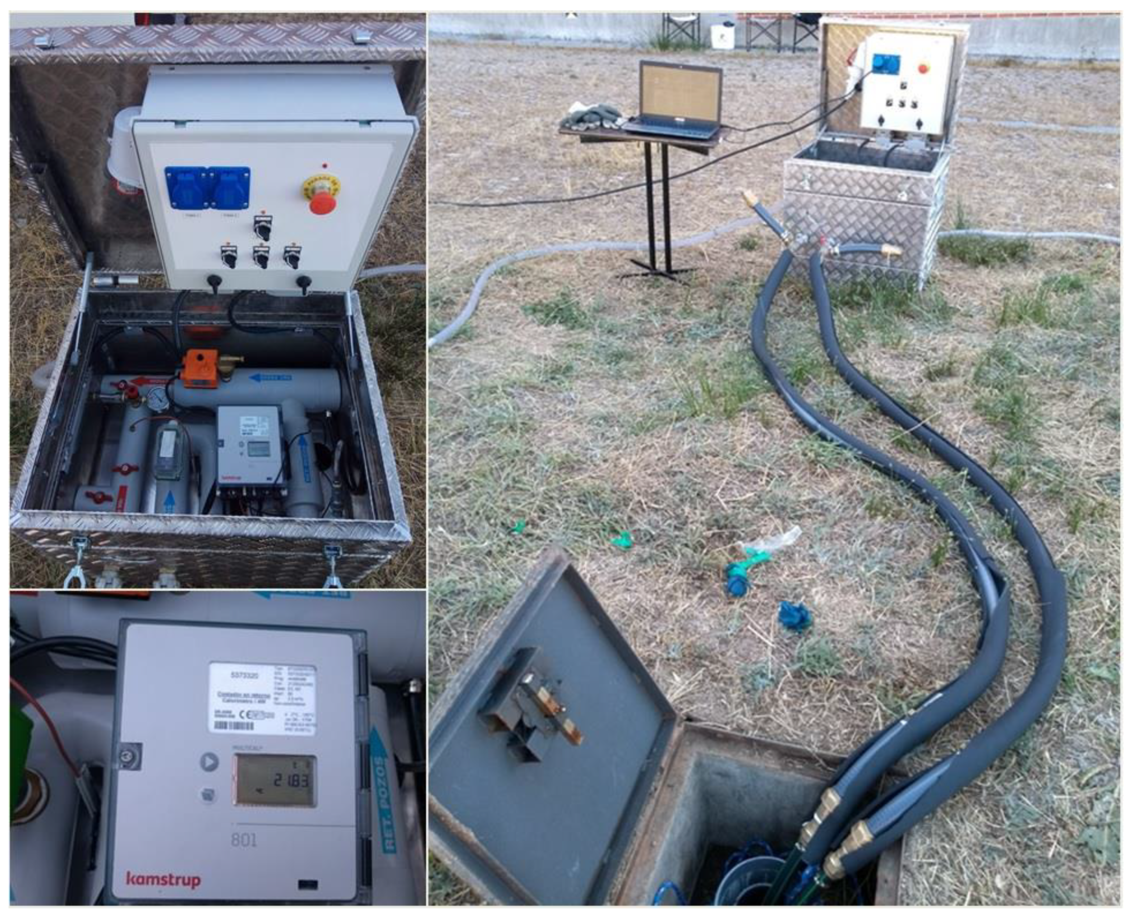
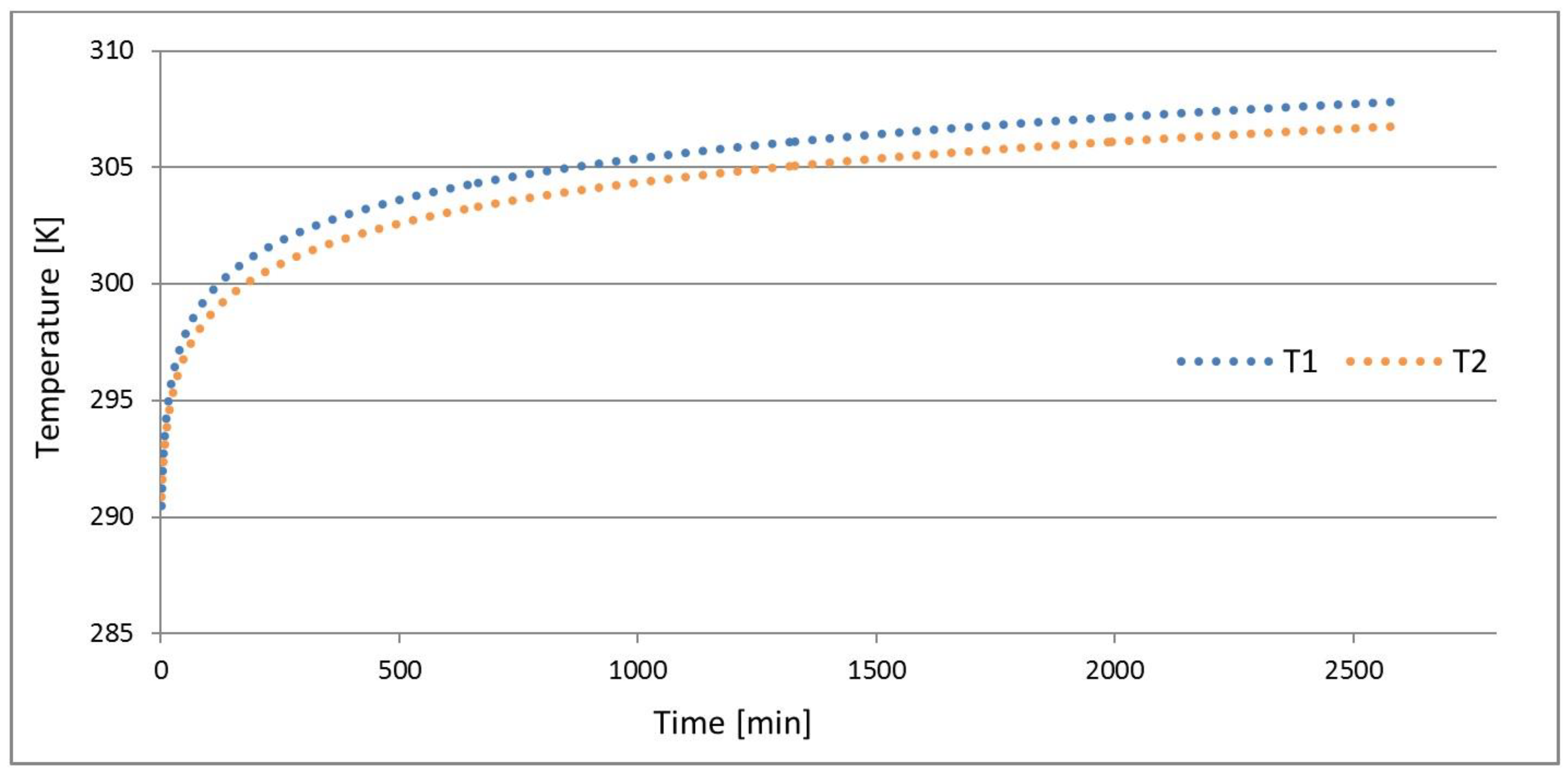
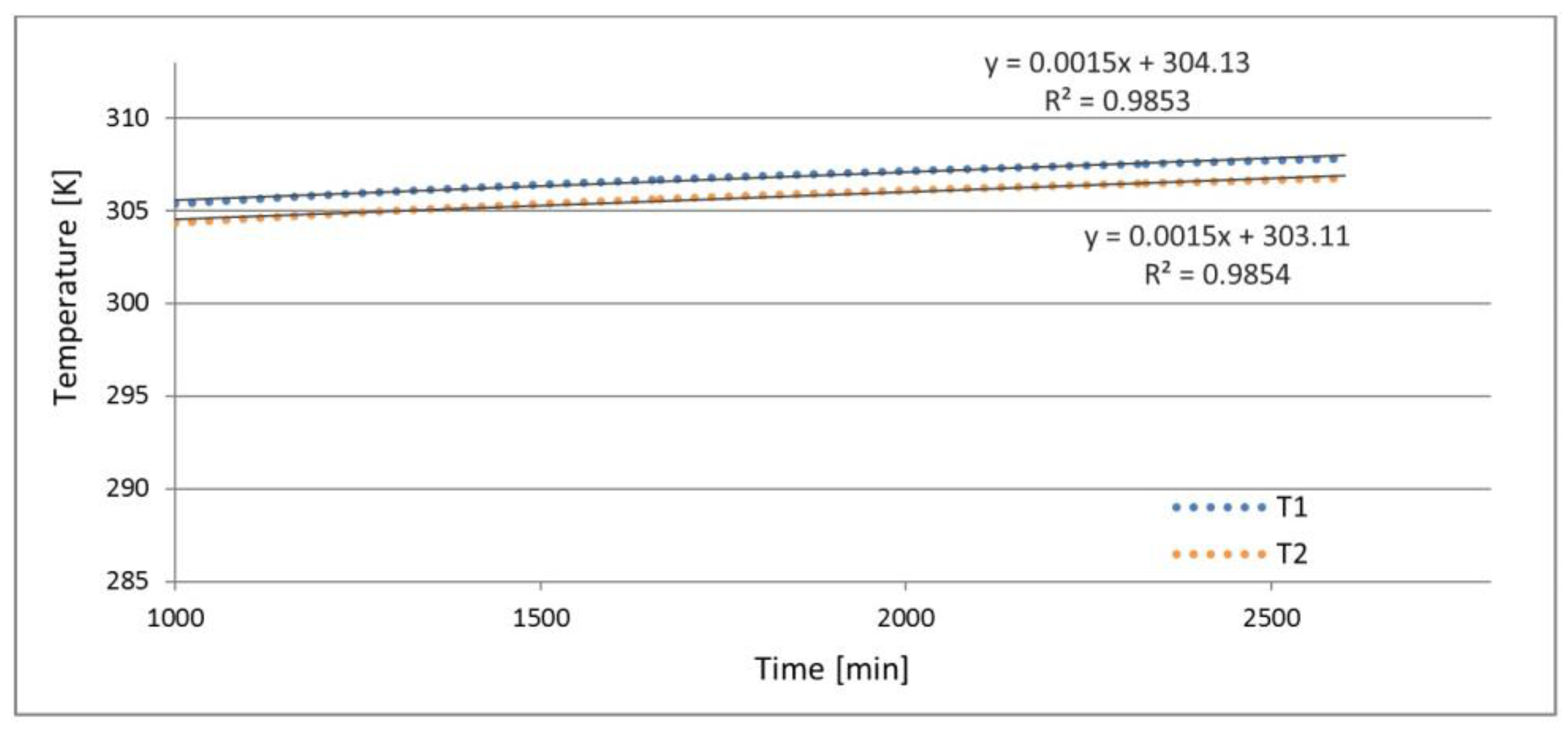
2.2.3. Thermal Response Test

The last procedure implemented in this research is the realization of a Thermal Response Test in the borehole. These tests are routinely used to estimate borehole thermal properties with regard to the mentioned thermal conductivity. The conventional TRT consists of circulating heated fluid (usually water) in a closed loop. During the test, fluid temperatures are measured at the ground heat exchanger inlet and outlet, along with the flow rate. Theses measured values are then analyzed by analytical or numerical models with the aim of calculating thermal conductivity and borehole thermal resistance [3,24].
(1) Test implementation
First, the borehole was geothermally prepared for the test by installing a polyethylene single-U tube heat exchanger of 32 mm with spacers located one meter apart. Taking advantage of the high groundwater level in the area, grouting material was not used [25,26]. The working fluid was water (during the test, low ambient temperatures were not expected) and the connection of the inlet and outlet heat exchangers and the TRT device was made with polyethylene tubes that were externally insulated. In order to set the initial condition of this test, a temperature register (PCE-T recorder) was used to measure the base temperature of the ground, obtaining a constant value of 14.6 °C at a depth of 40 m.
In this research, TRT was done according to UNE-EN ISO 17628:2017 regulations [27]. The TRT device implemented here constituted of a heat injection system, a circulating pump, and electrical resistance as heat source. The resistance allows three different heating levels, corresponding to the injection of 3 kW (stage 1), 6 kW (stage 2), and 9 kW (stage 3). The TRT equipment also included a Kamstrup energy meter (to register a large number of parameters), commercially known as MULTICAL 801.
Once the borehole was properly equipped, the sequence of events was as follows:
-
Circuit filling and establishment of the appropriate working pressure.
-
Activation of the circulating TRT pump and starting of the first heating stage (3 kW).
-
General system operation during a certain period of time.
-
Downloading and data management from the Kamstrup register.
-
Calculation of the global thermal conductivity parameter.
The TRT duration is a controversial subject—while reducing TRT duration could help reduce costs, the accuracy of results could be affected. Following the regulation mentioned before [27], the minimum duration of the TRT can be estimated by Equation (3).
t   ( s ) =   5 · r 2 α
where:
  • r = borehole radius (m)
    α = k e c v
  • ke = estimated thermal conductivity (W/mK)
  • cv = volumetric thermal capacity (J/m3/K)
By applying Equation (3) and estimating thermal conductivity of 1.80 W/mK and volumetric thermal capacity of 2.16 × 10⁶ J/m3/K [28], the minimum duration required for the thermal response test in the studied borehole would be:
t   ( s ) = 5 · 0.11 2 8.3 · 10 7 = 72891.   56   s     20.25   h
Despite this value, the real duration of the test was 43 h, which sought to guarantee total stabilization of the system. Additionally, Figure 7 shows the TRT device and some sequences of the test.
(2) Thermal conductivity calculation
In a borehole heat exchanger of sufficient length in comparison with its radius, the analytical solution of Kelvin’s Line Source can be applied to solve the heat equation and analyze TRT data. According to the infinite line-source model (use as a laboratory method since 1905), the thermal conductivity parameter can be obtained from the constant power rate and the slope of the temperature variation in time [29,30]. The interpretation of TRT results relies on a first-order approximation to linearize the mentioned infinite line-source model, neglecting the early measurements.
k =   Q b · 4 · π · H
where:
  • Q = heat flux (kW/min)
  • b = slope (min)
  • H = borehole length (m)

3. Results and Discussion

3.1. Previous Methods Results

Thermal conductivity results of each method considered in this research are shown in Table 6. These results are obtained by the application of the stages described for each individual procedure. The methodologies belong to validated and already published researches. Consequently, the validity of the mentioned results is guaranteed.

3.2. TRT Results

In addition to the thermal conductivity results deduced from the alternative methodologies, the TRT also provided a thermal conductivity value that will be compared with the ones in Table 6. After the corresponding operation of the TRT during the established period of time (43 h), inlet (T1) and outlet (T2) temperatures were registered (shown in Figure 8). It should be mentioned that the low temperature difference between T1 and T2 (displayed in Figure 8) is derived from the fact that the borehole length is only 43 m.
From these results, the linear approximation required for the calculation of the thermal conductivity parameter was made for the period of time up to 1000 min (discarding the early measurements) in each temperature register. Figure 9 presents the equation of each linear approximation, consequently using the slope of these lines in corresponding thermal conductivity calculations. As shown in Figure 9, the interpretation of the TRT and the subsequent calculation of the thermal conductivity parameter is made by measuring the inlet and outlet fluid temperatures for time up to 1000 min.
On observing Figure 9, we note that the slope of the linear approximation is the same for T1 and T2, such that the calculation of the thermal conductivity parameter is identical for both cases. When applying Equation (4), the following values were considered: b = 0.0015 min, H = 43 m and Q = 1.875 kW/min (resistance first stage (3000 kW)/time of the linear approximation (1600 min)). Thus, the global thermal conductivity of the borehole from TRT results takes a value of 2.313 W/mK.

3.3. General Comparison

Figure 10 graphically displays the results of each methodology considered in this research. It shows strong agreement in results between the different methods.
It is thus convenient to include the accuracy error of each of the methodologies shown in Figure 10: 10% for KD2 Pro, 14.2% for seismic prospecting, 16.7% for electrical resistivity, and 5% for TRT [4,31,32,33].
Considering TRT thermal conductivity value as the most accurate one and taking into account Figure 10, the following statements can be made:
  • Thermal conductivities obtained by the alternative techniques are in strong agreement with the TRT result. The seismic prospecting method provides the most similar value, with a difference of only 0.024 W/mK with respect to the TRT value.
  • The use of electrical resistivity tomography also allows to obtain thermal conductivity values close to the TRT result. In this case, the difference between both methods is 0.316 W/mK.
  • The least accurate method is the use of the thermal conductivity map obtained by in situ KD2 Pro measurements. Despite having the least accuracy of all the procedures considered here, the difference with respect to the TRT is 0.358 W/mK.
  • By evaluating the mentioned differences in terms of percentage, the errors of each alternative methodology in comparison with the TRT are 15.48% for the thermal conductivity map, 1.04% for seismic prospecting, and 13.66% when applying electrical resistivity tomography.

4. Conclusions

TRT has been traditionally considered an appropriate technique to provide accurate thermal conductivity values of a borehole column. However, the high costs of these tests usually prompt researchers to look for alternative solutions that help characterize ground thermal behavior. This research integrates different existing methodologies to evaluate their validity through the results of a TRT made on the same study area. Provided that TRT is not always viable and based on the final results of this work, the most recommendable technique to be applied is seismic prospecting. It has been proved that this procedure is capable of providing highly accurate thermal conductivity values with errors below 1.5%. The high ground water level of the area may be a cause of deviation from the electrical and KD2 Pro methods, due to their sensitivity to this factor.
The remaining methodologies evaluated in this research could also be appropriate solutions to obtain approximate ground thermal conductivity. In the absence of a TRT or seismic profiles, the thermal conductivity map or electrical resistivity tomography could be of great help in ground thermal conductivity characterization. Despite the obvious advantages of TRT, the deep local nature of this test could be mitigated by using geophysical methods, as the ones presented in this study. The estimation of this parameter will be incredibly useful for the corresponding geothermal design, adjusting the number of boreholes and the total drilling length required in the shallow geothermal system. In view of the importance of identifying ground thermal conductivity in a GSHP system, the conclusions of this work are highly significant in the geothermal field.

Author Contributions

All authors performed the experimental and theoretical basis of the research. C.S.B., A.F.M. and I.M.N. implemented the methodology and calculations and analyzed the results. D.G.-A. provided technical and theoretical support. P.C.G. carried out the geophysics tests. C.S.B. wrote the manuscript and all authors read and approved the final version.

Funding

This research received no external funding.

Acknowledgments

The authors would like to thank the Department of Cartographic and Land Engineering of the Higher Polytechnic School of Avila, University of Salamanca, for allowing us to use their facilities and their collaboration during the experimental phase of this research. The authors also want to thank the Ministry of Education, Culture and Sport for providing a FPU Grant (Training of University Teachers Grant) to the corresponding author of this paper, making possible the realization of this work.

Conflicts of Interest

The authors declare no conflict of interest.

References

  1. Ally, M.R.; Munk, J.D.; Baxter, V.D.; Gehl, A.C. Exergy analysis of a two-stage ground source heat pump with a vertical bore for residential space conditioning under simulated occupancy. Appl. Energy 2015, 155, 502–514. [Google Scholar] [CrossRef] [Green Version]
  2. Han, C.; Yu, X.B. Performance of a residential ground source heat pump system in sedimentary rock formation. Appl. Energy 2016, 164, 89–98. [Google Scholar] [CrossRef] [Green Version]
  3. Pasquier, P. Interpretation of the first hours of a thermal response test using the time derivative of the temperature. Appl. Energy 2018, 213, 56–75. [Google Scholar] [CrossRef]
  4. Henk, J.L. Witte, Error analysis of thermal response tests. Appl. Energy 2013, 109, 302–311. [Google Scholar]
  5. Pasquier, P.; Zarrella, A.; Marcotte, D. A multi-objetive optimization strategy to reduce correlation and uncertainty for thermal response test analysis. Geothermics 2019, 79, 176–187. [Google Scholar] [CrossRef]
  6. Bandos, T.V.; Montero, Á.; Fernández de Córdoba, P.; Urchueguía, J.F. Improving parameter estimates obtained from termal response tests: Effect of ambient air temperature variations. Geothermics 2011, 40, 136–143. [Google Scholar] [CrossRef]
  7. Choi, W.; Ooka, R. Interpretation of disturbed data in thermal response tests using the infinite line source model and numerical parameter estimation method. Appl. Energy 2015, 148, 476–488. [Google Scholar] [CrossRef]
  8. ASHRAE. Geothermal energy. In ASHRAE Handbook Heating, Ventilating, and Air-Conditioning Applications; American Society of Heating, Refrigerating and Air-Conditioning Engineers: Atlanta, GA, USA, 2007; pp. 32.1–32.30. [Google Scholar]
  9. Gehlin, S.; Hellström, G. Comparison of four models for thermal response test evaluation. ASHRAE Trans. 2003, 109, 131–142. [Google Scholar]
  10. Spitler, J.D.; Gehlin, S.E. Thermal response testing for ground source heat pump systems: An historical review. Renew. Sustain. Energy Rev. 2015, 50, 1125–1137. [Google Scholar] [CrossRef]
  11. Beier, R.A.; Smith, M.D. Minimum duration of in-situ tests on vertical boreholes. ASHRAE Trans. 2003, 109, 475–486. [Google Scholar]
  12. Bozzoli, F.; Pagliarini, G.; Rainieri, S.; Schiavi, L. Short-time thermal response test based on a 3-D numerical model. J. Phys. Conf. Ser. 2012, 395, 012–056. [Google Scholar] [CrossRef]
  13. Bujok, P.; Grycz, D.; Klempa, M.; Kunz, A.; Porzer, M.; Pytlik, A.; Rozehnal, Z.; Vojčinák, P. Assessment of the influence of shortening the duration of TRT (thermal response test) on the precision of measured values. Energy 2014, 64, 120–129. [Google Scholar] [CrossRef] [Green Version]
  14. Poulsen, S.; Alberdi-Pagola, M. Interpretation of ongoing thermal response tests of vertical (BHE) borehole heat exchangers with predictive uncertainty based stopping criterion. Energy 2015, 88, 157–167. [Google Scholar] [CrossRef]
  15. Choi, W.; Kikumoto, H.; Choudhary, R.; Ooka, R. Bayesian inference for thermal response test parameter estimation and uncertainty assessment. Appl. Energy 2018, 209, 306–321. [Google Scholar] [CrossRef]
  16. Witte, H.J.L.; van Gelder, G.J.; Spitler, J.D. In Situ Measurement of Ground Thermal Conductivity: The Dutch Perspective. ASHRAE Trans. 2002, 108, 859–867. [Google Scholar]
  17. Freifeld, B.M.; Finsterle, S.; Onstott, T.C.; Toole, P.; Pratt, L.M. Ground surface temperature reconstructions: Using in situ estimates for thermal conductivity acquired with a fiber optic distributed thermal perturbation sensor. Geophys. Res. Lett. 2008, 35, L14309. [Google Scholar] [CrossRef]
  18. Sharqawy, M.H.; Said, S.A.; Mokheimer, E.M.; Habib, M.A.; Badr, H.M.; Al-Shayea, N.A. First in situ determination of the ground thermal conductivity for borehole heat exchanger applications in Saudi Arabia. Renew. Energy 2009, 34, 2218–2223. [Google Scholar] [CrossRef]
  19. Geological and Mining Institute of Spain (IGME). Geological National Mapping (MAGNA); IGME: Madrid, Spain, 2018. [Google Scholar]
  20. Chamorro, C.R.; García-Cuesta, J.L.; Mondéjar, M.E.; Linares, M.M. An estimation of the enhanced geothermal systems potential for the Iberian Peninsula. Renew. Energy 2014, 66, 1–14. [Google Scholar] [CrossRef]
  21. Blázquez, C.S.; Martín, A.F.; Nieto, I.M.; García, P.C.; Pérez, L.S.S.; Aguilera, D.G. Thermal conductivity map of the Avila region (Spain) based onthermal conductivity measurements of different rock and soil samples. Geothermics 2017, 65, 60–71. [Google Scholar] [CrossRef]
  22. Blázquez, C.S.; Martín, A.F.; García, P.C.; González-Aguilera, D. Thermal conductivity characterization of three geological formations by the implementation of geophysical methods. Geothermics 2018, 72, 101–111. [Google Scholar] [CrossRef]
  23. Nieto, I.M.; Martín, A.F.; Blázquez, C.S.; Aguilera, D.G.; García, P.C.; Vasco, E.F.; García, J.C. Use of 3D electrical resistivity tomography to improve the design of low enthalpy geothermal systems. Geothermics 2019, 79, 1–13. [Google Scholar] [CrossRef]
  24. Raymond, J.; Therrien, R.; Gosselin, L. Borehole temperature evolution during thermal response tests. Geothermics 2011, 40, 69–78. [Google Scholar] [CrossRef]
  25. Andersson, O.; Gehlin, S. State of the Art: Sweden, Quality Management in Design, Construction and Operation of Borehole Systems. Available online: http://media.geoenergicentrum.se/2018/06/Andersson_Gehlin_2018_State-of-the-Art-report-Sweden-for-IEA-ECES-Annex-27.pdf (accessed on 20 April 2019).
  26. Gustafsson, A.-M.; Westerlund, L.; Hellström, G. CFD-modelling of natural convection in a groundwater-filled borehole heat exchanger. Appl. Therm. Eng. 2010, 30, 683–691. [Google Scholar] [CrossRef] [Green Version]
  27. UNE-EN ISO 172628:2017. Geotechnical Investigation and Testing. Geothermal Testing. Determination of Thermal Conductivity of Soil and Rock Using a Borehole Heat Exchanger; International Organization for Standardizatio: Geneva, Switzerland, 2017. [Google Scholar]
  28. Bates, D.R.; Estermann, I. Advances in Atomic and Molecular Physics; Elsevier: Amsterdam, The Netherlands, 1996. [Google Scholar]
  29. Ingersoll, L.R.; Plass, H.J. Theory of the ground pipe heat source for the heat pump. Heat. Pip. Air Cond. 1948, 119–122. [Google Scholar]
  30. Carslaw, H.S.; Jaeger, J.C. Conduction of Heat in Solids, 2nd ed.; Clarendon Press: Oxford, UK, 1959. [Google Scholar]
  31. Decagon Devices; KD2 Pro; Decagon Devices: Pullman, WA, USA, 2016.
  32. W-GeoSoft; Geophysical Software; W-GeoSoft: Bioley-Orjulaz, Switzerland, 1988.
  33. Geotomo Software; Geotomo Software: Penang, Malaysia, 2019.
Figure 1. Principal geological formations integrating the region of Ávila [21].
Energies 12 01672 g001
Figure 2. Well logging data and stratigraphic column of the borehole under study.
Energies 12 01672 g002
Figure 3. P-wave velocity distribution in the study area from seismic refraction tests.
Energies 12 01672 g003
Figure 4. Thermal conductivity versus P-wave velocity in the study area.
Energies 12 01672 g004
Figure 5. 2D thermal conductivity section in the area where the borehole of this research is located.
Energies 12 01672 g005
Figure 6. 2D electrical resistivity tomography in the area under study.
Energies 12 01672 g006
Figure 7. Thermal response test in the studied borehole. Left: TRT device and Kamstrup register; right: TRT connected to the borehole heat exchanger.
Energies 12 01672 g007
Figure 8. Evolution of inlet and outlet temperatures registered during the TRT.
Energies 12 01672 g008
Figure 9. Equation of the linear approximation to temperature registers from time = 1000 min.
Energies 12 01672 g009
Figure 10. Thermal conductivity results of the implementation of the methodology used in this study.
Energies 12 01672 g010
Table 1. Location of the borehole where this research is focused.
Borehole Position
Latitude40°39′2,45 N
Longitude4°40′44,84 O
Table 2. Borehole column, geological layers, thicknesses and thermal conductivity values.
Geological CompositionThickness (m)Thermal Conductivity (W/mK) *
Layer 1Anthropogenic fills101.502
Layer 2Sandstones and clayey conglomerate7.51.882
Layer 3Sandstones and conglomerate202.041
Layer 4Altered adamellite5.52.565
* According to the consulted research [21].
Table 3. Highest and lowest thermal conductivity values detected for the formations constituting the borehole under study.
Geological FormationThermal Conductivity * (W/mK)
Minimum valueAnthropogenic fills1.105
Maximum valueAltered adamellite2.672
* Thermal conductivity measuring was made by the use of KD2 Pro equipment.
Table 4. Different thermal conductive layers identified in the volume of ground located under the borehole identified for this research.
Thickness (m)Thermal Conductivity (W/mK)
Layer 11.21.140
Layer 21.11.230
Layer 31.31.321
Layer 41.351.411
Layer 521.501
Layer 60.81.591
Layer 70.91.681
Layer 80.91.771
Layer 911.952
Layer 100.92.132
Layer 111.42.215
Layer 120.92.312
Layer 130.72.402
Layer 140.82.492
Layer 150.92.582
Layer 16 *26.852.672
* From layer 16, the same thermal conductivity value is assumed until the end point of the drilling (43 m).
Table 5. Layers detected in the borehole under study, according to the interpretation of ERT results.
Thickness (m)Electrical Resistivity (Ohm·m)Thermal Conductivity (W/mK)
Layer 1112801.943
Layer 24.121001.498
Layer 36.884501.574
Layer 410551.494
Layer 57.53601.550
Layer 6 *13.525002.988
* Layer 6 is estimated based on the well logging of Figure 2.
Table 6. Thermal conductivity results of each method considered in this research.
MethodologyThermal Conductivity (W/mK)
KD2 Pro1.955
Seismic prospecting2.337
Electrical resistivity1.997

