Distributed Capacity Allocation of Shared Energy Storage Using Online Convex Optimization

Abstract

This paper studies capacity allocation of an energy storage (ES) device which is shared by multiple homes in smart grid. Given a time-of-use (TOU) tariff, homes use the ES to shift loads from peak periods to off-peak periods, reducing electricity bills. In the proposed ES sharing model, the ES capacity has to be allocated to homes before the homes’ load data is completely known. To this end, an online ES capacity allocation algorithm is developed based on the online convex optimization framework. Under the online algorithm, the complex allocation problem can be solved round by round: at each round, the algorithm observes current system states and predicts a decision for the next round. The proposed algorithm is able to minimize homes’ costs by learning from home load data in a serial fashion. It is proven that the online algorithm can ensure zero average regret and long-term budget balance of homes. Further, a distributed implementation of the online algorithm is proposed based on alternating direction method of multipliers framework. In the distributed implementation, the one-round system problem is decomposed into multiple subproblems that can be solved by homes locally, so that an individual home does not need to send its private load data to any other. In simulation, actual home load data and a TOU tariff of the United States are used. Results show that the proposed online approach leads to the lowest home costs, compared to other benchmark approaches.

1. Introduction

In the vision of smart grid, distributed generation units and renewable energy resources will be increasingly deployed on the demand side [1,2]. End users will become both energy producers and consumers. Together with high uncertainty of user load and renewable generation, demand side energy management will be greatly challenging. Under this circumstance, the role of energy storage (ES) becomes particularly important as ES is able to provide valuable services, such as load shifting [3,4], demand/supply balancing [5,6], and renewable output smoothing [7,8]. ES can significantly enhance flexibility and controllability of demand side energy management. For example, residential energy users can use ES to store rooftop solar power in daylight and release the energy when it is needed. ES enables the controllability of load, reducing home electricity bills. However, the one-time investment expense of ES is relatively high so that the initial cost can be only recouped after a long time. This discourages end users to buy ES especially when their future loads are uncertain. To deal with this issue, the concept of ES sharing [9,10] has been proposed. In ES sharing, a user does not have to buy a complete ES device but accesses the shared ES based on its need.

Numbers of studies have investigated the benefits brought by ES sharing. It is shown in [10,11] that ES sharing allows users to sufficiently exploit idle ES resources, reducing users’ costs and improving ES utilization. A common scenario of ES sharing is that multiple users share an ES device. Aiming at such a scenario, the existing research can be classified into two types: energy management [11,12,13] and capacity allocation [14,15,16]. The first type mainly studies energy flow management among the shared ES and users. Users generally do not occupy a certain part of the ES’s capacity. Users’ charging and discharging powers would be optimized as a whole from a system perspective. The second type concentrates on allocating the ES’s capacity to users, which is also the focus of this paper. The general goal would be to select a solution of cost-saving capacity allocation. Individual users can determine detailed charging/discharging operation by themselves after capacity allocation.

There are not many studies working on capacity allocation of a shared ES. In [14], a two-stage model is formulated to describe the interaction between a shared ES and users, in which the ES adjusts the capacity price to maximize its profit, and users adjust the amounts of purchased capacity to minimize their electricity bills. In [15], it is considered that users initially own a portion of a shared ES, and a distributed negotiation scheme is designed to allow users to trade their capacities. In [16], multiple users jointly invest an ES device; the resultant ES cost is shared among the users; the cost sharing problem is solved using cooperative game theory. However, the capacity allocation approaches in [14,15,16] are offline approaches: [14] and [15] rely on predictive user load profiles, and [16] requires attaining cumulative distribution functions of peak loads from historical user load data. In fact, users’ loads would be highly uncertain and difficult to predict accurately. Offline approaches lack learning ability. If predictive data is inaccurate and historical data is too old, the resulting offline solutions would be unreliable in practice.

To address the above issue, this paper studies ES capacity allocation using online convex optimization [17,18]. The proposed online capacity allocation algorithm can minimize users’ costs by learning from user load data in a serial manner. Specifically, we consider an ES device shared by multiple homes. Homes (also called users) consume energy from the grid which adopts time-of-use (TOU) pricing. Users exploit the shared ES to reduce their electricity bills by charging the ES when grid prices are low and discharging the ES when grid prices are high. Subsequently, a user has to decide how much ES capacity to purchase without knowing its load profile of the next day. To this end, we develop an online algorithm based on online convex optimization framework to allocate ES capacity to users. We also introduce two metrics to evaluate the algorithm’s performances, which are regret and constraint violation. Next, a distributed implementation of the online algorithm is developed using alternating direction method of multipliers (ADMM) framework [19]. In the distributed implementation, users perform local computation and communicate with neighbors in an arbitrary connected peer-to-peer (P2P) network. In simulation, we use the United States’ home load data from Dataport database [20]. The results show that the proposed online approach has the lowest system costs, compared with other benchmark approaches. The contributions of this paper are as follows:

• The ES capacity allocation problem is formulated to be solvable in online convex optimization framework, in which capacity has to be allocated before user load profiles are disclosed.
• An online capacity allocation algorithm is developed, which does not require day-ahead load forecasting or estimating probability distribution functions of loads.
• A distributed implementation of the online algorithm is proposed, in which users do not need to send private load data to any other.

The rest of this paper is organized as follows: The ES sharing system model and problem formulation are presented in Section 2. The online algorithm for ES capacity allocation is described in Section 3. The distributed implementation of the online algorithm is provided in Section 4. The simulation results are demonstrated and discussed in Section 5. Finally, the paper is concluded in Section 6.

2. System Model and Problem Statement

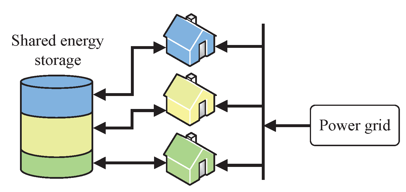
2.1. ES Sharing Model

The Shared ES: Consider an ES shared by multiple users, as shown in Figure 1. Each user is indexed by $i\in \mathcal{V}=\{1,\dots ,V\}$. The maximum and minimum amounts of energy stored in the ES are denoted by $C_{\max }$ and $C_{\min }$, respectively. The ES’s charging and discharging efficiencies are denoted by ${\eta }_{\mathrm{c}}$ and ${\eta }_{\mathrm{d}}$, respectively.

Time-of-Use Tariff: It is considered that users pay for electricity from the grid according to a TOU tariff [10,16]. Figure 2 shows a TOU tariff for residential consumers, which is provided by PG&E [21], an energy company in California. The TOU tariff divides a day into three periods: off-peak period (21:00–10:00), peak period 1 (10:00–13:00 and 19:00–21:00), and peak period 2 (13:00–19:00). The corresponding electricity prices are denoted by $P_{\mathrm{off}}$, $P_1^{\mathrm{pk}}$, and $P_2^{\mathrm{pk}}$, respectively. It is considered that the time periods and corresponding prices are unchanged every day. Given a TOU tariff, users can charge the ES in off-peak periods and discharge the ES to serve loads in peak periods. This prevents from buying grid energy at high prices, reducing electricity bills. For a TOU tariff, each peak period is indexed by $j\in \mathcal{J}=\{1,\dots ,J\}$. In the case of Figure 2, we have $J=2$.

Load Shifting Cost: To lower electricity bills, users desire to buy ES capacity to shift loads to off-peak periods. Users can change their capacity purchase decisions every round, and each round contains 24 h, as shown in Figure 2. To allow users to have sufficient time to charge the ES, we set that a round starts at the beginning of an off-peak period. Each round is indexed by $t\in \mathcal{T}=\{1,\dots ,T\}$. At the beginning of round t, user i makes a decision ${\mathit{c}}_{i,t}=[c_{i,1,t},\dots ,c_{i,J,t}]$ where $c_{i,j,t}$ denotes the amount of ES capacity (kWh) that user i buys for shifting the load of peak period j. Let $D_{i,j,t}$ stand for the original load (kWh) in peak period j, with $D_{i,j}^{\min }\le D_{i,j,t}\le D_{i,j}^{\max }$. The cost of user i during peak period j at round t is expressed by

$$\begin{array}{c}{P}_j^{\mathrm{pk}}max(D_{i,j,t}-c_{i,j,t},0).\end{array}$$

(1)

It is shown that if $c_{i,j,t}\ge D_{i,j,t}$, user i can use discharging energy to fully meet $D_{i,j,t}$ and then has zero cost in peak period j. If $c_{i,j,t}<D_{i,j,t}$, user i still needs to buy $D_{i,j,t}-c_{i,j,t}$ units of energy from the grid at price $P_j^{\mathrm{pk}}$.

Let $d_{i,j,t}$ denote the amount of energy that is shifted from peak period j to the off-peak period. In other words, to serve the load in peak period j, user i buys $d_{i,j,t}$ units of energy from the grid in the off-peak period and stores the energy in the ES. Due to energy loss of ES charging and discharging, $d_{i,j,t}$ is given by

$$\begin{array}{c}{d}_{i,j,t}=min\left(\frac{D_{i,j,t}}{{\eta }_{\mathrm{c}}{\eta }_{\mathrm{d}}},\frac{c_{i,j,t}}{{\eta }_{\mathrm{c}}{\eta }_{\mathrm{d}}}\right).\end{array}$$

(2)

Thus, the cost of user i in the off-peak period at round t is described by

$$\begin{array}{c}{P}_{\mathrm{off}}\left(\sum _{j\in \mathcal{J}}{d}_{i,j,t}+B_{i,t}-\frac{R_{i,t}}{{\eta }_{\mathrm{d}}}\right),\end{array}$$

(3)

where $B_{i,t}$ denote the original load in the off-peak period and $R_{i,t}$ is the energy left in the ES at the beginning of round t. As these two values do not relate to decision ${\mathit{c}}_{i,t}$, they are excluded in the following formulation.

Let $P_{\mathrm{es}}$ denote the price of ES capacity. The cost of user i for shifting the load of peak period j at round t is given by

$$\begin{array}{c}{l}_{i,j,t}\left(c_{i,j,t}\right)=P_{\mathrm{es}}{c}_{i,j,t}+P_j^{\mathrm{pk}}max(D_{i,j,t}-c_{i,j,t},0)+\frac{P_{\mathrm{off}}}{{\eta }_{\mathrm{c}}{\eta }_{\mathrm{d}}}min(D_{i,j,t},c_{i,j,t}),\end{array}$$

(4)

which includes three parts: the ES capacity purchase cost, the cost in peak period j, and the corresponding cost in the off-peak period. $l_{i,j,t}(·)$ is a piecewise-linear function, and it can also be written as

$$\begin{array}{c}{l}_{i,j,t}\left(c_{i,j,t}\right)=\left\{\begin{array}{cc}{\displaystyle \left(P_{\mathrm{es}}-P_j^{\mathrm{pk}}+\frac{P_{\mathrm{off}}}{{\eta }_{\mathrm{c}}{\eta }_{\mathrm{d}}}\right)c_{i,j,t}+P_j^{\mathrm{pk}}{D}_{i,j,t},}\hfill & c_{i,j,t}<D_{i,j,t},\hfill \\ {\displaystyle P_{\mathrm{es}}{c}_{i,j,t}+\frac{P_{\mathrm{off}}}{{\eta }_{\mathrm{c}}{\eta }_{\mathrm{d}}}{D}_{i,j,t},}\hfill & c_{i,j,t}\ge D_{i,j,t}.\hfill \end{array}\right.\end{array}$$

(5)

It is shown that $l_{i,j,t}(·)$ is convex in $c_{i,j,t}$ if $P_{\mathrm{es}}\le P_j^{\mathrm{pk}}-P_{\mathrm{off}}/\left({\eta }_{\mathrm{c}}{\eta }_{\mathrm{d}}\right)$. We consider that this inequality holds for the proposed ES sharing system. Intuitively, if ES price $P_{\mathrm{es}}$ is higher than arbitrage price $P_j^{\mathrm{pk}}-P_{\mathrm{off}}/\left({\eta }_{\mathrm{c}}{\eta }_{\mathrm{d}}\right)$, there is no incentive to encourage users to use the ES. To study ES sharing problems, this paper considers that the ES price is relatively low, i.e., the convexity of (5) holds. This facilitates the later cost minimization problem solving, and this is also the basic setting of other related works [10,16].

Satisfaction Degree: As shown in (5), the slopes of $l_{i,j,t}(·)$ are the same for all users, which means that given one unit of ES capacity, the amounts of cost reduction for all users may be the same. In fact, users who have high $D_{i,j,t}$ prefer the ES more than those with low $D_{i,j,t}$. To characterize the preference of user i for using ES, we introduce the following function to describe the satisfaction of a user getting $c_{i,j,t}$ units of ES capacity:

$$\begin{array}{c}{u}_{i,j,t}\left(c_{i,j,t}\right)=\omega ln\left(1+\frac{c_{i,j,t}}{D_{i,j,t}}\right),\end{array}$$

(6)

where $\omega$ is a parameter adjusting the importance of satisfaction. The reason for using (6) is that it can describe two features of the satisfaction of a user. First, the growth of satisfaction normally gets slow as the obtained ES capacity goes up, i.e., the marginal satisfaction decreases. Second, $c_{i,j,t}=D_{i,j,t}$ is the best capacity allocation for each user, so we set that all users have the same satisfaction if $c_{i,j,t}=D_{i,j,t}$, i.e., $u_{1,j,t}\left(D_{1,j,t}\right)=\dots =u_{V,j,t}\left(D_{V,j,t}\right)$. Figure 3 illustrates the two features of (6). Logarithmic satisfaction functions are widely used in related literature [22,23]. We can use other forms of satisfaction functions (e.g., quadratic functions [8,24]) as long as they have the two aforementioned properties.

Capacity Constraint: Because of the loss of charging/discharging, the available capacity of the shared ES is $C_{\mathrm{es}}={\eta }_{\mathrm{c}}{\eta }_{\mathrm{d}}(C_{\max }-C_{\min })$. The capacity allocation should satisfy

$$\begin{array}{c}\sum _{i\in \mathcal{V}}\sum _{j\in \mathcal{J}}{c}_{i,j,t}\le C_{\mathrm{es}}.\end{array}$$

(7)

Long-Term Budget Balance: Let $U_i$ denote the average budget that user i plans to spend on using the ES per round. Budget balance means that the actual expense is no more than the budget. Users do not need to achieve budget balance at each round, but they desire to achieve it in the long term. The long-term budget balance constraint for user i is given by

$$\begin{array}{c}\sum _{t\in \mathcal{T}}\left(P_{\mathrm{es}}\sum _{j\in \mathcal{J}}{c}_{i,j,t}-U_i\right)\le 0.\end{array}$$

(8)

2.2. System Cost Minimization

The total cost of user i for peak period j at round t is load shifting cost (5) minus satisfaction degree (6), denoted as $f_{i,j,t}\left(c_{i,j,t}\right)=l_{i,j,t}\left(c_{i,j,t}\right)-u_{i,j,t}\left(c_{i,j,t}\right)$. Define the total cost of user i at round t as $f_{i,t}\left({\mathit{c}}_{i,t}\right)={\sum }_{j\in \mathcal{J}}{f}_{i,j,t}\left(c_{i,j,t}\right)$. The ES sharing system minimizes the total costs of all users $i\in \mathcal{V}$ over T rounds. The system cost minimization problem is given by

$$\begin{array}{cc}\hfill \mathrm{P}1:\underset{\left\{{\mathit{c}}_t\right\}}{min}& \sum _{t\in \mathcal{T}}\sum _{i\in \mathcal{V}}{f}_{i,t}\left({\mathit{c}}_{i,t}\right),\hfill \end{array}$$

(9a)

$$\begin{array}{cc}\hfill \mathrm{s}.\mathrm{t}.& \sum _{i\in \mathcal{V}}{\mathbf{1}}^{\top }{\mathit{c}}_{i,t}\le C_{\mathrm{es}},\forall t\in \mathcal{T},\hfill \end{array}$$

(9b)

$$\begin{array}{c}{c}_{i,j,t}\ge 0,\forall i\in \mathcal{V},\forall j\in \mathcal{J},\forall t\in \mathcal{T},\hfill \end{array}$$

(9c)

$$\begin{array}{c}\sum _{t\in \mathcal{T}}(P_{\mathrm{es}}{\mathbf{1}}^{\top }{\mathit{c}}_{i,t}-U_i)\le 0,\forall i\in \mathcal{V},\hfill \end{array}$$

(9d)

where ${\mathit{c}}_t=[{\mathit{c}}_{1,t},\dots ,{\mathit{c}}_{V,t}]$ is the capacity allocation decision for round t. All vectors defined in this paper are column vectors. (7) and (8) are written as (9b) and (9d), respectively, using ${\mathit{c}}_{i,t}=[c_{i,1,t},\dots ,c_{i,J,t}]$ and $\mathbf{1}=[1,\dots ,1]\in {\mathbb{R}}^J$.

The challenge of solving P1 is twofold: 1) Peak load data ${\left\{D_{i,j,t}\right\}}_{i\in \mathcal{V},j\in \mathcal{J}}$ is fully disclosed at the end of round t. The load data relates to the user cost functions. In other words, the optimal allocation sequence $\{{\mathit{c}}_1^{*},\dots ,{\mathit{c}}_T^{*}\}$ is attainable only at the end of the Tth round, at which ${\left\{f_{i,t}(·)\right\}}_{i\in \mathcal{V},t\in \mathcal{T}}$ is completely known. Thus, only offline approaches can optimally solve P1, using historical or predictive load data. 2) The objective function of P1 is the sum of multiple piecewise functions. If the number of rounds T and the number of users V are very large, the number of pieces of P1 objective function is huge. In this case, it is impractical to get the exact expression of P1 objective function even though we assume that ${\left\{f_{i,t}(·)\right\}}_{i\in \mathcal{V},t\in \mathcal{T}}$ are known in advance.

3. Online Convex Optimization

Considering the above challenges, we solve P1 using online convex optimization, which is specified to multi-round online learning problems with convex (or concave) objective functions [17,18]. Specifically, we define $f_t\left(\mathit{c}\right)={\sum }_{i\in \mathcal{V}}{f}_{i,t}\left({\mathit{c}}_i\right)$ and $\mathcal{C}=\{\mathit{c}\in {\mathbb{R}}^{JV}:{\sum }_{i\in \mathcal{V}}{\mathbf{1}}^{\top }{\mathit{c}}_i\le C_{\mathrm{es}},c_{i,j}\ge 0,\forall i\in \mathcal{V},j\in \mathcal{J}\}$. At each round of online convex optimization, a learner selects decision ${\mathit{c}}_t$ from convex set $\mathcal{C}$ at the beginning of round t. At the end of round t, peak load data ${\left\{D_{i,j,t}\right\}}_{i\in \mathcal{V},j\in \mathcal{J}}$ is revealed, and the learner observes loss $f_t\left({\mathit{c}}_t\right)$. By employing online convex optimization, day-ahead load forecasting for each individual user is not required. In addition, P1 is decomposed into a series of one-round problems, reducing computational complexity.

3.1. Performance Metrics

We desire an online learning algorithm that produces a capacity allocation decision based on load data from previous rounds. To evaluate performance of the algorithm, two metrics are introduced: regret and constraint violation [18]. The regret after T rounds is defined as

$$\begin{array}{c}R\left(T\right)=\sum _{t=1}^T{f}_t\left({\mathit{c}}_t\right)-\sum _{t=1}^T{f}_t\left({\mathit{c}}^{*}\right),\end{array}$$

(10)

where ${\mathit{c}}^{*}$ is a fixed optimal solution to the following problem:

$$\begin{array}{c}\underset{\mathit{c}\in \mathcal{C}}{min}\sum _{t=1}^T{f}_t\left(\mathit{c}\right),\mathrm{s}.\mathrm{t}.P_{\mathrm{es}}{\mathbf{1}}^{\top }{\mathit{c}}_i\le U_i,\forall i\in \mathcal{V}.\end{array}$$

(11)

Regret $R\left(T\right)$ gives the difference between the cumulative loss of online decisions ${\left\{{\mathit{c}}_t\right\}}_{t\in \mathcal{T}}$ and that of the best fixed decision in hindsight. Note that computing ${\mathit{c}}^{*}$ requires complete load data of T rounds. In addition, ${\mathit{c}}^{*}$ is only attainable in theory. In the case of a very large T, it is impractical to optimally solve problem (11) as there are too many pieces of the objective function. An online algorithm aims at producing a sequence of decisions such that $R\left(T\right)$ grows sub-linearly with respect to T, leading to zero average regret, i.e., ${lim}_{T\to \infty }R\left(T\right)/T=0$.

In online convex optimization, capacity allocation is chosen from a fixed set $\mathcal{C}$, which does not involve time-coupling constraint (8). Thus, we need another metric to measure the constraint violation of budget balance. The constraint violation of user i after T rounds is defined as

$$\begin{array}{c}{W}_i\left(T\right)=\sum _{t=1}^T{h}_i\left({\mathit{c}}_{i,t}\right)=\sum _{t=1}^T(P_{\mathrm{es}}{\mathbf{1}}^{\top }{\mathit{c}}_{i,t}-U_i).\end{array}$$

(12)

We also desire that an online algorithm can ensure a sub-linear $W_i\left(T\right)$ so that average constraint violation goes to zero, i.e., ${lim}_{T\to \infty }{W}_i\left(T\right)/T=0$

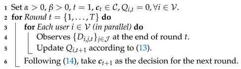
3.2. Online Algorithm

Based on [18], we develop an online algorithm to solve P1 round by round. First, a virtual queue $Q_i$ is used to measure constraint violation of user i, which is defined as

$$\begin{array}{c}{Q}_{i,t+1}=max\{Q_{i,t}+2\beta h_i\left({\mathit{c}}_{i,t}\right),0\},\end{array}$$

(13)

where $\beta >0$ is a predefined parameter, and $h_i\left({\mathit{c}}_{i,t}\right)$ is the constraint violation of user i at t, as shown in (12). $h_i\left({\mathit{c}}_{i,t}\right)\le 0$ implies that user i achieves budget balance at t. $h_i\left({\mathit{c}}_{i,t}\right)>0$ means that the budget-balance constraint is violated, increasing the virtual queue backlog. This would give a signal to the algorithm for adjusting allocation strategies. Then, we define ${\mathit{q}}_{i,t}=[Q_{i,t},\dots ,Q_{i,t}]\in {\mathbb{R}}^J$ and ${\mathit{q}}_t=[{\mathit{q}}_{1,t},\dots ,{\mathit{q}}_{V,t}]$. Given ${\mathit{q}}_t$ and ${\left\{D_{i,j,t}\right\}}_{i\in \mathcal{V},j\in \mathcal{J}}$, the ES capacity allocation for round $t+1$ is determined by

$$\begin{array}{c}{\mathit{c}}_{t+1}=\underset{\mathit{c}\in \mathcal{C}}{argmin}\parallel \mathit{c}-\left({\mathit{c}}_t-\frac{1}{2\alpha }{\mathit{d}}_t\right){\parallel }_2^2,\end{array}$$

(14)

where $\alpha >0$ is a parameter and ${\mathit{d}}_t=\beta P_{\mathrm{es}}{\mathit{q}}_t+\nabla f_t\left({\mathit{c}}_t\right)$. Here, $\nabla f_t\left({\mathit{c}}_t\right)=[\dots \nabla f_{i,j,t}\left(c_{i,j,t}\right),\dots ]$ denotes the gradient of $f_t(·)$ at ${\mathit{c}}_t$. Note that at the end of round t, both $f_t(·)$ and ${\mathit{c}}_t$ are known. Thus, we directly have $\nabla f_{i,j,t}\left(c_{i,j,t}\right)=P_{\mathrm{es}}-P_j^{\mathrm{pk}}+P_{\mathrm{off}}/\left({\eta }_{\mathrm{c}}{\eta }_{\mathrm{d}}\right)-\omega {(c_{i,j,t}+D_{i,j,t})}^{-1}$ if $c_{i,j,t}<D_{i,j,t}$ and $\nabla f_{i,j,t}\left(c_{i,j,t}\right)=P_{\mathrm{es}}-\omega {(c_{i,j,t}+D_{i,j,t})}^{-1}$ if $c_{i,j,t}\ge D_{i,j,t}$. Therefore, P1 has been decomposed into a series of one-round quadratic programming problems (14), avoiding dealing with the piecewise issue of P1.

The proposed online capacity allocation algorithm is summarized in Algorithm 1. At the end of round t, we observe peak loads ${\left\{D_{i,j,t}\right\}}_{i\in \mathcal{V},j\in \mathcal{J}}$, based on which we predict capacity allocation ${\mathit{c}}_{t+1}$ without knowing load data of round $t+1$. According to [18], parameter $\alpha$ is used for scaling norm $\parallel \mathit{c}-{\mathit{c}}_t{\parallel }_2^2$, and parameter $\beta$ is used for scaling constraint violation $h_i\left({\mathit{c}}_{i,t}\right)$. $\alpha$ and $\beta$ relate to the performance of the online algorithm. The following proposition shows that by setting $\alpha$ and $\beta$ appropriately, the resulting online decisions can ensure a $O\left(\sqrt{T}\right)$ regret bound and infinite constraint violation.

Algorithm 1: Online algorithm for solving P1

Proposition 1.

By setting $\alpha =\frac{1}{2}(P_{\mathrm{es}}^2+1)\sqrt{T}$ and $\beta =T^{1/4}$, the ES capacity allocation decision sequence $\{{\mathit{c}}_1,\dots ,{\mathit{c}}_T\}$ returned by Algorithm 1 guarantees

$$\begin{array}{cc}\hfill R\left(T\right)\le & \left[(3J{P}_{\mathrm{es}}^2+1)C_{\mathrm{es}}^2+2\Gamma +\Lambda \right]\sqrt{T},\hfill \end{array}$$

(15)

$$\begin{array}{cc}\hfill W_i\left(T\right)\le & \frac{1}{\epsilon }\left[(2J{P}_{\mathrm{es}}^2+1)C_{\mathrm{es}}^2+\Gamma +4C_{\mathrm{es}}\sqrt{\Lambda }\right]+2\sqrt{J{P}_{\mathrm{es}}^2{C}_{\mathrm{es}}^2+\Gamma },\forall i\in \mathcal{V},\hfill \end{array}$$

(16)

where $\Gamma ={\sum }_{i\in \mathcal{V}}{U}_i^2$, $\Lambda =\frac{1}{2}{\sum }_{i\in \mathcal{V}}{\sum }_{j\in \mathcal{J}}{\Lambda }_{i,j}$, ${\Lambda }_{i,j}=max\{{([P_{es}-P_j^{pk}+P_{off}/({\eta }_c{\eta }_d)]-\omega D_{i,j}^{min})}^2,P_{es}^2+\frac{1}{4}{(\omega /D_{i,j}^{min})}^2\}$, and $\epsilon >0$.

Proof of Proposition 1.

The proof follows from the analysis in [18], where the following assumptions are made.

• There exists $E>0$ such that $\parallel \nabla f_t{\left(\mathit{c}\right)\parallel }_2^2\le E,\forall \mathit{c}\in \mathcal{C},t\in \mathcal{T}$.
• Define $\mathit{h}\left(\mathit{c}\right)=[h_1\left({\mathit{c}}_1\right),\dots ,h_V\left({\mathit{c}}_V\right)]$. There exists $H>0$ such that ${\parallel \mathit{h}\left(\mathit{c}\right)-\mathit{h}\left(\mathit{e}\right)\parallel }_2^2\le H{\parallel \mathit{c}-\mathit{e}\parallel }_2^2,\forall \mathit{c},\mathit{e}\in \mathcal{C}$.
• There exists $G>0$ such that ${\parallel \mathit{h}\left(\mathit{c}\right)\parallel }_2^2\le G,\forall \mathit{c}\in \mathcal{C}$.
• There exists $K>0$ such that ${\parallel \mathit{c}-\mathit{e}\parallel }_2^2\le K,\forall \mathit{c},\mathit{e}\in \mathcal{C}$.
• There exist $\epsilon >0$ and $\widehat{\mathit{c}}\in \mathcal{C}$ such that $h_i\left({\widehat{\mathit{c}}}_i\right)\le -\epsilon ,\forall i\in \mathcal{V}$.

In the assumptions, E, H, G, K, and $\epsilon$ are constants. According to Theorems 1 and 2 in [18], if the above five assumptions hold, we have $R\left(T\right)\le [\frac{1}{2}(H+1)K+2G+\frac{1}{2}E]\sqrt{T}$ and $W_i\left(T\right)\le 2\sqrt{G}+\frac{1}{\epsilon }[\frac{1}{2}(H+1)K+G+2\sqrt{EK}]$ by setting $\beta =T^{1/4}$ and $\alpha =\frac{1}{2}(H+1)\sqrt{T}$.

In the following, we prove that the proposed ES sharing system satisfies the above assumptions. Using the following results, (15) and (16) can be obtained.

• If $c_{i,j,t}<D_{i,j,t}$, then ${(\nabla f_{i,j,t}\left(c_{i,j,t}\right))}^2\le {\{[P_{\mathrm{es}}-P_j^{\mathrm{pk}}+P_{\mathrm{off}}/({\eta }_{\mathrm{c}}{\eta }_{\mathrm{d}})]-\omega /D_{i,j}^{\min }\}}^2$. If $c_{i,j,t}\ge D_{i,j,t}$, then ${(\nabla f_{i,j,t}\left(c_{i,j,t}\right))}^2\le P_{\mathrm{es}}^2+(1/4){(\omega /D_{i,j}^{\min })}^2$. Combining these two cases, we have $\parallel \nabla f_t\left({\mathit{c}}_t\right){\parallel }_2^2\le 2\Lambda$.
• According to the definition of $\mathit{h}\left(\mathit{c}\right)$, we can derive that $\parallel \mathit{h}\left({\mathit{c}}_t\right)-\mathit{h}\left({\mathit{e}}_t\right){\parallel }_2^2=P_{\mathrm{es}}^2{\sum }_{i\in \mathcal{V}}{[{\sum }_{j\in \mathcal{J}}(c_{i,j,t}-e_{i,j,t})]}^2\le P_{\mathrm{es}}^2{\sum }_{i\in \mathcal{V}}\left[J{\sum }_{j\in \mathcal{J}}{(c_{i,j,t}-e_{i,j,t})}^2\right]=J{P}_{\mathrm{es}}^2{\parallel {\mathit{c}}_t-{\mathit{e}}_t\parallel }_2^2$ where the inequality is obtained from Cauchy-Schwarz inequality.
• $\parallel \mathit{h}\left({\mathit{c}}_t\right){\parallel }_2^2\le P_{\mathrm{es}}^2{\sum }_{i\in \mathcal{V}}{\left({\sum }_{j\in \mathcal{J}}{c}_{i,j,t}\right)}^2+{\sum }_{i\in \mathcal{V}}{U}_i^2\le J{P}_{\mathrm{es}}^2{\sum }_{i\in \mathcal{V}}{\sum }_{j\in \mathcal{J}}{c}_{i,j,t}^2+{\sum }_{i\in \mathcal{V}}{U}_i^2\le J{P}_{\mathrm{es}}^2{C}_{\mathrm{es}}^2+{\sum }_{i\in \mathcal{V}}{U}_i^2$, where the second inequality is also derived from Cauchy-Schwarz inequality.
• ${\parallel \mathit{c}-\mathit{e}\parallel }_2^2\le {\sum }_{i\in \mathcal{V}}{\sum }_{j\in \mathcal{J}}{c}_{i,j,t}^2+{\sum }_{i\in \mathcal{V}}{\sum }_{j\in \mathcal{J}}{e}_{i,j,t}^2\le {\left({\sum }_{i\in \mathcal{V}}{\sum }_{j\in \mathcal{J}}{c}_{i,j,t}\right)}^2+{\left({\sum }_{i\in \mathcal{V}}{\sum }_{j\in \mathcal{J}}{e}_{i,j,t}\right)}^2\le 2C_{\mathrm{es}}^2$.
• There exists ${\widehat{\mathit{c}}}_i$ such that $h_i\left({\widehat{\mathit{c}}}_i\right)=P_{\mathrm{es}}{\sum }_{j\in \mathcal{J}}{\widehat{c}}_{i,j,t}-U_i<0$. Thus, the constant $\epsilon >0$ exists such that $h_i\left({\widehat{\mathit{c}}}_i\right)\le -\epsilon$.

□

4. Distributed Implementation

If Algorithm 1 is implemented in a center, the center has to aggregate all load data from all users. However, due to privacy issues, users may not be willing to submit their load data to others. Therefore, this section designs a distributed implementation of Algorithm 1. In the distributed implementation, each user carries out local computation based on its load data and communicates with its neighbors via a P2P network without a center.

4.1. Network Problem

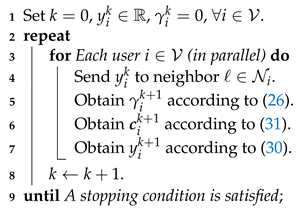
P2P Network Model: Consider that each user corresponds to a node in a P2P network. The P2P network can be abstracted as an undirected graph $\mathcal{G}=\{\mathcal{V},\mathcal{E}\}$, where $\mathcal{E}$ is the set of edges. Each edge, indexed by $(i,\ell )\in \mathcal{E}$, represents a bidirectional communication link between user i and user ℓ. The set of neighbors of user i is denoted by ${\mathcal{N}}_i=\{\ell :(i,\ell )\in \mathcal{E}\}$. Users only communicate with their neighbors. The topology of the P2P network can be arbitrary as long as it is connected. Compared to star networks where a center directly communicates with all users [25], P2P networks are more scalable and free from single-point failure [26]. Smart grid communication technologies [2,27,28] can implement secure information exchange between home energy users.

Problem at Round t: Let ${\mathit{v}}_t=[{\mathit{v}}_{1,t},\dots ,{\mathit{v}}_{V,t}]={\mathit{c}}_t-\frac{1}{2\alpha }{\mathit{d}}_t$, where ${\mathit{v}}_{i,t}={\mathit{c}}_{i,t}-\frac{1}{2\alpha }\left[\nabla f_{i,t}\left({\mathit{c}}_{i,t}\right)+\beta P_{\mathrm{es}}{\mathit{q}}_{i,t}\right]$. The problem in (14) can be written as

$$\begin{array}{cc}\hfill \mathrm{P}2:\underset{\mathit{c}}{min}& \sum _{i\in \mathcal{V}}{\parallel {\mathit{c}}_i-{\mathit{v}}_{i,t}\parallel }_2^2,\hfill \end{array}$$

(17a)

$$\begin{array}{cc}\hfill \mathrm{s}.\mathrm{t}.& \sum _{i\in \mathcal{V}}{\mathbf{1}}^{\top }{\mathit{c}}_i\le C_{\mathrm{es}},\hfill \end{array}$$

(17b)

$$\begin{array}{c}{c}_{i,j}\ge 0,\forall i\in \mathcal{V},\forall j\in \mathcal{J}.\hfill \end{array}$$

(17c)

Note that at the end of round t, user i knows ${\mathit{v}}_{i,t}$. In addition, attaining ${\mathit{v}}_{i,t}$ only requires local data of user i. (17b) is the global constraint coupling all users. In the following, we focus on the case that (17b) is binding. If (17b) is unbinding, P2 would be inherently separable.

P2P Network Problem: Next, we transform P2 into a network problem solvable in a P2P network. Let y be the Lagrange multiplier of (17b). The Lagrangian dual problem of P2 can be equivalently described as

$$\begin{array}{c}\hfill \underset{y}{min}\sum _{i\in \mathcal{V}}{\varphi }_i\left(y\right)+C_{\mathrm{es}}y,\end{array}$$

(18)

where

$$\begin{array}{c}\hfill {\varphi }_i\left(y\right)=\underset{{\mathit{c}}_i}{max}-{\parallel {\mathit{c}}_i-{\mathit{v}}_{i,t}\parallel }_2^2-y{\mathbf{1}}^{\top }{\mathit{c}}_i.\end{array}$$

(19)

Since P2 is a convex minimization with an affine constraint, the duality gap is zero [29,30]. This means that solving (18) is equivalent to solving P2. Let each user i manage a copy of y, denoted as $y_i$ [31]. Define $\mathit{y}={\left\{y_i\right\}}_{i\in \mathcal{V}}$ and $\mathit{\mu }={\left\{{\left\{{\mu }_{i\ell }\right\}}_{\ell \in {\mathcal{N}}_i}\right\}}_{i\in \mathcal{V}}$. Problem (18) can be transformed to the following P2P network problem:

$$\begin{array}{cc}\hfill \mathrm{P}3:\underset{\mathit{y},\mathbf{\mu }}{min}& \sum _{i\in \mathcal{V}}\left({\varphi }_i\left(y_i\right)+\frac{C_{\mathrm{es}}}{V}{y}_i\right),\hfill \end{array}$$

(20a)

$$\begin{array}{cc}\hfill \mathrm{s}.\mathrm{t}.& y_i={\mu }_{i\ell },y_{\ell }={\mu }_{i\ell },\forall \ell \in {\mathcal{N}}_i,i\in \mathcal{V},\hfill \end{array}$$

(20b)

where ${\left\{{\mu }_{i\ell }\right\}}_{\ell \in {\mathcal{N}}_i}$ are slack variables managed by user i. (20b) are consensus constraints, ensuring $y_1=y_2=\dots =y_V$. Thus, P3 is equivalent to problem (18).

4.2. ADMM Algorithm

In the following, we employ ADMM to solve P3 in a distributed manner. Let ${\lambda }_{i\ell }^{\prime }$ and ${\lambda }_{i\ell }^{″}$ be the Lagrange multipliers of (20b). Define $\mathit{\lambda }={\{{\{{\lambda }_{i\ell }^{\prime },{\lambda }_{i\ell }^{″}\}}_{\ell \in {\mathcal{N}}_i}\}}_{i\in \mathcal{V}}$. The augmented Lagrangian function of P3 is given by

$$\begin{array}{cc}\hfill {\mathcal{L}}_t(\mathit{y},\mathbf{\mu },\mathbf{\lambda })& =\sum _{i\in \mathcal{V}}\left({\varphi }_i\left(y_i\right)+\frac{C_{\mathrm{es}}}{V}{y}_i\right)+\sum _{i\in \mathcal{V}}\sum _{\ell \in {\mathcal{N}}_i}\left({\lambda }_{i\ell }^{\prime }(y_i-{\mu }_{i\ell })+{\lambda }_{i\ell }^{″}(y_{\ell }-{\mu }_{i\ell })\right)\hfill \\ & +\frac{\rho }{2}\sum _{i\in \mathcal{V}}\sum _{\ell \in {\mathcal{N}}_i}\left({(y_i-{\mu }_{i\ell })}^2+{(y_{\ell }-{\mu }_{i\ell })}^2\right),\hfill \end{array}$$

(21)

where $\rho$ is a penalty parameter. Use k to denote the number of iterations. Iterative steps of standard ADMM [19] for solving P3 are as follows:

$$\begin{array}{cc}\hfill {\mathit{y}}^{k+1}=& arg\underset{\mathit{y}}{min}{\mathcal{L}}_t(\mathit{y},{\mathbf{\mu }}^k,{\mathbf{\lambda }}^k),\hfill \end{array}$$

(22)

$$\begin{array}{cc}\hfill {\mathbf{\mu }}^{k+1}=& arg\underset{\mathbf{\mu }}{min}{\mathcal{L}}_t({\mathit{y}}^{k+1},\mathbf{\mu },{\mathbf{\lambda }}^k),\hfill \end{array}$$

(23)

$$\begin{array}{cc}\hfill {\lambda }_{i\ell }^{\prime ,k+1}=& {\lambda }_{i\ell }^{\prime ,k}+\rho (y_i^{k+1}-{\mu }_{i\ell }^{k+1}),\hfill \end{array}$$

(24)

$$\begin{array}{cc}\hfill {\lambda }_{i\ell }^{″,k+1}=& {\lambda }_{i\ell }^{″,k}+\rho (y_{\ell }^{k+1}-{\mu }_{i\ell }^{t+1}).\hfill \end{array}$$

(25)

Equations (22)–(25) can be further simplified using the properties of P3. From the definition of $\mathit{\mu }$ and (23), we can derive ${\mu }_{\ell i}^k={\mu }_{i\ell }^k$. Besides, according to the analysis of [32], we have ${\lambda }_{i\ell }^{\prime ,k}={\lambda }_{\ell i}^{″,k}=-{\lambda }_{i\ell }^{″,k}=-{\lambda }_{\ell i}^{\prime ,k},\forall k$ if we initialize ${\mathit{\lambda }}^0=\mathbf{0}$. Then, by defining ${\gamma }_i=2{\sum }_{\ell \in {\mathcal{N}}_i}{\lambda }_{i\ell }^{\prime ,k}$, (22)–(25) are equivalent to the following [32]:

$$\begin{array}{cc}\hfill {\gamma }_i^{k+1}& ={\gamma }_i^k+\rho \sum _{\ell \in {\mathcal{N}}_i}(y_i^k-y_{\ell }^k),\hfill \end{array}$$

(26)

$$\begin{array}{cc}\hfill y_i^{k+1}& =arg\underset{y_i}{min}\left\{{\varphi }_i\left(y_i\right)+\frac{C_{\mathrm{es}}}{V}{y}_i+{\gamma }_i^{k+1}{y}_i+\rho \sum _{\ell \in {\mathcal{N}}_i}{\left[y_i-\frac{1}{2}(y_i^k+y_{\ell }^k)\right]}^2\right\},\hfill \end{array}$$

(27)

which show that P3 is split into multiple subproblems that can be solved by individual users $i\in \mathcal{N}$. Due to (19), y-update (27) involves a min-max problem. According to minimax theorem [33], the min-max problem of (27) is equivalent to the following max-min problem:

$$\begin{array}{c}\underset{{\mathit{c}}_i}{max}\underset{y_i}{min}\left\{-\parallel {\mathit{c}}_i-{\mathit{v}}_{i,t}{\parallel }_2^2-y_i{\mathbf{1}}^{\top }{\mathit{c}}_i+\frac{C_{\mathrm{es}}}{V}{y}_i+{\gamma }_i^{k+1}{y}_i+\rho \sum _{\ell \in {\mathcal{N}}_i}{\left[y_i-\frac{1}{2}(y_i^k+y_{\ell }^k)\right]}^2\right\}\\ \iff \underset{{\mathit{c}}_i}{max}\underset{y_i}{min}\{\rho |{\mathcal{N}}_i|{\left[y_i-\frac{1}{2\rho |{\mathcal{N}}_i|}\left({\mathbf{1}}^{\top }{\mathit{c}}_i-\frac{C_{\mathrm{es}}}{V}-{\gamma }_i^{k+1}+\rho \sum _{\ell \in {\mathcal{N}}_i}(y_i^k+y_{\ell }^k)\right)\right]}^2-{\parallel {\mathit{c}}_i-{\mathit{v}}_{i,t}\parallel }_2^2\end{array}$$

(28)

$$\begin{array}{c}-\frac{1}{4\rho |{\mathcal{N}}_i|}{\left[{\mathbf{1}}^{\top }{\mathit{c}}_i-\frac{C_{\mathrm{es}}}{V}-{\gamma }_i^{k+1}+\rho \sum _{\ell \in {\mathcal{N}}_i}(y_i^k+y_{\ell }^k)\right]}^2\}.\hfill \end{array}$$

(29)

From (29), we have the closed-form solution of $y_i$ given by

$$\begin{array}{c}\hfill y_i^{k+1}=\frac{1}{2\rho |{\mathcal{N}}_i|}\left({\mathbf{1}}^{\top }{\mathit{c}}_i^{k+1}-\frac{C_{\mathrm{es}}}{V}-{\gamma }_i^{k+1}+\rho \sum _{\ell \in {\mathcal{N}}_i}(y_i^k+y_{\ell }^k)\right).\end{array}$$

(30)

The outer maximizer of (29) can be obtained by

$$\begin{array}{c}{\mathit{c}}_i^{k+1}=arg\underset{{\mathit{c}}_i}{min}\left\{\parallel {\mathit{c}}_i-{\mathit{v}}_{i,t}{\parallel }_2^2+\frac{1}{4\rho |{\mathcal{N}}_i|}{\left[{\mathbf{1}}^{\top }{\mathit{c}}_i-\frac{C_{\mathrm{es}}}{V}-{\gamma }_i^{k+1}+\rho \sum _{\ell \in {\mathcal{N}}_i}(y_i^k+y_{\ell }^k)\right]}^2\right\},\end{array}$$

(31)

where ${\mathit{c}}_i$ is bounded by $c_{i,j}\ge 0,\forall j\in \mathcal{J}$.

Therefore, the ADMM-based distributed algorithm for solving P3 (and P2) is described by Algorithm 2. At each iteration, each user exchanges $y_i$ with its neighbors and updates three variables. The $\mathit{c}$-update (31) involves a quadratic programming problem, which can be solved efficiently. Algorithm 2 falls under dual consensus ADMM, and related convergence analysis can be found in [34]. Algorithm 2 is used to compute (14) at each round.

Algorithm 2: Distributed Algorithm for solving P3

5. Numerical Result

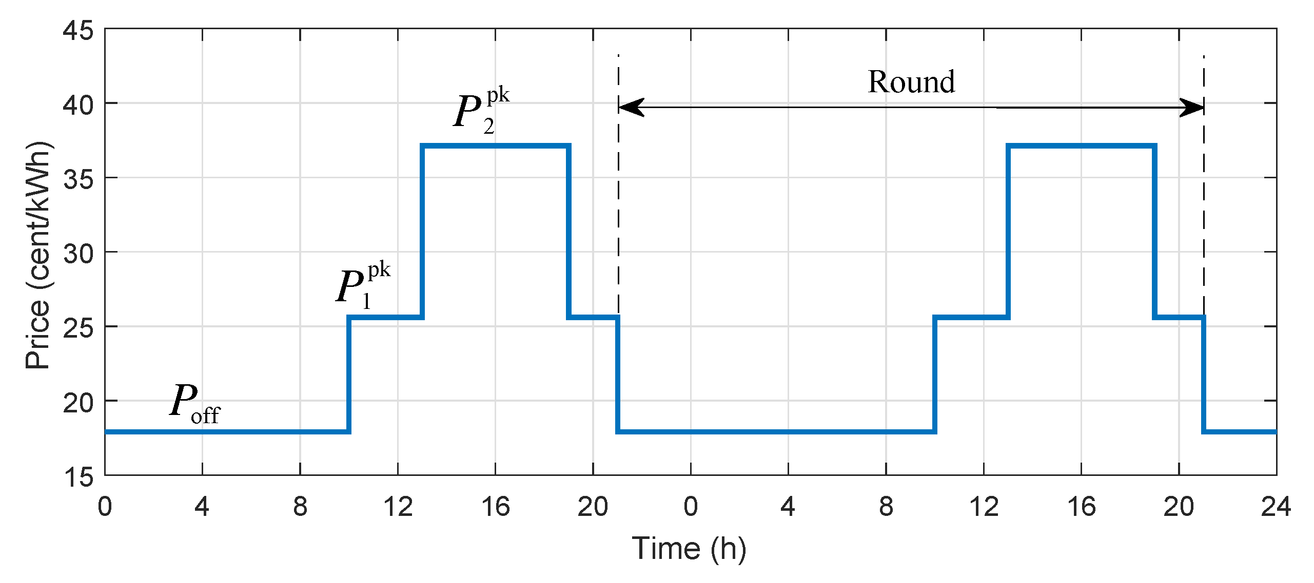
5.1. Simulation Setup

In the simulation, the residential TOU tariff shown in Figure 2 is used, in which $P_{\mathrm{off}}=17.918$ cent/kWh, $P_1^{\mathrm{pk}}=25.596$ cent/kWh, and $P_2^{\mathrm{pk}}=37.123$ cent/kWh [21]. We set the TOU tariff unchanged every day. The home load data is taken from Dataport database [20], which includes power data of Texas, Colorado, and California. Figure 4 shows a home’s load profiles of peak period 1 and peak period 2 in 2017. The peak load data is used to set $D_{i,j,t}$ in (5) and (6). We evaluate the proposed online approach in two systems: 10-home and 100-home systems. In the first system, 10 homes share an ES that has the following parameters: $C_{\max }=50$ kWh, $C_{\min }=\frac{1}{10}{C}_{\max }$, and ${\eta }_{\mathrm{d}}={\eta }_{\mathrm{c}}=0.95$. In the second system, 100 homes share an ES with $C_{\max }=200$ kWh (other parameters are the same as the first system). The price of ES capacity is set to be $P_{\mathrm{es}}\le P_1^{\mathrm{pk}}-P_{\mathrm{off}}/\left({\eta }_{\mathrm{c}}{\eta }_{\mathrm{d}}\right)$. The satisfaction parameter $\omega$ adjusts the trade-off between load shifting cost and satisfaction of a home, and we set $\omega =30$. A home’s budget is set to be uniformly distributed in $[0.1,0.5]$ $. The proposed online approach is tested for $T=365$ days (i.e., rounds). The communication network graph is generated following the method in [34]. Consider that nodes are randomly located in a 100 m × 100 m area. Let r denote the communication radius of each node. If the geographical distance between two homes is no more than r, a communication link is established between the two homes.

The proposed online approach is compared with the following benchmarks:

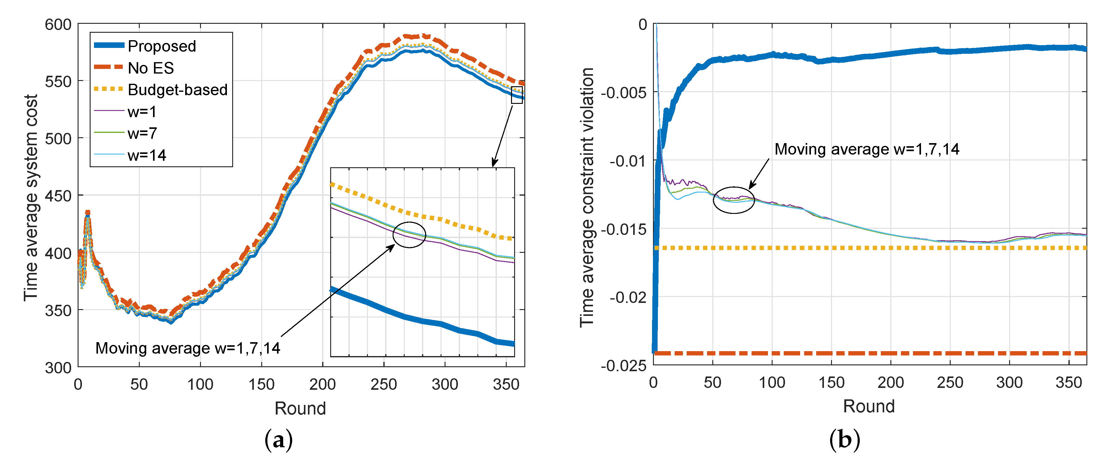
• No ES: In the case of no shared ES, users have to buy electricity from the grid to meet their immediate demands.
• Budget-based: This is a fixed ES capacity allocation approach based on users’ budgets. The amount of capacity allocated to user i for peak period j is given by

  $$\begin{array}{c}{c}_{i,j}=\frac{L_j}{{\displaystyle \sum _{j\in \mathcal{J}}{L}_j}}min\left\{\frac{U_i}{{\displaystyle \sum _{i\in \mathcal{V}}{U}_i}}{C}_{\mathrm{es}},\frac{U_i}{P_{\mathrm{es}}}\right\},\end{array}$$

  (32)

  where $L_j$ is the length of peak period j. Note that for each user i, we have $P_{\mathrm{es}}{\sum }_{j\in \mathcal{J}}{c}_{i,j}\le U_i$ which indicates that each user is budget-balanced.
• Moving Average: This is a time-variant ES capacity allocation approach based on moving average [35]. This approach is parameterized by a time window w. The allocation decision for round t will be determined based on the average peak loads from round $t-w$ to round $t-1$.
  Define

  $$\begin{array}{c}{\overline{D}}_{i,j,t}=\frac{1}{w}\sum _{\tau =t-w}^{t-1}{D}_{i,j,\tau }.\end{array}$$

  (33)
  The amount of capacity allocated to user i for peak period j for round t is given by

  $$\begin{array}{c}{c}_{i,j,t}=\frac{{\overline{D}}_{i,j,t}}{{\displaystyle \sum _{j\in \mathcal{J}}\sum _{i\in \mathcal{V}}{\overline{D}}_{i,j,t}}}{C}_{\mathrm{es}}.\end{array}$$

  (34)
  Note that users’ budgets are not considered in this approach, so budget balance may not be guaranteed.

5.2. ES Capacity Allocation Performance

The performance metrics for the proposed online approach are regret (10) and constraint violation (12). For the regret, it is impractical to attain the second term of (10) because of the huge number of pieces of the objective functions in problem (11). Fortunately, the second term of (10) is constant for different allocation approaches. Thus, it is feasible to compare different approaches by only using the first term of (10), i.e., the resultant system cost.

Figure 5 illustrates time average system costs and time average constraint violations of different ES capacity allocation approaches. As shown in Figure 5a, in the case of no ES, the system always incurs the highest cost. At the last 10 rounds (shown in the zoom-in box in Figure 5a), it is clear that the proposed online approach outperforms other benchmark approaches, having the lowest system cost. For the moving average approach, three time windows are selected, i.e., $w=1,7,14$. It is observed that the impact of time window selection is small. The budget balance constraint highly influences the system cost. Figure 5b shows the time average constraint violation of the user who has the highest violation, i.e., ${max}_{i\in \mathcal{V}}{W}_i\left(T\right)$. It is shown that the constraint violations are negative for all approaches, which means that all users are budget-balanced in all approaches. In the case of no ES, users do not spend on ES capacity so that the constraint violation is the lowest. In the proposed online approach, the constraint violation keeps negative and close to zero. This means that the proposed approach takes full advantage of the users with small budgets to reduce the system cost and meanwhile maintains users’ budget balance. In contrast, the budget-based and moving average approaches have lower constraint violations, which means that part of user budgets are not utilized to reduce system costs. Thus, their system costs are higher than that of the proposed approach. The 100-user system also has similar results, which are shown in Figure 6.

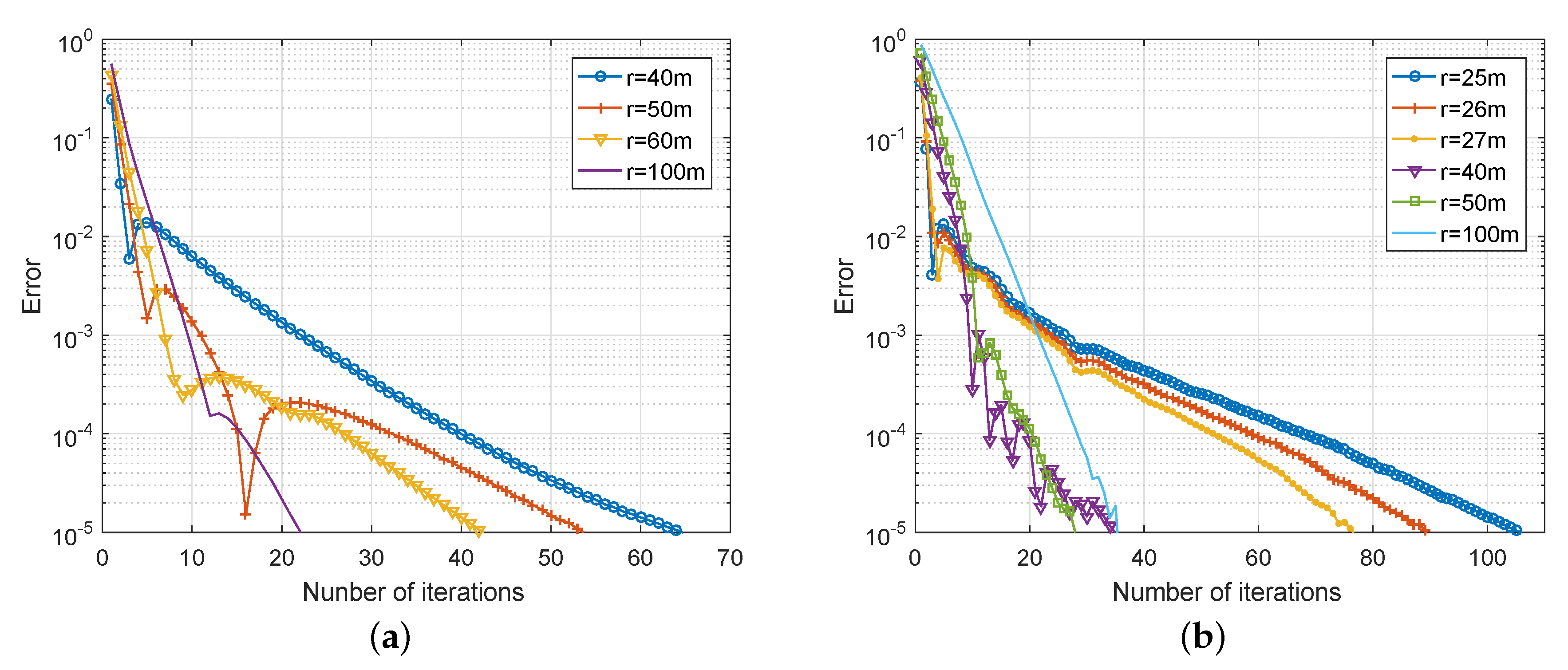
5.3. Convergence Performance

Here, we evaluate the convergence performance of Algorithm 2. Figure 7a shows the convergence rates in the 10-home system under different communication radii. The y axis, error, is defined as $|{\phi }^k-{\phi }^{*}|/{\phi }^{*}$, where ${\phi }^{*}$ denotes the optimal objective value of P2 and ${\phi }^k$ denotes the P2 objective value given by Algorithm 2 at the kth iteration. As shown in Figure 7a, as the communication radius r increases, the number of a node’s neighbors increases, which accelerates convergence. $r=100$ m corresponds to the case where a home is contactable to any other home, i.e., a complete graph. In the 100-home system, the density of nodes is higher. As shown in Figure 7b, when r is relative small (e.g., $r=25,26,27$ m), a small increment of r can significantly speed up convergence. When r is large (e.g., $r\ge 40$ m), each home already has a lot of neighbors. In this case, the increase of r does not accelerate convergence too much but stabilizes it. As long as the communication network is connected, Algorithm 2 is able to achieve convergence efficiently.

6. Conclusions

This paper studies ES capacity allocation using online convex optimization. Firstly, we model an ES sharing system, in which homes buy ES capacity to shift loads to off-peak periods. Secondly, an online capacity allocation algorithm is developed, which is able to minimize homes’ costs via learning from home load data. Thirdly, a distributed implementation of the online algorithm is proposed using ADMM framework. Finally, real-world home load data and a practical TOU tariff are used in the simulation. The results show that compared to other benchmark approaches, the proposed online approach has the lowest system cost while maintaining homes’ budget balance.

References

1. NIST Framework and Roadmap for Smart Grid Interoperability Standards, Release 3.0. Available online: http://dx.doi.org/10.6028/NIST.SP.1108r3 (accessed on 20 December 2018).
2. Liu, Y.; Yang, C.; Jiang, L.; Xie, S.; Zhang, Y. Intelligent edge computing for IoT-based energy management in smart cities. IEEE Netw. 2019, 33, 111–117. [Google Scholar] [CrossRef]
3. Guo, Y.; Pan, M.; Fang, Y. Optimal power management of residential customers in the smart grid. IEEE Trans. Parallel Distrib. Syst. 2012, 23, 1593–1606. [Google Scholar] [CrossRef]
4. Yang, C.; Lou, W.; Yao, J.; Xie, S. On charging scheduling optimization for a wirelessly charged electric bus system. IEEE Trans. Intell. Transp. Syst. 2018, 19, 1814–1826. [Google Scholar] [CrossRef]
5. Sun, S.; Dong, M.; Liang, B. Distributed real-time power balancing in renewable-integrated power grids with storage and flexible loads. IEEE Trans. Smart Grid 2016, 7, 2337–2349. [Google Scholar] [CrossRef]
6. Zhong, W.; Yu, R.; Xie, S.; Zhang, Y.; Yau, D.K.Y. On Stability and Robustness of Demand Response in V2G Mobile Energy Networks. IEEE Trans. Smart Grid 2018, 9, 3203–3212. [Google Scholar] [CrossRef]
7. Li, N.; Hedman, K.W. Economic assessment of energy storage in systems with high levels of renewable resources. IEEE Trans. Sustain. Energy 2015, 6, 1103–1111. [Google Scholar] [CrossRef]
8. Yang, C.; Yao, J.; Lou, W.; Xie, S. On demand response management performance optimization for microgrids under imperfect communication constraints. IEEE Internet Things J. 2017, 4, 881–893. [Google Scholar] [CrossRef]
9. Wang, Z.; Gu, C.; Li, F.; Bale, P.; Sun, H. Active demand response using shared energy storage for household energy management. IEEE Trans. Smart Grid 2013, 4, 1888–1897. [Google Scholar] [CrossRef]
10. Kalathil, D.; Wu, C.; Poolla, K.; Varaiya, P. The sharing economy for the electricity storage. IEEE Trans. Smart Grid 2018, 10, 556–567. [Google Scholar] [CrossRef]
11. Rahbar, K.; Moghadam, M.R.V.; Panda, S.K.; Reindl, T. Shared energy storage management for renewable energy integration in smart grid. In Proceedings of the 2016 IEEE Power & Energy Society Innovative Smart Grid Technologies Conference (ISGT), Minneapolis, MN, USA, 6–9 September 2016; pp. 1–5. [Google Scholar]
12. Rahbar, K.; Moghadam, M.R.V.; Panda, S.K.; Reindl, T. Energy management for demand responsive users with shared energy storage system. In Proceedings of the 2016 IEEE International Conference on Smart Grid Communications (SmartGridComm), Sydney, NSW, Australia, 6–9 November 2016; pp. 290–295. [Google Scholar]
13. Paridari, K.; Parisio, A.; Sandberg, H.; Johansson, K.H. Demand response for aggregated residential consumers with energy storage sharing. In Proceedings of the 54th IEEE Conference on Decision and Control (CDC), Osaka, Japan, 15–18 December 2015; pp. 2024–2030. [Google Scholar]
14. Zhao, D.; Wang, H.; Huang, J.; Lin, X. Pricing-based energy storage sharing and virtual capacity allocation. In Proceedings of the 2017 IEEE International Conference on Communications (ICC), Paris, France, 21–25 May 2017; pp. 1–6. [Google Scholar]
15. Dimitrov, P.; Piroddi, L.; Prandini, M. Distributed allocation of a shared energy storage system in a microgrid. In Proceedings of the 2016 American Control Conference (ACC), Boston, MA, USA, 6–8 July 2016; pp. 3551–3556. [Google Scholar]
16. Chakraborty, P.; Baeyens, E.; Poolla, K.; Khargonekar, P.P.; Varaiya, P. Sharing storage in a smart grid: A coalitional game approach. IEEE Trans. Smart Grid (Early Access) 2018. [Google Scholar] [CrossRef]
17. Shalev-Shwartz, S. Online learning and online convex optimization. Found. Trends Mach. Learn. 2012, 4, 107–194. [Google Scholar] [CrossRef]
18. Yu, H.; Neely, M.J. A low complexity algorithm with O ( T ) regret and finite constraint violations for online convex optimization with long term constraints. arXiv 2016, arXiv:1604.02218. [Google Scholar]
19. Boyd, S.; Parikh, N.; Chu, E.; Peleato, B.; Eckstein, J. Distributed optimization and statistical learning via the alternating direction method of multipliers. Found. Trends Mach. Learn. 2011, 3, 1–122. [Google Scholar] [CrossRef]
20. Dataport. Available online: https://www.dataport.cloud/ (accessed on 15 December 2018).
21. Pacific Gas & Electric - Tariffs. Available online: https://www.pge.com/tariffs/electric.shtml#RESELEC_TOU/ (accessed on 15 December 2018).
22. Maharjan, S.; Zhu, Q.; Zhang, Y.; Gjessing, S.; Basar, T. Dependable Demand Response Management in the Smart Grid: A Stackelberg Game Approach. IEEE Trans. Smart Grid 2013, 4, 120–132. [Google Scholar] [CrossRef]
23. Wu, Y.; Tan, X.; Qian, L.; Tsang, D.H.K.; Song, W.; Yu, L. Optimal pricing and energy scheduling for hybrid energy trading market in future smart grid. IEEE Trans. Ind. Inform. 2015, 11, 1585–1596. [Google Scholar] [CrossRef]
24. Zhong, W.; Xie, K.; Liu, Y.; Yang, C.; Xie, S. Topology-aware vehicle-to-grid energy trading for active distribution systems. IEEE Trans. Smart Grid 2019, 10, 2137–2147. [Google Scholar] [CrossRef]
25. Zhong, W.; Xie, K.; Liu, Y.; Yang, C.; Xie, S. Auction Mechanisms for Energy Trading in Multi-Energy Systems. IEEE Trans. Ind. Informat. 2018, 14, 1511–1521. [Google Scholar] [CrossRef]
26. Tsai, S.; Tseng, Y.; Chang, T. Communication-efficient distributed demand response: A randomized ADMM approach. IEEE Trans. Smart Grid 2017, 8, 1085–1095. [Google Scholar] [CrossRef]
27. Liu, Y.; Yu, R.; Pan, M.; Zhang, Y.; Xie, S. SD-MAC: Spectrum database-driven MAC protocol for cognitive machine-to-machine networks. IEEE Trans. Veh. Technol. 2017, 66, 1456–1467. [Google Scholar] [CrossRef]
28. Li, Z.; Yang, Z.; Xie, S.; Chen, W.; Liu, K. Credit-based payments for fast computing resource trading in edge-assisted internet of things. IEEE Internet Things J. (Early Access) 2019. [Google Scholar] [CrossRef]
29. Boyd, S.; Vandenberghe, L. Convex Optimization; Cambridge University Press: New York, NY, USA, 2004. [Google Scholar]
30. Yang, C.; Liu, Y.; Chen, X.; Zhong, W.; Xie, S. Efficient mobility-aware task offloading for vehicular edge computing networks. IEEE Access 2019, 7, 26652–26664. [Google Scholar] [CrossRef]
31. Zhong, W.; Yang, C.; Xie, K.; Xie, S.; Zhang, Y. ADMM-based distributed auction mechanism for energy hub scheduling in smart buildings. IEEE Access 2018, 6, 45635–45645. [Google Scholar] [CrossRef]
32. Mateos, G.; Bazerque, J.A.; Giannakis, G.B. Distributed sparse linear regression. IEEE Trans. Signal Process. 2010, 58, 5262–5276. [Google Scholar] [CrossRef]
33. Bertsekas, D.; Nedić, A.; Ozdaglar, A. Convex Analysis and Optimization; Athena Scientific Optimization and Computation Series; Athena Scientific: Belmont, MA, USA, 2003. [Google Scholar]
34. Chang, T.; Hong, M.; Wang, X. Multi-agent distributed optimization via inexact consensus ADMM. IEEE Trans. Signal Process. 2015, 63, 482–497. [Google Scholar] [CrossRef]
35. Hund, T.D.; Gonzalez, S.; Barrett, K. Grid-tied PV system energy smoothing. In Proceedings of the 35th IEEE Photovoltaic Specialists Conference, Honolulu, HI, USA, 20–25 June 2010; pp. 2762–2766. [Google Scholar]
Figure 1. An energy storage device shared by multiple residential energy users.
Energies 12 01642 g001
Figure 2. Residential time-of-use tariff provided by PG&E [21].
Energies 12 01642 g002
Figure 3. Examples of satisfaction functions with D i , j , t = 10 kWh and D i , j , t = 50 kWh.
Energies 12 01642 g003
Figure 4. Peak load data of a home during the year of 1 January–31 December 2017 [20].
Energies 12 01642 g004
Figure 5. Energy storage capacity allocation performances in the 10-home system. (a) Time average system cost. (b) The highest time average constraint violation of budget balance.
Energies 12 01642 g005
Figure 6. Energy storage capacity allocation performances in the 100-home system. (a) Time average system cost. (b) The highest time average constraint violation of budget balance.
Energies 12 01642 g006
Figure 7. Convergence performances in (a) the 10-home system and (b) the 100-home system with different communication radii.
Energies 12 01642 g007