Article

Day-Ahead Photovoltaic Forecasting: A Comparison of the Most Effective Techniques

1
Department of Energy, Politecnico di Milano, 20156 Milano, Italy
2
Department of Engineering and Architecture, Università degli Studi di Trieste, 34127 Trieste, Italy
3
Renewable Energy Laboratory, Jijel University, Jijel 18000, Algeria
*
Author to whom correspondence should be addressed.
Energies 2019, 12(9), 1621; https://doi.org/10.3390/en12091621
Submission received: 25 March 2019 / Revised: 12 April 2019 / Accepted: 23 April 2019 / Published: 29 April 2019
(This article belongs to the Special Issue Solar and Wind Power and Energy Forecasting)

Abstract

:
We compare the 24-hour ahead forecasting performance of two methods commonly used for the prediction of the power output of photovoltaic systems. Both methods are based on Artificial Neural Networks (ANN), which have been trained on the same dataset, thus enabling a much-needed homogeneous comparison currently lacking in the available literature. The dataset consists of an hourly series of simultaneous climatic and PV system parameters covering an entire year, and has been clustered to distinguish sunny from cloudy days and separately train the ANN. One forecasting method feeds only on the available dataset, while the other is a hybrid method as it relies upon the daily weather forecast. For sunny days, the first method shows a very good and stable prediction performance, with an almost constant Normalized Mean Absolute Error, NMAE%, in all cases (1% < NMAE% < 2%); the hybrid method shows an even better performance (NMAE% < 1%) for two of the days considered in this analysis, but overall a less stable performance (NMAE% > 2% and up to 5.3% for all the other cases). For cloudy days, the forecasting performance of both methods typically drops; the performance is rather stable for the method that does not use weather forecasts, while for the hybrid method it varies significantly for the days considered in the analysis.

1. Introduction

In 2017, global energy investment declined, with a fall of 2% with respect to the previous year, mainly due to lower production of coal, hydroelectric, and nuclear power [1]. On the other hand, renewables have shown unprecedented growth over the past few years because of a number of factors: climate change is now a major concern worldwide [2], air pollution in big cities (e.g. in China) has become a serious problem [3], the depletion of conventional energy resources shows that, continuing the current pattern of management, they could be largely exhausted by the end of the century [4], the cost of electricity from wind power and photovoltaics is diminishing [5], and the deployment of renewable-based power plants requires the least time among all power generation technologies [6]. In this framework, photovoltaic is the fastest-growing renewable technology and the sector with the largest investment [6].
As the amount of energy produced by PV systems is growing exponentially, the need to forecast their production is more critical than in the past, when PV plants were installed with a “fit and forget” approach. The production of solar plants is uncertain, especially due to the stochastic formation and movement of clouds in the sky. Thus, accurate forecasting models based on the use of field measurements and data from weather forecast providers [7] are needed in order to optimize the operation of these systems. The benefits of such models are manifold. Considering the point of view of the owners of residential and Commercial‒Industrial (C&I) PV plants, and specifically the possibility of operating in a grid-parity regime or better, accurate forecasts enable the maximization of the self-consumed energy and minimization of the Levelized Cost of the Energy produced (LCoE) [8,9]. Also, when residential and C&I systems operate as part of a microgrid, the power forecasts can be used as input for the Energy Management System (EMS) used to optimize the State of Charge (SoC) of the storage devices [10]. On the other hand, considering larger-scale plants and fuel parity [11], the managers of utility-scale PV plants use the forecasts to optimally plan the downtime of plants for maintenance purposes. Moreover, in countries with a day-ahead electricity market, forecast models allow for optimization of the schedule for the supply offers on the market, avoiding penalties and reduced revenues [12,13]. On the other hand, Distribution System Operators (DSOs) and Transmission System Operators (TSOs) also need reliable forecasts in order to handle the uncertainty and fluctuations of the PV distributed generators connected to their grids. The availability of reliable forecasts allows DSOs and TSOs to cope with the intermittent nature of PV plants, avoiding problems in balancing power generation and load demand [14], enhancing the stability of the system, and reducing the cost of ancillary services [15,16]. Accurate forecasts enhance reliability, and reduce costs by allowing efficient solar energy trading and more efficient and secure management of electricity grids [17]. In addition, forecasting leads to a lower number of units in hot standby and a reduced cost for the operation of the entire power system [18]. Incidentally, one should consider that PV plants can be aggregated in Virtual Power Plants (VPP). In this case, the variability of the solar radiation can impact to a lesser extent the power grid that the VPP is connected to; on the other hand, this type of aggregation—“behind the meter”—can cause errors in load forecasting [19,20].
Over the past few years, a very large number of forecasting techniques for PV power systems has been developed and presented in the literature. One classification of these forecasting methods is based on the forecast horizon, i.e., the amount of time between the actual time and the effective time of prediction [18]. Even if there is not any widely agreed upon classification criterion [14,16], a common classification is the following: long-term (1–10 years), mid-term (1 month–1 year), short-term (1 hour–1 week), very short (1 minute–a few minutes) [16]. The last two forecast horizons are also known as intraday [10], while the most important forecasting horizon is 24 h of the next day [12]. Different forecast horizons are best suited to different applications (e.g., residential, C&I, or utility-scale). For example, very short-term models are useful for power smoothing and real-time power dispatching. Short-term forecasters are used for automatic generation control, unit dispatching, load balancing and plant management, while longer forecast horizons are used by utilities for unit commitment, load balancing and scheduling. Finally, DSOs and TSOs use short and medium forecasters but also long-term horizons for planning their infrastructure [16]. Another classification is based on the method used to perform the forecast. This classification comprises three main families of forecasting techniques: statistical or time series-based methods, physical methods, and hybrid or ensemble methods.
Statistical methods are based on a sequence of observations of one or more parameters measured at successive instants in time [21]. These methods include different types of Artificial Neural Networks (ANN) such as Multilayer Perceptron (MLP) [22,23,24], Support Vector Machine (SVM) [25], Markov chain, Fourier Series, regression methods, persistence methods (mainly used as a benchmark to test other models), etc. These methods only rely on data that have been collected in the past and do not require any information regarding the PV systems or the location where they are installed. Among the statistical based-forecasters, ANNs and regression models are the most widely used. According to many authors and reviews, ANN-based forecasting is one of the most effective methods. This is due to the ability of ANNs to capture sharp changes in the input‒output relationship due to varying environmental conditions [16]. However, the main drawback is that ANNs require a large amount of data for the training process, a random initial dataset that may reduce the reliability of the forecasted results, and an accurate selection of the model architecture (i.e., number of hidden layers, neurons, etc.) [14]. Auto-Regressive Moving Average (ARMA) forecasters perform well when data are stationary, while Auto-Regressive Integrated Moving Average (ARIMA) models perform well with non-stationary time series [26]. The drawback of ARIMA methods is that they are computationally more intensive than ARMA. According to the results of [16], ANNs demonstrate higher accuracy than ARMA and ARIMA and outperform other statistical methods in terms of accuracy and adaptability under uncertain meteorological conditions. However, the grouping of daily weather conditions [27,28,29,30,31] into sunny, cloudy and rainy days improves the performance of any statistical-based forecast [14,16,24,32]. This approach is mainly used for very short and short horizon applications [14,33] and represents the majority of forecast techniques currently utilized [34].
Physical methods, mainly used for applications ranging from very short to long horizons, consist of a set of mathematical equations that describe the physical state and dynamic motion of the atmosphere [35]. These methods are mainly based on Numerical Weather Prediction (NPW), Sky Imagery and Satellite Imaging [36]. They can be classified as global and mesoscale physical methods, based on the portion of the simulated atmosphere—which can be at a worldwide scale or include a limited area [37]. With reference to the forecast of the power produced by PV plants, only mesoscale models should be used; the main shortcoming of such models is that a resolution of only up to 16–50 km can be attained [38]. Another drawback of physical methods is that their performance is higher when weather conditions are stable [39] and that the accuracy is strongly affected by sharp changes in the meteorological variables [16].
Hybrid methods are a combination of any of the previous methods. The idea is to mix different models with unique features to address the limitations of individual techniques, thus enhancing the forecast performance [40,41,42]. Generally, the computational complexity increases [14]. The most common examples reported in the literature are combinations of ANN- and NPW-based models [12,43,44,45], and also of SARIMA and SVM [46]. The performance of hybrid models depends on the performance of the single models, and these models should be specifically designed for a particular plant and location [36]. Hybrid methods where numerical weather forecasts are used together with the use of historical data of the meteorological variables typically lead to excellent forecasting [36]. However, in general, the weak point of hybrid forecast techniques is that they underperform when meteorological conditions are unstable [47]. Here [48] different Neural Network PV power output methods have been compared with long- and short-term memory (LSTM)-based models, which seem capable of recording the hidden relationships between weather parameters and actual PV power outputs from hourly patterns to seasonal patterns across days.
In general, comparison between forecast techniques is challenging as the factors influencing the performance are numerous and change for each situation: the availability of historical data and of the weather forecast, the temporal horizon and resolution, the weather conditions, the geographical location, and the installation conditions. In the case of statistical methods, appropriate data preprocessing (for example, removing the night sample when there is no power production) is fundamental, too, in order to achieve good performance and reduced computational costs [16]. The reviews available in the literature give some indications regarding the performance of the different techniques, but their findings are more qualitative than quantitative. Some recent reviews [14,16,36] present a comparative analysis using work by different authors, also including the statistical errors. However, since the conditions and metrics used in each work were different, the comparison is not meaningful from a quantitative point of view.
This work aims at comparing two of the most used and most effective methods for the forecasting of the PV production: an ANN-based method and a hybrid method. The comparison is carried out using consistent metrics and the same data from a PV plant installed in Milan, Italy. In addition, a clustering of the dataset has been performed according to the mean values of the daily solar radiation measured on the PV modules. The effect of this data clustering has been investigated on the PV output forecast.

2. PV Module Description and Database

2.1. PV Module Description

The experimental data employed in the current analysis were recorded at the SolarTechLab [49], Politecnico di Milano, the coordinates of which are latitude 45°30’10.588” N and longitude 9°9’23.677” E. During 2017, the output power of a single PV module with the following characteristics was recorded:
-
PV technology: Silicon mono crystalline
-
Rated power: 285 Wp
-
Azimuth: 6°30’ (assuming 0° as South direction and counting clockwise)
-
Solar panel tilt angle (β): 30°

2.2. Performance Indexes

In order to assess the forecasting methods accuracy, some of the most common error indexes in literature [35,50,51] have been considered in this work.
The common error definition for the assessment is the hourly error e h , which is defined as:
e h = P m , h P p . h ,
where P m , h is the average actual power in the hour and P p , h is the prediction provided by one of the forecasting methods. Starting from the hourly error definition, the other error indexes adopted for the assessment can be derived:
Mean absolute error (MAE)
M A E = 1 N i = 1 N | P m , h P p . h | .  
Normalized mean absolute error, NMAE%, is MAE normalized to the net capacity of the plant C. In this analysis C is the maximum DC output power measured over the whole period and is expressed in watts:
N M A E % = 1 N C i = 1 N | P m , h P p . h | · 100 .
In all these definitions, N is the number of hours considered in the evaluated period (i.e., 24 h in a daily error basis calculation).
The mean absolute percentage error, MAPE%, is normalized with respect to the measured hourly power:
M A P E % = 1 N i = 1 N | P m , h P p . h P m , h | · 100 .
The weighted mean absolute error, WMAE%, is based on the total energy production:
W M A E % = i = 1 N | P m , h P p . h | i = 1 N P m , h · 100 .
The normalized root mean square error n R M S E is based on the maximum hourly power output P m , h :
n R M S E % = i = 1 N | P m , h P p . h | 2 N max ( P m , h ) · 100 .
Moreover, two new indicators were presented in [52], and, given their ability to provide more complete information about the accuracy of the prediction, are presented here.
The enveloped-weighted absolute error E M A E % :
E M A E % = i = 1 N | P m , h P p , h | i = 1 N max ( P m , h P p , h ) · 100 .
The Objective Mean Absolute Error, O M A E % , is defined as
O M A E % = i = 1 N | P m , h P p , h | i = 1 N G P O A , i C S · G S T C C · 100 ,
where G P O A , i C S and G S T C are the irradiance under clear sky conditions and the irradiance in the standard test conditions, respectively.
The scatterplot in Figure 1 shows the existing relationships among the introduced indexes, when normalized with respect to the maximum observation. The indexes shown in Figure 1 have been calculated from the data used in the present work.
From this figure, some degree of correlation among the errors is expected. For this purpose, in the present work the correlation is studied by employing the Pearson‒Bravais correlation coefficient. The results are shown in Table 1.
Due to the high level of correlation, a single index can be selected, as it is representative of the others. Although each index represents different characteristics of the day, generally speaking, their daily trends are similar and highly correlated.

2.3. Database Clustering

The collected hourly samples, night hours included, are used as the database for the comparison between forecasting methods. The weather forecasts used in this study are delivered by a weather service each day at 11 a.m., of the day before the forecasted one. The historical hourly database of these parameters is used to train the neural network and includes the following parameters: ambient temperature (°C), global horizontal irradiation (W/m²), global irradiation on the plane of the array (W/m²), wind speed (m/s), wind direction (°), pressure (hPa), precipitation (mm), cloud cover (%), and cloud type (Low/Medium/High).
As the PV power output is strongly related to the solar irradiance [35], the available dataset has been classified in terms of the mean value of irradiance during the day. The overall available dataset for 2017 is composed of 268 days, and further divided into two sub-datasets, depending on whether the mean daily forecast irradiation on the tilted plane ( G P O A , f , d ) is greater or lower than 150 W/m² (“Sunny days” and “Cloudy days,” respectively), where:
G P O A , f , d = 1 24 h = 1 24 G P O A , f , h .
The classification considers only sunny and cloudy days. Thus, the original dataset has been split into two datasets as follows:
  • Sunny days: these are characterized by a mean value of the solar irradiance during 24 h greater than 150 W/m² (i.e., 1 24 i = 1 24 G i 150 );
  • Cloudy days: these are characterized by a mean value of solar irradiance in the range [5–150 W/m²] (i.e., 1 24 i = 1 24 G i < 150 ).
Following this approach, the dataset is summarized in Table 2.
The dataset subdivision was performed based on the clearness index K t as well. However, in order to take into account the seasonality, a slightly different formulation was chosen as shown in the following equation, dividing the irradiation on the plan of the array ( G P O A , h ) by G C S R M , the theoretical irradiation under clear sky conditions:
K t , h = G P O A , h G C S R M , h .
As the PV production is 0 overnight, both for cloudy and clear days, those values are excluded in the selection phase. It was then possible to compute the daily mean K t , d a y . As a threshold value for K t , d a y we chose 0.60; hence, when the mean was above this value the day was classified as sunny, or cloudy otherwise. The outcome of this classification, both in numerosity and the days, is the same as already proposed.

3. Methodology

The forecasting methods are based on Feed-Forward Neural Networks (FFNNs), also named Multi-Layer Perceptron (MLP), which consist of an input, an output, and one or more hidden layers [45]. The number of neurons in the input and the output layers is set beforehand, while the number of neurons within the hidden layer is set during the training process that is performed to find a relationship between the input and output data. The most used method for the training of this type of neural network is the back-propagation algorithm. In this work we applied the same forecasting tool (i.e., MLP) to two different cases.
Case 1:
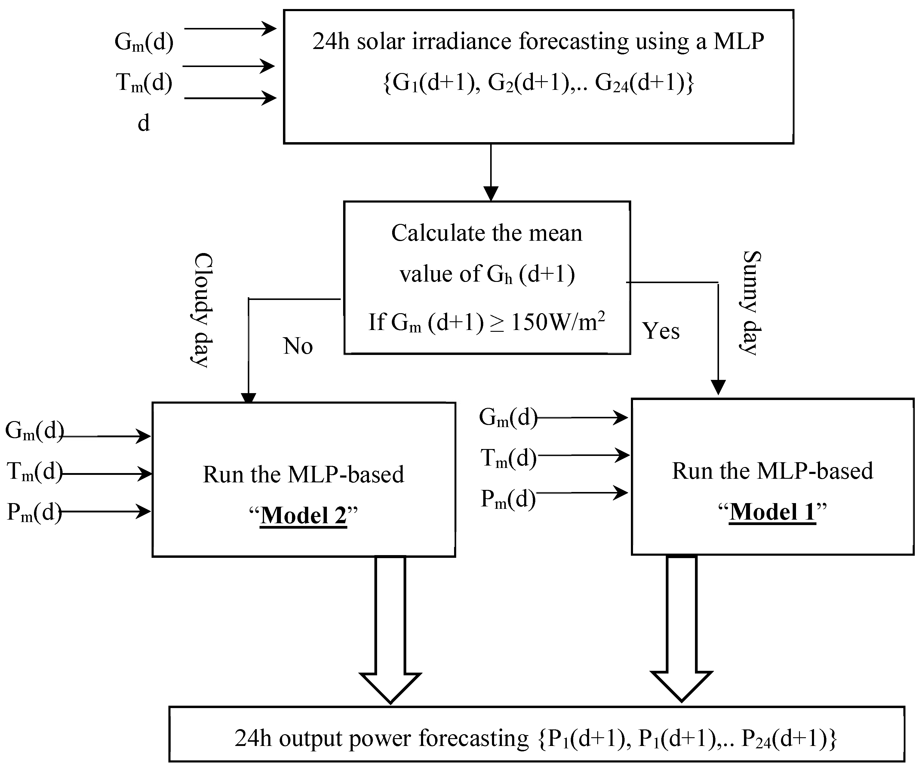
Three different MLPs have been developed to forecast the power produced by the PV plant. As shown in Figure 1, a first MLP-based forecaster is used to predict the solar irradiance of the next day. If the mean value of the forecasted irradiance is greater than 150 W/m2, a MLP called “model 1” is used to predict the produced power. This forecaster has been specifically developed using the dataset corresponding to the 154 “sunny days.” Otherwise, if the mean forecasted irradiance is smaller than 150 W/m2, the so-called “model 2,” which was developed using the part of the dataset corresponding to the 114 “cloudy days,” is used.
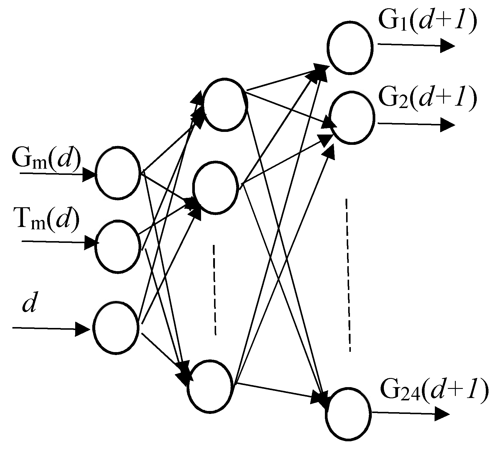
The input of the first MLP forecaster is the mean values of the solar irradiance Gm(d) and of the air temperature Tm(d) together with the number of the day d; the output can then be expressed as:
{ G 1 ( d + 1 ) ,   G 2 ( d + 1 ) , ,   G 24 ( d + 1 ) } = f G ( G m ( d ) ,   T m ( d ) , d ) ,
where fG is the approximate function, and G1 (d + 1), G2 (d + 2)… G24 (d + 1) are the hourly values of the forecasted solar irradiance. The structure of the MLP is sketched in Figure 2 and was developed using 240 days of the original dataset, while 28 days have been used for the testing of the network.
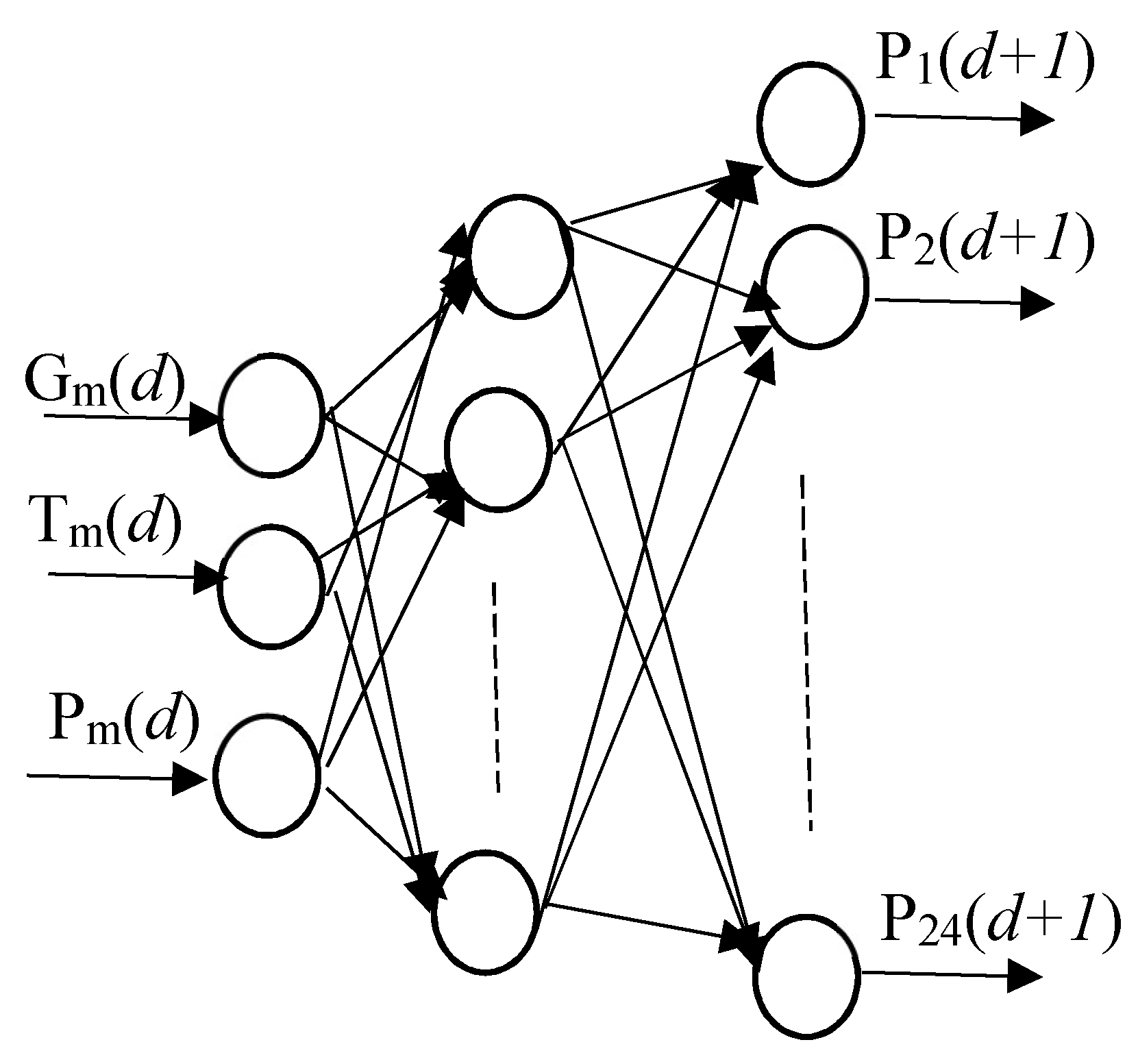
As shown in Figure 3, the input of the second and third MLPs is the mean values of the daily solar irradiance Gm(d) and of the air temperature Tm(d), together with the mean produced power Pm(d). The output layer has 24 output nodes corresponding to the produced hourly power of the next day {P1(d + 1), P1(d + 2),…, P1(d + 24)}.
The output of the neural network can then be expressed as:
{ P 1 ( d + 1 ) ,   P 2 ( d + 1 ) , ,   P 24 ( d + 1 ) } = f P ( G m ( d ) ,   T m ( d ) ,   P m ( d ) ) ,
where fP is an approximate function, and P1 (d + 1), P2 (d + 1) … P24 (d + 1) are the forecasted values of the hourly power. The MLP called model 1 as it is shown in Figure 4 has been developed using data for the 147 sunny days, while seven days have been used for the test. Model 2 has been built using 114 cloudy days, and also tested on seven days.
In both cases, the original data have been pre-processed as follows [53]:
y = y m i n + ( x x m i n ) ( x m a x x m i n ) 1 ( y m a x y m i n ) ,
where x ∈ [xmin xmax] and y ∈ [ymin ymax] are the original data and the corresponding normalized variable, respectively. ymin and ymax have been set to between {−1, 1}.
Case 2:
The implemented method to perform the simulations in this second case is still based on a FFNN but, among the inputs, the irradiation in clear sky conditions is provided. This method is called Physical Hybrid Artificial Neural Network (PHANN) and its model is shown in Figure 5. The Clear Sky Radiation Model (CSRM) adopted is described in [54] and was validated on measured data available from the SolarTechLab at the Politecnico di Milano. Since the result of a physical model is fed into the network, the artificial neural network is hybridized, as explained in [45]. The network’s architecture adopted here consists of two hidden layers, including 12 and five neurons, respectively. In order to train the network, 90% of the samples are randomly assigned to the training set, while the remaining 10% are assigned to the validation set. Furthermore, we decided to use 40 trials for the ensemble logic. These characteristics of the ANN have been set in a sensitivity analysis, which was performed in a previous work [55].
To properly evaluate how sensitive the forecast is to different training methodologies and database composition, several simulations were run. In particular, three approaches are adopted according to the cluster of the day to be forecast (i.e., “Sunny” or “Cloudy”):
  • Ap1: All the available data are used to train the network (268 days)
  • Ap2: The simulations are performed using the dataset comprising all the available data but, in order to train the network, the same number of days available in the sunny and cloudy dataset is used (randomly picked)
  • Ap3: The simulations are performed using the “Sunny” and “Cloudy” dataset alternatively.

4. Results and Discussion

Case 1
As result, Figure 6 shows a comparison between the measured and forecasted hourly output power of the PV plant for both sunny and cloudy days. With reference to the sunny days, it is clearly observed that the MLP-based model for sunny days shows good accuracy (MAPE% 23.6%). The second MLP-based model, which is designed for cloudy days, does not provide good results (54.0%).
Case 2
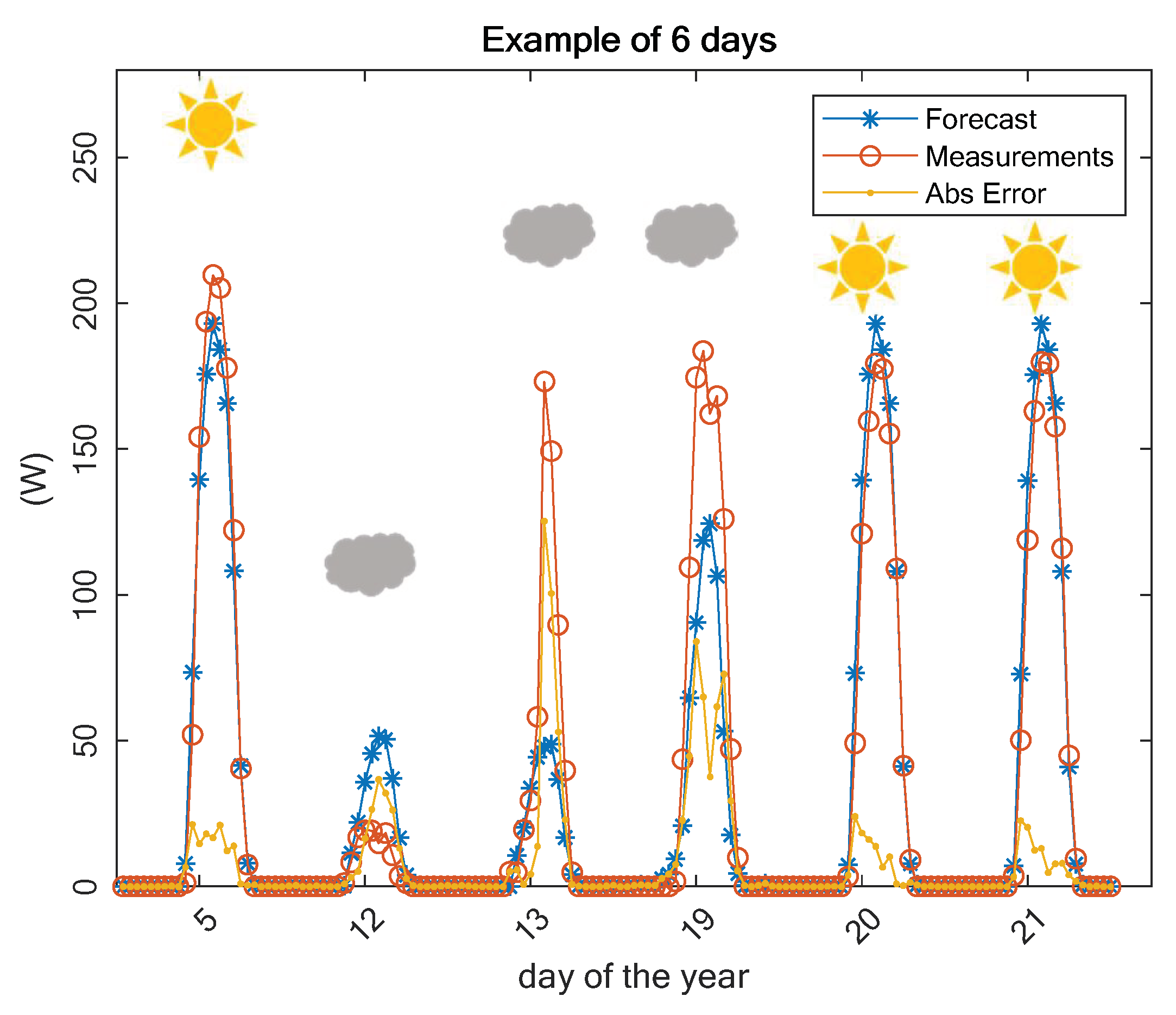
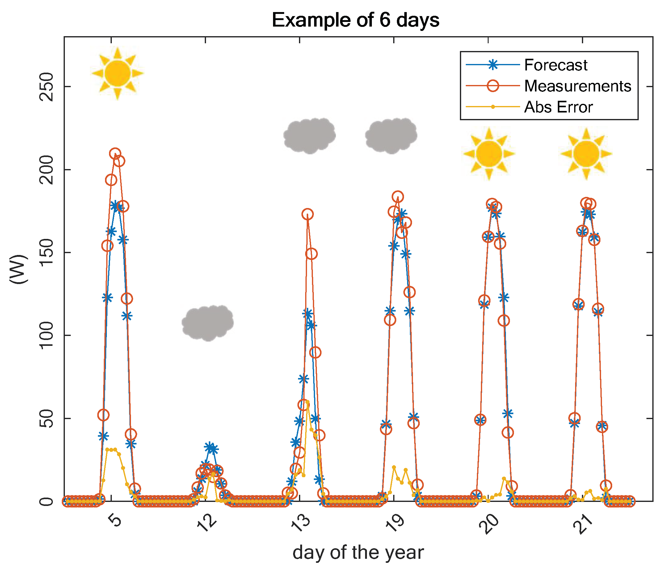
In Figure 7, the results referring to six available days, selected from the sunny and cloudy day datasets, are plotted. The blue line represents the power forecast provided by the NN for the PV module, the orange line the measurements, while the yellow line is the absolute error contributed by the implemented method. The method shows good forecasting performance, especially for sunny days, as during most of the hours the forecast and the measurements overlapped and the hourly absolute error was very low. As for the sunny days, the MAPE% was 10.0%, while for the cloudy days it was around 68.9%.
Comparison between the two cases
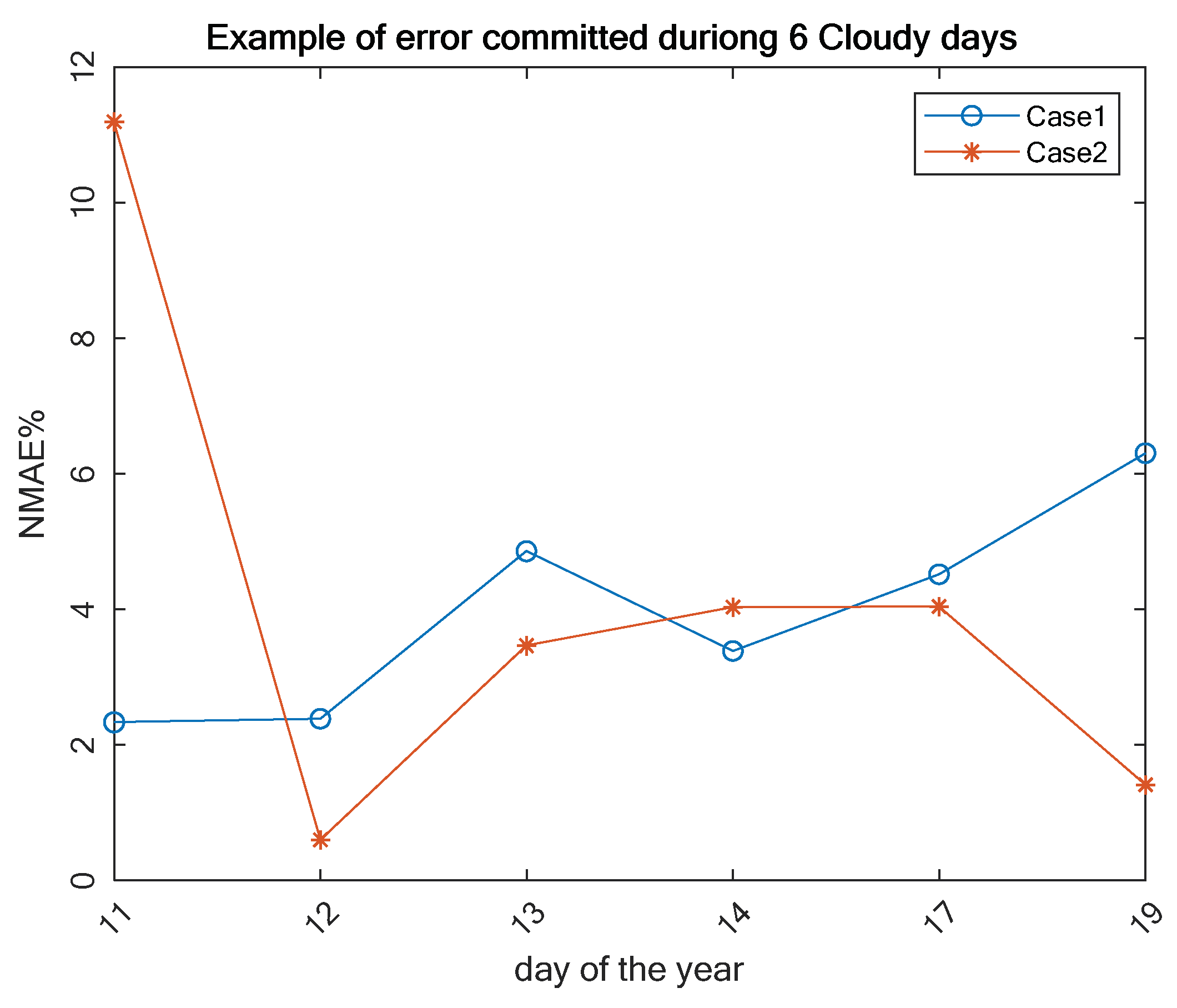
In Figure 8 and Figure 9, graphical representations of NMAE% error for the two cases are provided for the first six available sunny and cloudy days. In both graphs, the blue line represents the error observed for case 1, while the orange line represents the error observed for case 2, adopting the third approach. As can be noted, for sunny days the error given by model number 1 is quite stable and almost always lower than 2%, while in the second case the error shows a peak on the 16th day and is lower than the one from the first case for days 20 and 21. With reference to cloudy days, the two models performed similarly except for the 11th day, when the error from model 2 was larger than 11%.
The forecasting performance of the two models, for the same days presented in Figure 8 and Figure 9, is reported in terms of in Table 3 and Table 4. No clear evidence of an unequivocally better performing method can be observed. The mean WMAE% for sunny days is 10.1% and 12.4% for cases 1 and 2, respectively, while for the cloudy days the mean WMAE% is 78.1% and 151.0%, respectively.

5. Conclusions

Two of the most widely used and effective forecasting ANN-based methods for the performance of PV systems have been compared. Specifically, we analyzed the 24-h-ahead power forecasting performance of the two methods, as this is arguably one of the most important kinds of predictions for the energy generation, transmission, and distribution industry.
The dataset used in this study (collected at the SolarTechLab of the Politecnico of Milan, Italy) is a historical hourly series including the climatic parameters and the simultaneous electric parameters of the photovoltaic system.
One method feeds exclusively upon data from the dataset—in this case the solar irradiance and the ambient temperature. The other method uses a hybrid approach, including as an input the daily weather forecast. In both cases, the dataset has been clustered, identifying a group of sunny days and a group of cloudy days.
The comparison is self-consistent and homogeneous, as the dataset used for the network training and testing is the same for both methods, unlike the comparisons currently available in the literature. Also, in contrast to the available literature reviews, we used the same metrics for comparing the two methods. We also compared a wide range of metrics, demonstrating a high degree of correlation among them, and therefore there was the possibility, as a first approximation, of using a subset of metrics to assess the overall performance of a method.
The results show the good forecasting performance of both methods in the case of sunny days. While the hybrid method shows an excellent performance for some specific days (NMAE% < 1% in two cases; WMAE% < 4% in three cases), the second method under study shows a more stable and consistently good performance (NMAE consistently between 1% and 2%; WMAE% oscillating between 7% and 13%).
The forecasting performance of both methods drops significantly for cloudy days. Again, while the performance of the hybrid method is better for some specific days, for at least one day the prediction is rather poor (NMAE% > 11% and WMAE% = 750), and the method that feeds exclusively on data from the dataset shows more stable performance on both NMAE and WMAE metrics.
A possible explanation for the lower performance of both methods for cloudy days is the rather high relative variability of the irradiance conditions in this cluster, making the training of the network less reliable. In fact, cloudy days are identified as days where the average irradiation is less than 150 W/m2, so even a small variation translates to a large relative variation. Conversely, the irradiation in sunny days is always close to its maximum value (typically near 1000 W/m2) for the specific location; the variations are typically small, and even more so in relative terms. Training on this cluster is therefore expected to lead to more repeatable predictions.
As a possible explanation of the less stable performance of the hybrid model with respect to the model where the forecasts are not used, one can speculate that the forecasting ability of the first depends on the quality of the weather forecast for the specific day. Moreover, the quality of the forecast is strongly related to the location it refers to, which usually does not correspond exactly to the one where the PV system operates. A more detailed analysis considering this possible correlation is needed in order to verify this hypothesis.
This work shows that no one model outperforms the other under all possible conditions. Managers of utility-scale PV plants, manufacturers of power management systems, and distribution and transmission system operators can therefore benefit from the comparison presented in this work in order to identify the most suitable forecaster for the specific application at hand. Future work will investigate how to detect in advance the best forecasting method according to the different typology of the day, on the basis of the adopted classification (for, example by means of the clearness index or the mean values of the expected daily irradiation).

Author Contributions

conceptualization, E.O. and A.M.P.; methodology, E.O. and A.M.P.; software, A.M., A.N; validation, E.O. and A.M.P.; formal analysis, S.L. and V.L.; investigation, S.L.; resources, A.D.; data curation, A.N.; writing—original draft preparation, E.O. and A.M.P.; writing—review and editing, V.L.; visualization, A.D.; supervision, S.L.; project administration, E.O. and A.M.P.; funding acquisition, E.O. and A.M.P.

Funding

This research received no external funding.

Conflicts of Interest

The authors declare no conflict of interest.

References

  1. Executive Summary of the World Energy Investment, 2018. International Energy Agency, 2018. Available online: https://webstore.iea.org/world-energy-investment-2018 (accessed on 22 March 2019).
  2. Global Warming of 1.5. 2018. Special Report IPCC, 2018. Available online: https://www.ipcc.ch/sr15/ (accessed on 22 March 2019).
  3. Zhan, D.; Kwan, M.P.; Zhang, W.; Yu, X.; Meng, B.; Liu, Q. The driving factors of air quality index in China. J. Clean. Prod. 2018, 197, 1342–1351. [Google Scholar] [CrossRef]
  4. Ul’Yanin, Y.A.; Kharitonov, V.V.; Yurshina, D.Y. Forecasting the Dynamics of the Depletion of Conventional Energy Resources. Stud. Russ. Econ. Dev. 2018, 29, 153–160. [Google Scholar] [CrossRef]
  5. Massi Pavan, A.; Lughi, V.; Rosato, P.; Spertino, F.; Vergura, S. Diminishing cost of electricity from wind power and photovoltaics. In Proceedings of the 2017 IEEE International Conference on Environment and Electrical Engineering and 2017 IEEE Industrial and Commercial Power Systems Europe (EEEIC/I&CPS Europe), Milan, Italy, 6–9 June 2017. [Google Scholar]
  6. Global landscape of Renewable Energy Finance. IRENA, 2018. Available online: https://www.irena.org/publications/2018/Jan/Global-Landscape-of-Renewable-Energy-Finance (accessed on 22 March 2019).
  7. D’Alessandro, V.; Di Napoli, F.; Guerriero, P.; Daliento, S. An automated high-granularity tool for a fast evaluation of the yield of PV plants accounting for shading effects. Renew. Energy 2015, 83, 294–304. [Google Scholar] [CrossRef]
  8. Massi Pavan, A.; Lughi, V. Grid parity in the Italian commercial and industrial electricity market. In Proceedings of the 2013 IEEE 4th International Conference on Clean Electrical Power (ICCEP), Alghero, Italy, 11–13 June 2013. [Google Scholar]
  9. Massi Pavan, A.; Lughi, V. Photovoltaics in Italy: Toward grid parity in the residential electricity market. In Proceedings of the 2012 24th International Conference on Microelectronics (ICM), Algiers, Algeria, 16–20 December 2012. [Google Scholar]
  10. Daliento, S.; Aissa, C.; Guerriero, P.; Massi Pavan, A.; Mellit, A.; Moeini, R.; Tricoli, P. Monitoring, diagnosis, and power forecasting for photovoltaic fields: A review. Int. J. Photoenergy 2017, 2017, 1–13. [Google Scholar] [CrossRef]
  11. Massi Pavan, A.; Sulligoi, G.; Lughi, V.; Pauli, F.; Miceli, R.; Di Dio, V.; Viola, F. Leading the way toward fuel parity in photovoltaics: The utility-scale market in Sicily, Italy. In Proceedings of the 2016 IEEE 16th International Conference on Environment and Electrical Engineering (EEEIC), Florence, Italy, 7–10 June 2016. [Google Scholar]
  12. Dolara, A.; Leva, S.; Mussetta, M.; Ogliari, E. PV hourly day-ahead power forecasting in a micro grid context. In Proceedings of the 2016 IEEE 16th International Conference on Environment and Electrical Engineering (EEEIC), Florence, Italy, 7–10 June 2016. [Google Scholar]
  13. Bird, L.; Cochran, J.; Wang, X. Wind and Solar Energy Curtailment: Experience and Practices in the United States; Technical Report NREL/TP-6A20-60983; National Renewable Energy Laboratory: Golden, CO, USA, March 2014. [Google Scholar]
  14. Sobri, S.; Koohi-Kamali, S.; Rahim, N.A. Solar photovoltaic generation forecasting methods: A review. Energy Convers. Manag. 2018, 156, 459–497. [Google Scholar] [CrossRef]
  15. De Giorgi, M.G.; Malvoni, M.; Congedo, P.M. Photovoltaic power forecasting using statistical methods: Impact of weather data. IET Sci. Meas. Technol. 2014, 8, 90–97. [Google Scholar] [CrossRef]
  16. Raza, M.Q.; Nadarajah, M.; Ekanayake, C. On recent advances in PV output power forecast. Sol. Energy 2016, 136, 125–144. [Google Scholar] [CrossRef]
  17. Connecting the Sun-Solar Photovoltaics on the Road To Large Scale Grid Integration. EPIA, 2012. Available online: http://pvtrin.eu/assets/media/PDF/Publications/other_publications/263.pdf (accessed on 22 March 2019).
  18. Antonanzas, J.; Osorio, N.; Escobar, R.; Urraca, R.; Martinez-De-Pison, F.; Antonanzas-Torres, F. Review of photovoltaic power forecasting. Sol. Energy 2016, 136, 78–111. [Google Scholar] [CrossRef]
  19. Mills, A.; Wiser, R. Implications of Wide-Area Geographic Diversity for Short-Term Variability of Solar Power; Technical Report LBNL-3884E; Lawrence Berkeley National Laboratory: Washington, DC, USA, September 2010. [Google Scholar]
  20. Mills, A.; Botterud, A.; Wu, J.; Zhou, Z.; Hodge, B.M.; Heaney, M. Integrating Solar PV in Utility System Operation; Report ANL/DIS-13/18; Argonne National Laboratory: Lemont, IL, USA, October 2013. [Google Scholar]
  21. Montgomery, D.C.; Jennings, C.L.; Kulahci, M. Introduction to Time Series Analysis and Forecasting, 1st ed.; Wiley: Hoboken, NJ, USA, 2008. [Google Scholar]
  22. Mellit, A.; Massi Pavan, A. A 24-h forecast of solar irradiance using artificial neural network: Application for performance prediction of a grid-connected {PV} plant at Trieste, Italy. Sol. Energy 2010, 84, 807–821. [Google Scholar] [CrossRef]
  23. Mellit, A.; Shaari, S. Recurrent neural network-based forecasting of the daily electricity generation of a photovoltaic power system. Ecolog. Veh. Renew. Energy 2009, 2–7. [Google Scholar]
  24. Mellit, A.; Saǧlam, S.; Kalogirou, S.A. Artificial neural network-based model for estimating the produced power ofaphotovoltaic module. Renew. Energy 2013, 60, 71–78. [Google Scholar] [CrossRef]
  25. Mellit, A.; Massi Pavan, A.; Benghanem, M. Least squares support vector machine for short-term prediction of meteorological time series. Theor. Appl. Climatol. 2013, 111, 297–307. [Google Scholar] [CrossRef]
  26. Reikard, G. Predicting solar radiation at high resolutions: A comparison of time series forecasts. Sol. Energy 2009, 83, 342–349. [Google Scholar] [CrossRef]
  27. Mellit, A.; Massi Pavan, A.; Lughi, V. Short-term forecasting of power production in a large-scale photovoltaic plant. Sol. Energy 2014, 105, 401–413. [Google Scholar] [CrossRef]
  28. Shi, J.; Lee, W.J.; Liu, Y.; Yang, Y.; Wang, P. Forecasting power output of photovoltaic systems based on weather classification and support vector machines. IEEE Trans. Ind. Appl. 2012, 48, 1064–1069. [Google Scholar] [CrossRef]
  29. Yang, C.; Thatte, A.A.; Xie, L. Multitime-scale data-driven spatio-temporal forecast of photovoltaic generation. IEEE Trans. Sustain. Energy 2015, 6, 104–112. [Google Scholar] [CrossRef]
  30. Yang, H.-T.; Chao-Ming, H.; Huang, Y.-C.; Yi-Shiang, P. A Weather-Based Hybrid Method for one-day Ahead Hourly Forecasting of PV Power Output. IEEE Trans. Sustain. Energy 2014, 5, 917–926. [Google Scholar]
  31. Chen, C.; Duan, S.; Cai, T.; Liu, B. Online 24-h solar power forecasting based on weather type classification using artificial neural network. Sol. Energy 2011, 85, 2856–2870. [Google Scholar] [CrossRef]
  32. Yona, A.; Senjyu, T.; Funabashi, T.; Kim, C.H. Determination method of insolation prediction with fuzzy and applying neural network for long-term ahead PV power output correction. IEEE Trans. Sustain. Energy 2013, 4, 527–533. [Google Scholar] [CrossRef]
  33. Hoff, T.E.; Perez, R.; Kleissl, J.; Renne, D.; Stein, J. Reporting of irradiance modeling relative prediction errors. Prog. Photovoltaics Res. Appl. 2016, 9, 261–270. [Google Scholar] [CrossRef]
  34. Pelland, S.; Galanis, G.; Kallos, G. Solar and photovoltaic forecasting through post-processing of the Global Environmental Multiscale numerical weather prediction model. Prog. Photovoltaics Res. Appl. 2011, 9, 261–270. [Google Scholar] [CrossRef]
  35. Monteiro, C.; Fernandez-Jimenez, L.A.; Ramirez-Rosado, I.J.; Muñoz-Jimenez, A.; Lara-Santillan, P.M. Short-term forecasting models for photovoltaic plants: Analytical versus soft-computing techniques. Math. Probl. Eng. 2013, 2013. [Google Scholar] [CrossRef]
  36. Das, U.K.; Tey, K.S.; Seyedmahmoudian, M.; Mekhilef, S.; Idris, M.Y.I.; Deventer, W.V.; Horan, B.; Stojcevski, A. Forecasting of photovoltaic power generation and model optimization: A review. Renew. Sustain. Energy Rev. 2018, 81, 912–928. [Google Scholar] [CrossRef]
  37. Monteiro, C.; Santos, T.; Fernandez-Jimenez, L.A.; Ramirez-Rosado, I.J.; Terreros-Olarte, M.S. Short-term power forecasting model for photovoltaic plants based on historical similarity. Energies 2013, 6, 2624–2643. [Google Scholar] [CrossRef]
  38. Diagne, M.; David, M.; Lauret, P.; Boland, J.; Schmutz, N. Review of solar irradiance forecasting methods and a proposition for small-scale insular grids. Renew. Sustain. Energy Rev. 2013, 27, 65–76. [Google Scholar] [CrossRef]
  39. Soman, S.S.; Zareipour, H.; Malik, O.; Mandal, P. A review of wind power and wind speed forecasting methods with different time horizons. In Proceedings of the North American Power Symposium 2010, Arlington, TX, USA, 26–28 September 2010; pp. 1–8. [Google Scholar]
  40. Leva, S.; Dolara, A.; Grimaccia, F.; Mussetta, M.; Ogliari, E. Analysis and validation of 24 hours ahead neural network forecasting of photovoltaic output power. Math. Comput. Simul. 2017, 131, 88–100. [Google Scholar] [CrossRef] [Green Version]
  41. Mandal, P.; Madhira, S.T.S.; Ul haque, A.; Meng, J.; Pineda, R.L. Forecasting power output of solar photovoltaic system using wavelet transform and artificial intelligence techniques. Procedia Comput. Sci. 2012, 12, 332–337. [Google Scholar] [CrossRef]
  42. Gensler, A.; Henze, J.; Sick, B.; Raabe, N. Deep Learning for solar power forecasting—An approach using AutoEncoder and LSTM Neural Networks. In Proceedings of the 2016 IEEE International Conference on Systems, Man, and Cybernetics (SMC), Budapest, Hungary, 9–12 October 2016. [Google Scholar]
  43. Omar, M.; Dolara, A.; Magistrati, G.; Mussetta, M.; Ogliari, E.; Viola, F. Day-ahead forecasting for photovoltaic power using artificial neural networks ensembles. In Proceedings of the 2016 IEEE International Conference on Renewable Energy Research and Applications (ICRERA), Birmingham, UK, 20–23 November 2016; pp. 1152–1157. [Google Scholar]
  44. Fernandez-Jimenez, L.A.; Muñoz-Jimenez, A.; Falces, A.; Mendoza-Villena, M.; Garcia-Garrido, E.; Lara-Santillan, P.M.; Zorzano-Alba, E.; Zorzano-Santamaria, P.J. Short-term power forecasting system for photovoltaic plants. Renew. Energy 2012, 44, 311–317. [Google Scholar] [CrossRef]
  45. Dolara, A.; Grimaccia, F.; Leva, S.; Mussetta, M.; Ogliari, E. A physical hybrid artificial neural network for short term forecasting of PV plant power output. Energies 2015, 8, 1138–1153. [Google Scholar] [CrossRef]
  46. Bouzerdoum, M.; Mellit, A.; Massi Pavan, A. A hybrid model (SARIMA-SVM) for short-term power forecasting of a small-scale grid-connected photovoltaic plant. Sol. Energy 2013, 98, 226–235. [Google Scholar] [CrossRef]
  47. Chicco, G.; Cocina, V.; Di Leo, P.; Spertino, F.; Massi Pavan, A. Error assessment of solar irradiance forecasts and AC power from energy conversion model in grid-Connected photovoltaic systems. Energies 2016, 9, 8. [Google Scholar] [CrossRef]
  48. Lee, D.; Kim, K. Recurrent Neural Network-Based Hourly Prediction of Photovoltaic Power Output Using Meteorological Information. Energies 2019, 12, 215. [Google Scholar] [CrossRef]
  49. SolarTech LAB. 2013. Available online: http://www.solartech.polimi.it/ (accessed on 20 April 2019).
  50. Ulbricht, R.; Fischer, U.; Lehner, W.; Donker, H. First Steps Towards a Systematical Optimized Strategy for Solar Energy Supply Forecasting. ECML/PKDD 2013, 1st Int. Work. Data Anal. Renew. Energy Integr. 2013, 2327, 14–25. [Google Scholar]
  51. Coimbra, R.; Carlos, F.M.; Kleissl, J.; Marquez, R. Overview of Solar-Forecasting Methods and a Metric for Accurary Evaluation. In Solar Energy Forecasting and Resource Assessment; Academic Press: Cambridge, MA, USA, 2013; pp. 171–193. Available online: https://www.sciencedirect.com/science/article/pii/B9780123971777000085?via%3Dihub (accessed on 20 April 2019).
  52. Leva, S.; Mussetta, M.; Ogliari, E. PV module fault diagnosis based on micro-converters and day-ahead forecast. IEEE Trans. Ind. Electron. 2018, 66, 3928–3937. [Google Scholar] [CrossRef]
  53. Mellit, A.; Kalogirou, S.A. Artificial intelligence techniques for photovoltaic applications: A review. Prog. Energy Combust. Sci. 2008, 34, 574–632. [Google Scholar] [CrossRef]
  54. Bird, R.E.; Riordan, C. Simple Solar Spectral Model for Direct and Diffuse Irradiance on Horizontal and Tilted Planes at the Earth’s Surface for Cloudless Atmospheres. 1986. Available online: https://journals.ametsoc.org/doi/pdf/10.1175/1520-0450%281986%29025%3C0087%3ASSSMFD%3E2.0.CO%3B2 (accessed on 20 April 2019).
  55. Grimaccia, F.; Leva, S.; Mussetta, M.; Ogliari, E. ANN sizing procedure for the day-ahead output power forecast of a PV plant. Appl. Sci. 2017, 7, 622. [Google Scholar] [CrossRef]
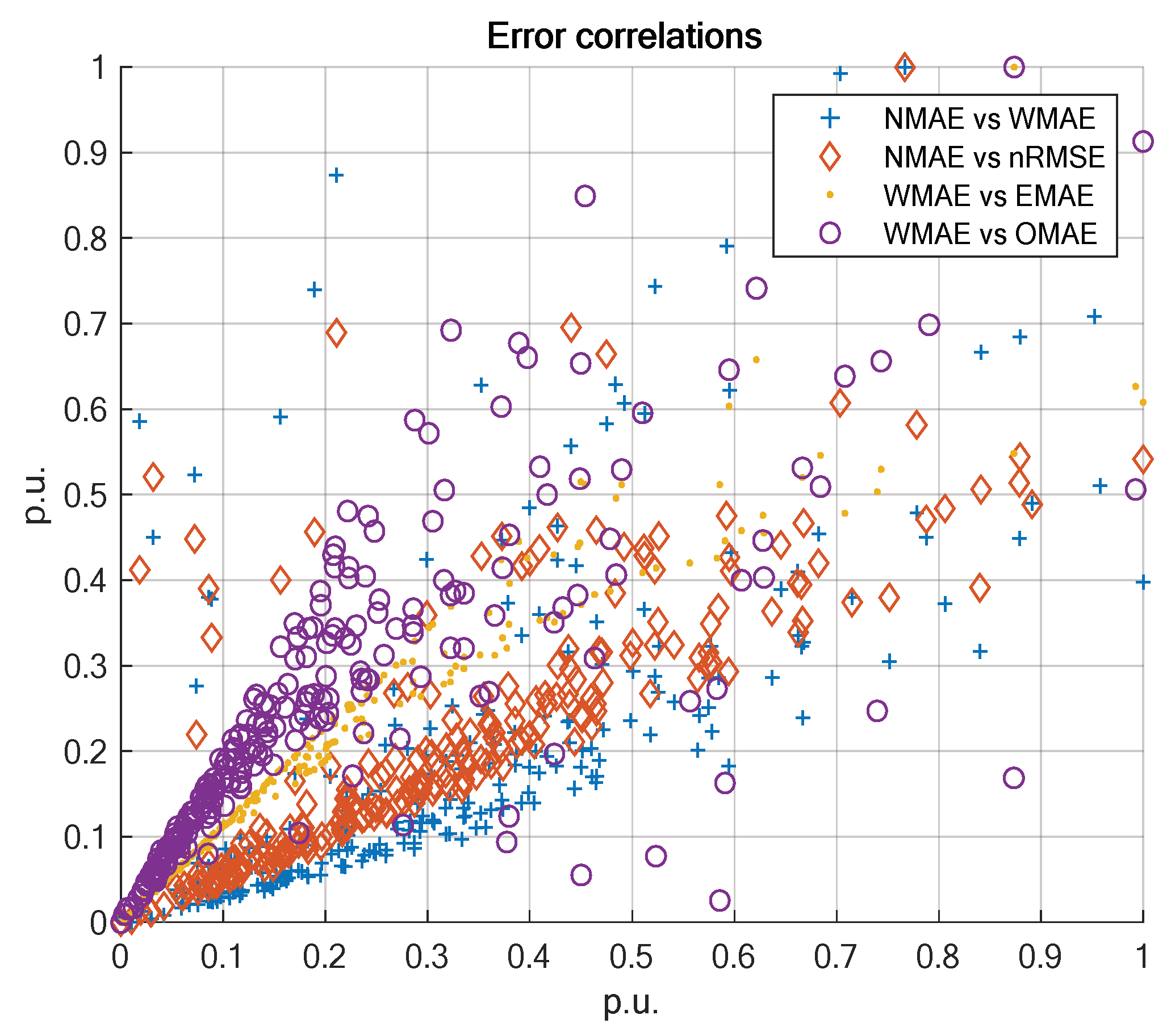
Figure 1. Scatterplot of the error correlations.
Energies 12 01621 g001
Figure 2. Block diagram of the proposed procedure.
Energies 12 01621 g002
Figure 3. Block diagram of the proposed procedure.
Energies 12 01621 g003
Figure 4. MLP used for the power forecasting.
Energies 12 01621 g004
Figure 5. PHANN method.
Energies 12 01621 g005
Figure 6. Measured vs. forecasted output power by MLP (sunny days and cloudy days).
Energies 12 01621 g006
Figure 7. Example of measured and forecast DC power output together with the absolute error for some sample days of the sunny dataset.
Energies 12 01621 g007
Figure 8. Example of six sunny days.
Energies 12 01621 g008
Figure 9. Example of six cloudy days.
Energies 12 01621 g009
Table 1. Error correlation coefficients.
NMAEEMAEWMAEnRMSEOMAE
NMAE10.590.370.400.90
EMAE 10.800.780.71
WMAE 10.980.48
nRMSE 10.51
OMAE 1
Table 2. Available datasets.
Imposed Threshold on GPOA,f,d150 (W/m2)
# of days268
# of sunny days154
# of cloudy days114
Table 3. WMAE% comparison of sunny days.
SunnyDay 5Day 15Day 16Day 18Day 20Day 21
Case 110.8312.8910.457.179.519.61
Case 214.9521.4330.391.962.223.29
Table 4. WMAE% comparison of cloudy days.
CloudyDay 11Day 12Day 13Day 14Day 17Day 19
Case 1156.21143.1557.8626.5142.6342.01
Case 2750.0135.8741.2631.638.149.38