Abstract
Bypassing transient current through copper (Cu) stabilizer layers reduces heat generation and temperature rise of high-temperature superconducting (HTS) conductors, which could protect HTS cables from burning out during transient conditions. The Cu layer connected in parallel with HTS tape layers impacts current distribution among layers and variations of phase resistance in either steady-state or transient conditions. Modeling the multilayer HTS power cable is important for transient studies. However, existing models of HTS power cables have only proposed HTS cables without the use of a Cu-former layer. To overcome this problem, the authors proposed a multilayer HTS power cable model that used a Cu-former layer in each phase for transient study. It was observed that resistance of the HTS conductor increased significantly in the transient state due to a quenching phenomenon, which made the transient current mainly flow into the Cu-former layers. Since resistance of the Cu-former layer has a significant impact on the transient current, detailed modeling of the Cu-former layer is described in this study. The feasibility of the developed HTS cable model is evaluated in the PSCAD/EMTDC program.
1. Introduction
High-temperature superconducting (HTS) power cables are suitable for high-load areas such as dense urban districts of large cities, where construction of additional substations could be cost-prohibitive [1,2,3,4]. HTS power cables could transfer a considerable amount of power compared to traditional low-capacity cables. In addition, in dense urban areas, substations could reach capacity limits and require redundant transformer capacities to improve system reliability. HTS cables could tie these existing stations to improve grid power transmission and avoid upgrading costly transformers and construction costs [5].
Various configuration of HTS power cables have been reported, such as single-core cable, triaxial cable, and coaxial cable [4]. Among these configurations, coaxial HTS cables have been studied widely recently, since this configuration can reduce AC loss by designing proper parameters such as radius, direction, and twisting pitch [6,7]. Multiple layers of HTS tapes are used to enhance cable capacity. Unlike traditional power cables, resistance and temperature of HTS power cables are significantly varied by fault current, which leads to an increase in a large amount of thermal energy [8]. In severe conditions, HTS cables could be damaged or degraded [9]. Thus, HTS tape layers are connected in parallel with the Cu-former layer to reduce heat generation and temperature rise during fault conditions. A part of the large fault current flows into the Cu-former layers, which could protect the HTS conductor from burning out [10,11,12,13].
Modeling the HTS power cable plays an important role in improving cable design and performance. Numerical models, which are able to simulate electromagnetic and thermal behaviors [14], have become indispensable in predicting cable performance and improving their design. Either finite element analysis (FEA) or finite-difference time-domain (FDTD) analysis of numerical models provides a valuable resource, as they remove multiple instances of creation and testing of hard prototypes for various high-fidelity situations. Various tools based on FEA and FDTD could be used for numerical models of HTS cables, such as MATLAB [15,16], ANSYS [17,18], COMSOL [19,20], etc. For time-dependent simulations such as fault analyses in the power system with HTS cables, the main limitation of numerical models based on FEM or FDTD is the computational burden. A simplified model of HTS cables should be developed for such analysis in power system studies.
Various simplified, time-dependent models of HTS cables have been proposed recently. Since analysis of AC loss in the steady-state condition is essential, an HTS cable model for steady-state analysis was proposed in [21], in which the resistance of this HTS cable in the steady-state condition was calculated based on an additional experimental measurement. Variation of HTS cable resistance during the transient condition could have negative impacts on the design of the protection system [22]. Thus, modelling the HTS power cable plays an important role in evaluating the HTS cable’s impact on the protection system. Various models of HTSs cable have been proposed recently. In [23], modelling of an HTS power cable in power system computer-aided design/electromagnetic transients including direct current (PSCAD/EMTDC) was presented. This HTS cable model was developed based on cable models from the master library. The quench phenomenon was simulated by a variable resistor that was connected in series with the library cable model. The advantage of using the library model is its ability to model current distribution and surge effect of cable layers. The maximum layer number in the library model was eight, which was one of the limitations of this model. Real HTS cables should be simplified as an equivalent cable with eight layers if the number of real HTS layers exceeds eight. Simplified HTS cable models, which only simulate the conducting and shield layers, were proposed in [24,25,26,27,28]. The quench phenomenon was modeled by variable resistors while current distribution of the HTS cable was simulated by self and mutual inductance based on the transformer section in the PSCAD/EMTDC program. Internal temperature change of each layer was also modeled to evaluate the impact of temperature on the resistance of the HTS cable. However, in the case of the multilayer HTS cable, these models are complicated because the temperature of each layer needs to be modeled individually. In addition, impact of the Cu-former on current distribution of each layer was not considered in these models.
Although various HTS cable models have been presented recently, modeling of HTS cables with Cu-former layers has not been studied. In multilayer HTS power cables, each phase could consist of multiple layers, including the Cu-former layer. The equivalent impedance of each phase is dependent on current distribution among layers. Thus, modeling HTS power cables considering the effect of the Cu-former layer is important for the transient study. Existing approaches to model multilayer HTS power cables are complicated. Thus, this study proposes a straightforward approach to model a multilayer HTS power cable with Cu-former layers in each phase. The temperature rise of the HTS cable causes increases in the resistance of the HTS tape and Cu-former layers. Since resistance of the HTS tape layer increases significantly during the transient state because of the quench phenomenon, the fault current mainly flows into the Cu-former layer. The dramatic change in resistance of the HTS tape layer results in the change in equivalent resistance of each phase, which has a significant impact on fault current. Based on this observation, a simplified model of a multilayer HTS power cable is developed for the transient study. The feasibility of the developed cable model is evaluated in the PSCAD/EMTDC program.
The rest of this study is organized as follows. Section 2 describes the modeling of the coaxial, multilayer HTS power cable with the Cu-former layer in the PSCAD/EMTDC program. The tested system and simulation results are provided in Section 3. Finally, the main conclusions of this paper are summarized in Section 4.
2. Cable Modeling in PSCAD/EMTDC
Figure 1 shows the configuration of coaxial, multilayer HTS power cables that are used in domestic, distribution-grade superconducting cables to connect substations in Korea, in which the conventional 154 kV transmission system would be replaced by the 22.9 kV HTS cable system with the same transmission capacity [4]. Selection of the number of HTS tapes and layers was based on its designed critical current. The number of HTS tapes that can be arranged on the circumference of former A was limited. Thus, there were two HTS layers in phase A to sustain the required critical current. The Cu-former layer was placed with the HTS layer to protect the cable from burning out by bypassing the fault current. In addition, the former layer located at the innermost side of the HTS cable was for maintaining the shape of the HTS layer wound on the former. A shield stabilizer layer wound with copper tape was placed on the outside. Generally, polypropylene laminated paper (PPLP) is used between the conductive layer of each phase and the shield layer to form an insulating layer that has a thickness suitable for voltage specification. However, the effect of insulator layers on temperature is neglected, as its thermal response is much slower because there is a much higher thermal resistivity compared to copper.
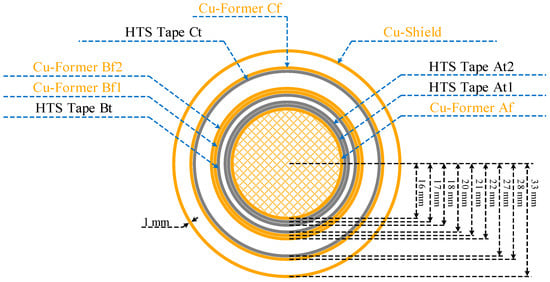
Figure 1.
Configuration of the coaxial, multilayer high-temperature superconducting (HTS) power cable; phase A consists of two HTS layers and one Cu-former layer; phase B consists of two Cu-former layers and one HTS layer; and phase C consists of one HTS layer and one Cu-former layer. The shield layer is based on copper.
Since the HTS cable in this study consisted of HTS layers and Cu-former layers in each phase, characteristics of the HTS cable were different regarding operation conditions. In normal conditions, the main current flowed through the HTS layers because the impedance of the HTS layer was much smaller than that of the Cu-former layer. However, in transient conditions, the fault current increased significantly, which resulted in the rapid increase of impedance of the HTS layer. Increased impedance of the superconducting cable due to the quenching phenomenon was much larger than the impedance of the Cu-former layer. Thus, the transient current mainly flowed through the Cu-former layers. Figure 2 shows the operation characteristics of the HTS cable in normal and transient conditions.
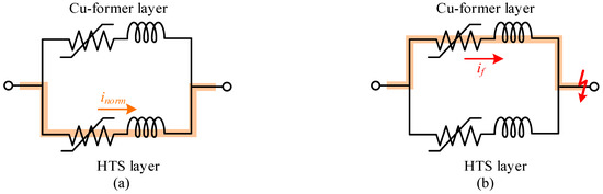
Figure 2.
Operation characteristics of the HTS cable: (a) current flow into each phase in the normal state; and (b) current flow into each phase in the transient state.
It was important to achieve uniform current distributions of each layer for the AC loss reduction of the HTS cable. Thus, the cable twist pitches should be optimally designed for each layer. Figure 3 shows the equivalent circuit of the multilayer HTS power cable. The mathematical model of the equivalent circuit is given by (1), in which the ground return impedance could be neglected in coaxial cable models [29].
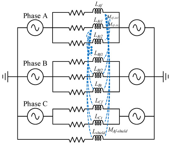
Figure 3.
The equivalent circuit of the HTS power cable.
The self and the mutual inductance of the HTS cable were dependent on the pitch length and radius of each layer, given by Equations (6) and (7).
where and are the radius of the each layer; is the permeability coefficient of the vacuum; and are the winding pitches of each layer; and are the winding direction of each layer (1 for clockwise and −1 for the counter-clockwise); and is the current return path. Equations (1)–(7) are used to calculate the resistance, inductance, and mutual inductance of each layer in the HTS cable. Then, these values would be used in the time-domain simulation based on the PSCAD/EMTDC program.
The resistance of each phase in the coaxial multilayer HTS cable was dependent on the HTS tape and Cu-former layers. In normal conditions, resistance of the HTS tape layer was nearly zero, while resistance of the Cu-former was relatively high compared to the HTS tape. However, in transient conditions, resistance of the HTS tape layer increased significantly due to a quench phenomenon. The rise in temperature caused an increase in cable resistance. The flowchart of the cable resistance calculations is shown in Figure 4a. The RMS current of each phase was measured firstly. If the RMS current was smaller than the critical current, the resistance of the HTS layer (RHTS) and the Cu-former (RCu) layer were equal to the resistance in the normal state. Otherwise, the resistance of the HTS layer was set to the maximal value that was obtained from experimental measurements, while the resistance of the Cu-former layer was calculated by the subprocess in Figure 4b. The process in Figure 4 was executed in every time-step. The rapid rise in the former current caused a change in energy dissipation (), resulting in an increased temperature (). The resistively of the former () was changed according to the increase of the temperature, which led to an increase in former resistance ().
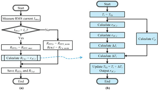
Figure 4.
Calculation of the resistance and temperature of the Cu-former layer i in each simulation step: (a) calculation process of the proposed model; and (b) subprocess calculates .
Resistance of the Cu-former layer was dependent on its geometric structure and temperature. Resistivity of the Cu-former i () was calculated by a linear form in (8), in which the temperature varied from 40 to 300 K. DC resistance of the Cu-former layer () was calculated based on the resistivity , as given by (9).
where Ti is the temperature of layer i in Kelvin; is the former effective area; l is the cable length in meters; and is in Ωm.
Since the former of phase A was different from the formers of phases B and C, the former effective area in phase A () was calculated by (10), whereas those of phases B and C were given by (11).
where is the radius of the Cu-former layer in phase A; k is the fill factor that describes the relationship between the electrical conducting cross-section to its total cross-sectional area; is the radius of the former phases B and C; and is the thickness of the former layer.
Skin depth () was proportional to the square root of the resistivity, as given by (12). It was assumed that the diameter of the former layer () was much thicker than , and the AC resistance of the former layer () could be solved by (13) [30].
where is the relative permeability of copper; is the permeability of free space; and f is the system frequency.
The energy dissipation () from the former layer was calculated based on AC resistance and the conducted current, as given by (14).
where is the measured current of the former layer and is the sampling time.
The volumetric heat capacity of the Cu-former layer () was based on the eighth-order interpolating polynomial in [31] and the copper density , as given by (16).
where is the density of copper in kg/m3; is the atomic mass of copper; volumetric heat capacity is in J/(Km3); and the coefficients are given by Table 1.

Table 1.
Coefficients of the copper heat capacity.
Temperature of the Cu-former layer varied slightly between 70 to less than 150 K. Thus, Equation (15) could be fitted as a quadratic form, as given by (16). Figure 5 shows the compared results of the volumetric heat capacity between the uses of the Equations (15) and (16). The quadratic form in (16) could be used to calculate the volumetric heat capacity of the former layer for the range of temperature between 40 and 140 K.
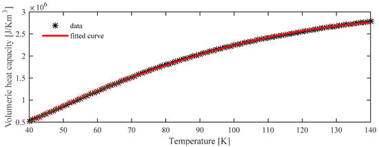
Figure 5.
Compared results between the uses of the eighth-order interpolating polynomial and quadratic form.
Finally, the temperature increment was calculated based on the specific heat capacity, energy dissipation , and the former volume , as given by (17).
where .
AC resistance of the former layer was saved in each iteration and used for modeling the HTS cable in the transient state. The model of the coaxial multilayer HTS power cable in PSCAD/EMTDC is shown in Figure 6. Resistances of the HTS cable were modeled by the variable RLC component. With the use of a custom model design, the flowchart to calculate the cable resistance shown in Figure 4 was implemented in FORTRAN language. The self and mutual inductances of the HTS cable were also implemented by a custom model in PSCAD/EMTDC with the use of a transformer section.
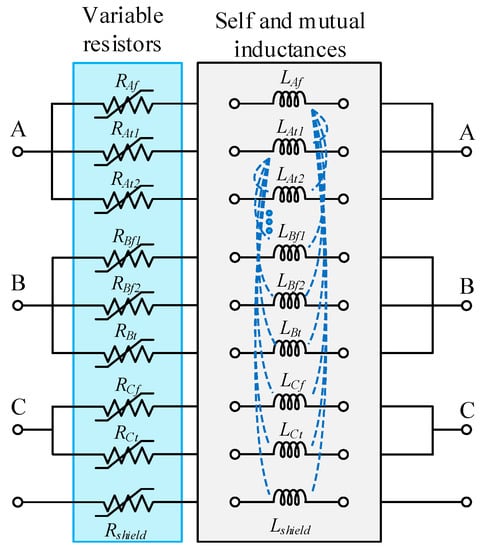
Figure 6.
Cable modeling in PSCAD/EMTDC.
3. Simulation Results
3.1. Validation of the High-Temperature Superconducting (HTS) Cable Model
Temperature variations of the Cu-former layer are discussed in this section. A comparison of the experiment and simulation of the Cu-former temperature was shown to validate the principle of the simplified HTS power cable model. The experimental results of the HTS cable with the Cu-former temperature were given in [32]. A model of a single-phase HTS cable with the Cu-former layer, which is shown in Figure 7, was simulated to show temperature variation. The radius of the Cu-former layer was 9.6 mm while that of the HTS tape layer was 10 mm. Gifford-McMahon cryocoolers were used to cool down the HTS cable by regulating the flow rate of the subcooled nitrogen. Power supply with a maximum current of 15 kA and voltage measurement through the National Instruments SCXI-1125 were used for the experiment. More details on the experiment could be found in [32].
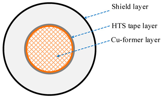
Figure 7.
Single-phase HTS power cable.
The compared results of temperature variation between the simulation model and the experimental measurements are shown in Figure 8. The cable was tested by different values of the RMS current, such as 14.9 and 9.9 kA. It was shown that the temperature of the Cu-former layer increased with the conducting current and the conducting time. Initially, the cable temperature was 77 K. The temperature of the Cu-former layer increased to 86 K when a current of 14.9 kA flowed into the cable for 1 s. Similar results of the temperature variation between simulation and experiment are observed in Figure 8. Thus, the principle of the simplified model could be extended to a multilayer HTS power cable.
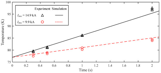
Figure 8.
Comparison of Cu-former temperatures between experiment and simulation results.
3.2. Performance of the Coaxial Multilayer HTS Cable Model
The tested system shown in Figure 9 was used to evaluate the performance of the coaxial HTS power cable model in this study. An equivalent source with a nominal voltage of 22.9 kV was connected in series with the HTS cable to supply power for the 50 MVA load. The system frequency was 60 Hz, and the cable length was 3 km. Table 2 shows the parameters of the HTS cable in this study. Feasibility of the proposed HTS cable model was tested by applying three-phase to ground fault at the load side.

Figure 9.
Tested system.
Table 2.
HTS cable parameters.
Figure 10a shows the current distribution in phase A that had two HTS layers ( and ) and one Cu-former layer (). The three-phase to ground fault was applied to the tested system at 0.2 s, and it was cleared at 0.28 s. At the normal state (from start time to 0.2 s) the main current flowed through the two HTS layers. However, in the transient state, the fault current flowed through the Cu-former layer while two HTS layers conducted small fault currents. Current sharing between the HTS and Cu-former layers could improve the performance of the HTS cable. The fault was cleared at 0.28 s, which resulted in the reduction of current through the Cu-former layer. Figure 10b,c shows the current distribution in phase B and C of the cable model in this study. A similar trend of the current distribution in the HTS layer and the Cu-former layer was also found in these figures. Figure 10d shows the shield current during the fault.
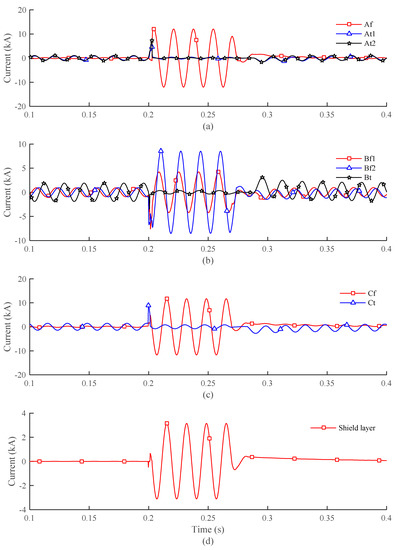
Figure 10.
Current distribution in each phase of the HTS cable: (a) current in phase A that consists of one former layer (Af) and two HTS tape layers (At1 and At2); (b) current in phase B that consists of two former layers (Bf1 and Bf2) and one HTS tape layer (Bt); (c) current in phase C that consists of one former layer (Cf) and one HTS tape layer (Ct); and (d) current in the shield layer.
The temperature of each former layer is shown in Figure 11a. Initially, the temperature of each former layer was assumed to be 70 K. The fault occurred at 0.2 s, which caused the rapid increase of current in each phase, resulting in an increase of the former temperature. It was observed that the temperature of the former phase A (Af) was the smallest whereas that of the former phase C (Cf) was highest. The resistances of former layers are shown in Figure 11b–d. Initially, the former resistance of each layer was different because there were differences in the cross-sections. When the fault occurred, the former resistances slightly increased until the fault was cleared. Reduction of the temperature led to a decrease in former resistance. It was shown that the resistance of the former Af was smallest, whereas that of the former Bf1 was highest. The resistance and temperature rise of the former in phase A were the smallest because the cross-section of former phase A was relatively large compared to other former layers. The resistances of formers in phase B and C were similar because they had similar geometries. However, the fault current in phase C was much larger than phase B, which resulted in a higher temperature of former phase C compared to former phase B.
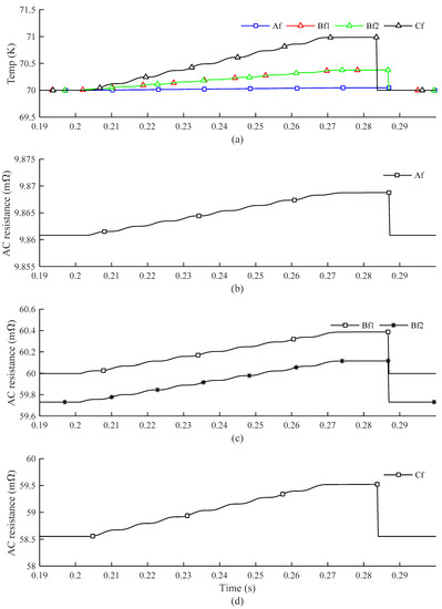
Figure 11.
The temperature of the Cu-former layers and the equivalent AC resistances of each phase in the HTS cable: (a) temperature of the Cu-former layers; (b) resistance of the former Af; (c) resistances of the former Bf1 and Bf2; and (d) resistance of the former Cf.
The AC resistance of the HTS tape layers are shown in Figure 12a. According to [13], the resistance of the HTS tape for the current value over its critical current was measured at about 2.5 mΩ/m and was used in this study. In the normal state, resistance of the HTS tape layer was almost equal to zero. However, that increased significantly when the fault occurred, up to 7.5 Ω for the 3 km length of the HTS cable in this study. The equivalent resistance of a parallel connection of former and HTS tape layers in each phase is shown in Figure 12b. In the normal state, the resistances of the HTS tape layers were much smaller than those of the former layers; however, in the transient state, the HTS tape-layer resistances were much larger than former resistances, which caused the sudden change of equivalent resistance at transient state.
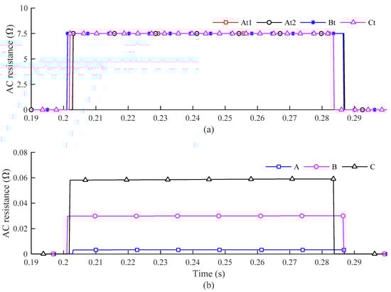
Figure 12.
AC resistances of the HTS tape layers and the equivalent resistance of each phase: (a) resistance of the HTS tape layers; and (b) equivalent resistance of each phase.
4. Conclusions
To protect the HTS tape layers from burning out during the fault, the Cu-former layer was connected in parallel to bypass the transient current, which led to the reduction of heat generation and temperature rise. The use of a Cu-former layer in each phase increased the complexity of HTS cable modeling, especially in the case of modelling the multilayer HTS power cable. This paper proposed a simplified model of the coaxial multilayer HTS power cable with the Cu-former layer in each phase. The idea behind the simplified HTS cable model was to model the change of former layer resistance while the resistances of the HTS tape layers were fixed to maximal values. It was reasonable for these assumptions because the resistances of the HTS tape layers increased significantly during transient conditions due to the quenching phenomenon, which resulted in the flow of transient current into the Cu-former layer. A comparison between experiment simulations of the temperature variations of the former layer validated the proposed HTS cable model. A simplified model of the HTS power cable can be used in transient studies, such as the studies on designing protection of the power system with the integration of the HTS cable. In addition, various optimization methods, such as genetic algorithms, particle swarm optimization, robust optimization, etc., could use the proposed HTS cable model for designing HTS cables in order to find optimal cable parameters to achieve uniform current distribution among multilayer HTS conductors.
Author Contributions
Conceptualization and investigation, T.-T.N. and S.-J.L.; visualization, W.-G.L.; writing—original draft preparation and editing, T.-T.N.; writing—review and supervision, H.-M.K.; project administration, M.P.; funding acquisition, D.W., J.Y. and H.S.Y.
Funding
This work was funded by Korea Electric Power Corporation.
Acknowledgments
The authors would like to thank Seong-Yeol Kang who provided insight and expertise that greatly assisted the research.
Conflicts of Interest
The authors declare no conflict of interest.
References
- Kottonau, D.; de Sousa, W.T.B.; Bock, J.; Noe, M. Design comparisons of concentric three-phase HTS cables. IEEE Trans. Appl. Supercond. 2019, 29, 1. [Google Scholar] [CrossRef]
- Gholizad, B.; Ross, R.; Koopmans, G.; Mousavi Gargari, S.; Smit, J.J.; Ghaffarian Niasar, M.; Meijer, C.; Bucurenciu, A.M. Reliability considerations of electrical insulation systems in superconducting cables. Proc. IEEE Int. Conf. Prop. Appl. Dielectr. Mater. 2018, 2018, 194–197. [Google Scholar]
- McGuckin, P.; Burt, G. Overview and assessment of superconducting technologies for power grid applications. In Proceedings of the 53rd International Universities Power Engineering Conference UPEC, Glasgow, UK, 4–7 September 2018. [Google Scholar]
- Lee, S.J.; Park, M.; Yu, I.K.; Won, Y.; Kwak, Y.; Lee, C. Recent status and progress on HTS cables for AC and DC power transmission in Korea. IEEE Trans. Appl. Supercond. 2018, 28, 1–5. [Google Scholar] [CrossRef]
- Youroukos, E. Economic Feasibility Study of ULMCS. Bachelor’s Thesis, National Technology University of Athens, Athens, Greece, 2007. [Google Scholar]
- Lee, C.; Kim, D.; Kim, S.; Won, D.Y.; Yang, H.S. Thermo-hydraulic analysis on long three-phase coaxial HTS power cable of several kilometers. IEEE Trans. Appl. Supercond. 2019, 8223, 1. [Google Scholar] [CrossRef]
- Samoilenkov, S.V.; Ivanov, S.S.; Lipa, D.; Balashov, N.N.; Altov, V.A.; Zheltov, V.V.; Sytnikov, V.E.; Degtyarenko, P.N.; Kopylov, S.I. Design versions of HTS three-phase cables with the minimized value of AC losses. J. Phys. Conf. Ser. 2018, 969, 012049. [Google Scholar]
- Yagi, M.; Fukushima, H.; Serizawa, M.; Mimura, T.; Nakano, T.; Mukoyama, S.; Takagi, T. Protection against ground faults for a 275-kV HTS cable: An experiment. IEEE Trans. Appl. Supercond. 2018, 28, 1–4. [Google Scholar]
- Bykovsky, N.; Uglietti, D.; Wesche, R.; Bruzzone, P. Damage investigations in the HTS cable prototype after the cycling test in EDIPO. IEEE Trans. Appl. Supercond. 2018, 28. [Google Scholar] [CrossRef]
- Fu, Y.; Tsukamoto, O.; Furuse, M. Copper stabilization of YBCO coated conductor for quench protection. IEEE Trans. Appl. Supercond. 2003, 13, 1780–1783. [Google Scholar] [CrossRef]
- Ishiyama, A.; Wang, X.; Ueda, H.; Yagi, M.; Mukoyama, S.; Kashima, N.; Nagaya, S.; Shiohara, Y. Over-current characteristics of superconducting model cable using YBCO coated conductors. Phys. C Supercond. Appl. 2008, 468, 2041–2045. [Google Scholar] [CrossRef]
- Yagi, M.; Mukoyama, S.; Hirano, H.; Amemiya, N.; Ishiyama, A.; Nagaya, S.; Kashima, N.; Shiohara, Y. Recent development of an HTS power cable using YBCO tapes. Phys. C Supercond. Appl. 2007, 463–465, 1154–1158. [Google Scholar] [CrossRef]
- Kim, S.H.; Seong, K.C.; Lee, C.Y.; Cho, J.W.; Jang, H.M.; Sim, K.D.; Kim, H.J.; Kim, J.H.; Bae, J.H. Design of HTS transmission cable with Cu stabilizer. IEEE Trans. Appl. Supercond. 2006, 16, 1622–1625. [Google Scholar]
- Grilli, F. Numerical modeling of HTS applications. IEEE Trans. Appl. Supercond. 2016, 26, 1–8. [Google Scholar] [CrossRef]
- Doukas, D.I.; Chrysochos, A.I.; Papadopoulos, T.A.; Labridis, D.P.; Harnefors, L.; Velotto, G. Coupled electro-thermal transient analysis of superconducting DC transmission systems using FDTD and VEM modeling. IEEE Trans. Appl. Supercond. 2017, 27, 1–8. [Google Scholar] [CrossRef]
- Fukui, S.; Ogawa, J.; Suzuki, N.; Oka, T.; Sato, T.; Tsukamoto, O.; Takao, T. Numerical analysis of AC loss characteristics of multi-layer HTS cable assembled by coated conductors. IEEE Trans. Appl. Supercond. 2009, 19, 1714–1717. [Google Scholar] [CrossRef]
- Fetisov, S.S.; Zubko, V.V.; Zanegin, S.Y.; Nosov, A.A.; Vysotsky, V.S. Numerical simulation and cold test of a compact 2G HTS power cable. IEEE Trans. Appl. Supercond. 2018, 28. [Google Scholar] [CrossRef]
- Zhou, Z.; Zhu, J.; Li, H.; Qiu, M.; Li, Z.; Ding, K.; Wang, Y. Magnetic-thermal coupling analysis of the cold dielectric high temperature superconducting cable. IEEE Trans. Appl. Supercond. 2013, 23, 3–6. [Google Scholar]
- Conductor, Y.C.; Breschi, M.; Casali, M.; Cavallucci, L.; Marzi, G.D.; Tomassetti, G. Electrothermal analysis of a twisted stacked. IEEE Trans. Appl. Supercond. 2015, 25, 2–6. [Google Scholar]
- Su, R.; Shi, J.; Yan, S.; Li, P.; Wang, W.; Hu, Z.; Zhang, B.; Tang, Y.; Ren, L. Numerical model of HTS cable and its electric-thermal properties. IEEE Trans. Appl. Supercond. 2019, 29. [Google Scholar] [CrossRef]
- Yagi, M.; Masuda, T.; Hayakawa, N.; Hasegawa, T.; Mukoyama, S.; Maruyama, O.; Ohkuma, T.; Ashibe, Y.; Amemiya, N.; Ishiyama, A.; et al. Development of 66 kV and 275 kV Class REBCO HTS power cables. IEEE Trans. Appl. Supercond. 2012, 23, 5401405. [Google Scholar]
- Lee, S.R.; Lee, J.J.; Yoon, J.; Kang, Y.W.; Hur, J. Impact of 154-kV HTS cable to protection systems of the power grid in South Korea. IEEE Trans. Appl. Supercond. 2016, 26, 4–7. [Google Scholar] [CrossRef]
- Lee, S.; Yoon, J.; Lee, B.; Yang, B. Modeling of a 22.9 kV 50 MVA superconducting power cable based on PSCAD/EMTDC for application to the Icheon substation in Korea. Phys. C Supercond. Appl. 2011, 471, 1283–1289. [Google Scholar] [CrossRef]
- Bang, J.H.; Je, H.H.; Kim, J.H.; Sim, K.D.; Cho, J.; Yoon, J.Y.; Park, M.; Yu, I.K. Critical current, critical temperature and magnetic field based EMTDC model component for HTS power cable. IEEE Trans. Appl. Supercond. 2007, 17, 1726–1729. [Google Scholar] [CrossRef]
- Seokho, K.; A-Rong, K.; Ki-Deok, S.; Young-Jin, W.; Daewon, K.; Jun Kyoung, L.; In-Keun, Y.; Jin Geun, K.; Minwon, P.; Jeonwook, C. Development of a PSCAD/EMTDC model component for AC loss characteristic analysis of HTS power cable. IEEE Trans. Appl. Supercond. 2010, 20, 1284–1287. [Google Scholar]
- Seockho, K.; A-Rong, K.; Jeonwook, C.; Minwon, P.; Ki-Deok, S.; Jae-Ho, K.; Jeadeuk, L.; Jin Geun, K.; In-Keun, Y.; Jun Kyoung, L. HTS power cable model component development for PSCAD/EMTDC considering conducting and shield layers. IEEE Trans. Appl. Supercond. 2009, 19, 1785–1788. [Google Scholar]
- Ha, S.K.; Kim, S.K.; Kim, J.G.; Park, M.; Yu, I.K.; Lee, S.; Kim, J.H.; Sim, K. RTDS-based model component development of a tri-axial HTS power cable and transient characteristic analysis. J. Electr. Eng. Technol. 2015, 10, 2083–2088. [Google Scholar] [CrossRef]
- In-Keun, Y.; Minwon, P.; A-Rong, K.; Kideok, S.; Sung-Kyu, K.; Jin-Geun, K.; Sun-Kyoung, H.; Sangjin, L. Transient characteristic analysis of a tri-axial HTS power cable using PSCAD/EMTDC. IEEE Trans. Appl. Supercond. 2012, 23, 5400104. [Google Scholar]
- Magalhaes, A.P.C.; De Barros, M.T.C.; Lima, A.C.S. Earth return admittance effect on underground cable system modeling. IEEE Trans. Power Deliv. 2018, 33, 662–670. [Google Scholar] [CrossRef]
- Wikipedia Contributors Skin Effect. Available online: https://en.wikipedia.org/w/index.php?title=Skin_effect&oldid=865187719 (accessed on 11 February 2019).
- White, G.K.; Collocott, S.J. Heat capacity of reference materials: Cu and W. J. Phys. Chem. Ref. Data 1984, 13, 1251–1257. [Google Scholar] [CrossRef]
- Sim, K. Study on the Design and Transport Characteristics of 22.9 KV, 50 MVA HTS Power Cable. Doctoral Dissertation, Yonsei University, Seoul, Korea, 2011. [Google Scholar]
© 2019 by the authors. Licensee MDPI, Basel, Switzerland. This article is an open access article distributed under the terms and conditions of the Creative Commons Attribution (CC BY) license (http://creativecommons.org/licenses/by/4.0/).