Group Method of Data Handling (GMDH) Lithology Identification Based on Wavelet Analysis and Dimensionality Reduction as Well Log Data Pre-Processing Techniques

Abstract

Although the group method of data handling (GMDH) is a self-organizing metaheuristic neural network capable of developing a classification function using influential input variables, the results can be improved by using some pre-processing steps. In this paper, we propose a joint principal component analysis (PCA) and GMDH (PCA-GMDH) classifier method. We investigated well log data pre-processing techniques composed of dimensionality reduction (DR) and wavelet analysis (WA), using the southern basin of the South Yellow Sea as a case study, with the aim of improving the lithology classification accuracy of the GMDH. Our results showed that the dimensionality reduction method, which is composed of PCA and linear discriminant analysis (LDA), minimized the complexity of the classifier by reducing the number of well log suites to the relevant components and factors. On the other hand, the WA decomposed the well log signals into time-frequency wavelets for the GMDH algorithm. Of all the pre-processing methods, only the PCA was able to significantly increase the classification accuracy rate of the GMDH. Finally, the proposed joint PCA-GMDH classifier not only increased the accuracy but also was able to distinguish between all the classes of lithofacies present in the southern basin of the South Yellow Sea.

1. Introduction

Lithology identification is a fundamental process in reservoir characterization and formation evaluation. Usually, lithofacies are determined by either direct visualization of core samples or manual interpretation of well logs, by correlating similar physical characteristics of reservoir formations. These conventional methods for determining the lithology of the heterogeneous reservoir are time-consuming, labor intensive, and unreliable, since it is as a consequence of the intuition of geologists and log analysts [1,2,3,4].

To overcome these challenges, researchers have tried to introduce cross-plotting as a statistical method on well logs [5,6,7,8]. However, cross-plotting was found to be unable to fully expose the relationship that may exist within well log data [9]. Interpretation from the cross-plot is similarly reliant on the experience of log analysts [10,11]. With the current computational power and the increasing number of well log tools, it has become necessary to automate the process of lithology determination, by minimizing the impact of human interference that can lead to biased and multiple interpretations [12,13,14].

To achieve this, the application of machine-learning algorithms has proven to be a reliable and adaptive approach in identifying lithofacies in the subsurface [15]. To date, the notably common algorithms employed in classifying lithology include the artificial neural network (ANN) and the support vector machine (SVM). The capability of the ANN and the SVM have been evidently portrayed by Al-Anazi and Gates [16,17], Deng et al. [18], Sebtosheikh et al. [19], and, Xie et al. [15]. In addition, an attempt was made by 20. Konaté et al. [20] to improve the accuracy of the ANN and the SVM classifiers using the dimensionality reduction techniques of principal component analysis (PCA) and linear discriminant analysis (LDA). Tian et al. [21] presented a lithology recognition approach using extreme learning machine (ELM).

It is important to mention that, in order to achieve the desired outcome for the ANN, SVM, and ELM machine-learning algorithms, both constant model parameter adjustments and a form of human interference are required. Therefore, there is a high possibility of the model to converge at local minima. Authors, such as Saporetti et al. [22], have avoided this limitation by combining differential evolution search algorithms with ELM to select the optimal learning parameters of ELM lithology classification.

The group method of data handling (GMDH) algorithm has been identified in the literature to be a promising alternative to address this shortcoming. The reason is that the GMDH algorithm does not rely on a constant adjustment of training parameters, before generating an optimal result. That is, there is little manual tasking in the GMDH modelling process. This is because the iterative tuning of the network parameters, optimum model structure, and number of layers and neurons in the hidden layers, are determined automatically due to its self-organizing nature. In effect, the GMDH model generates a polynomial functional structure using a selection of influential input variables [23,24]. Therefore, it must be acknowledged that the outcome from the GMDH model is significantly dependent on the nature of the inputs.

Generally, input variables of well logs can exhibit relationships between each other. This leads to the presence of multiple collinearities, which must be removed from the model development to improve the accuracy of the model. In this regard, dimensionality reduction methods are capable of reducing the set of well logs and the complexity of the model by transforming well logs into relevant or principal components, and discriminant factors. Here, all redundant well logs are removed when the dimensionality reduction technique is employed. Furthermore, the time-frequency information can be extracted from well log signals, using wavelet analysis by decomposing the signals into a series of wavelets having a different scale and position to improve the learning capacity of the model.

In this paper, we initially developed a GMDH model that can detect the various lithofacies of the southern basin of the South Yellow Sea, using well logs. In addition, the well log data pre-processing techniques of wavelet analysis, principal component analysis (PCA), and linear discriminant analysis (LDA), as dimensionality reduction methods, were presented with the aim of improving the accuracy of GMDH classification.

2. Data Description

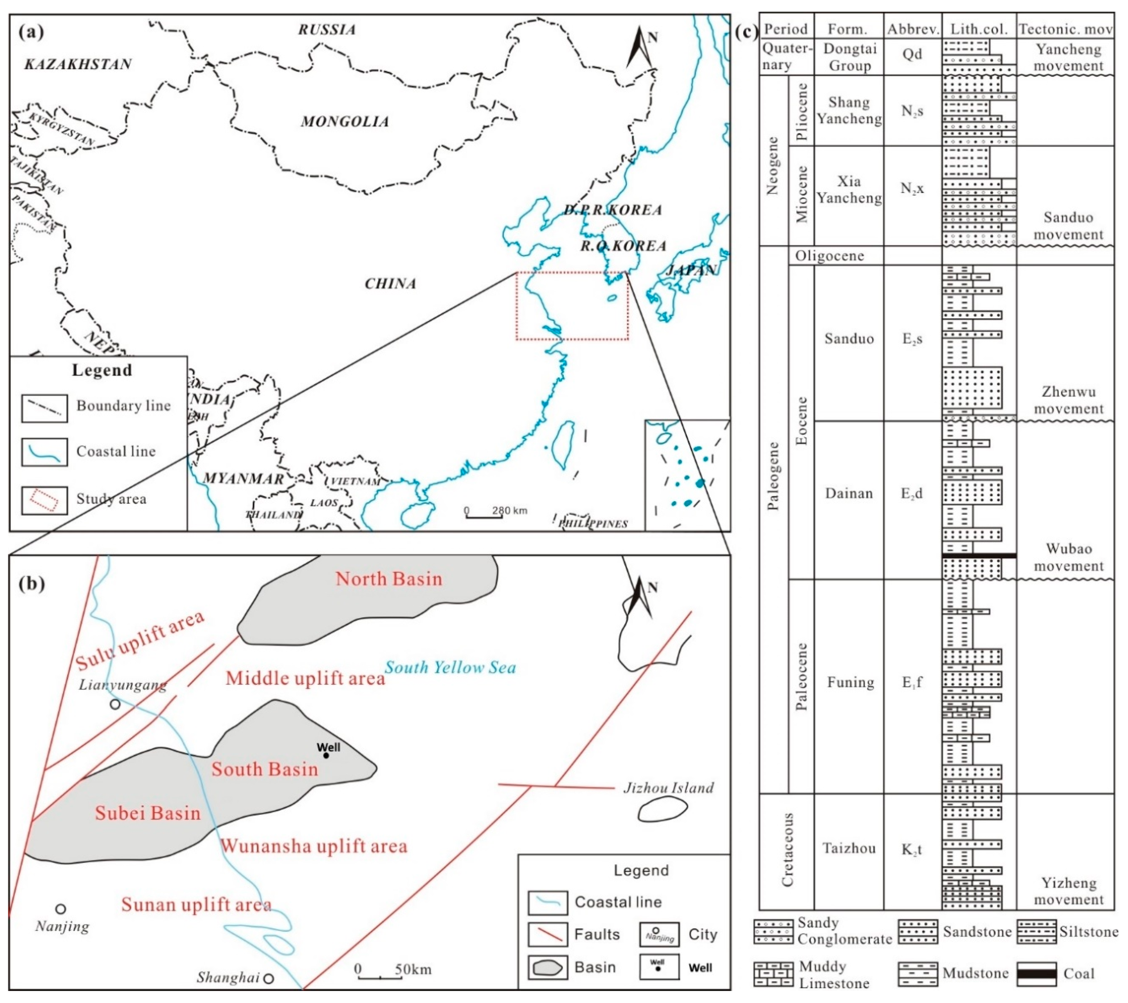
The South Yellow Sea basin is a south-west oriented rift depression basin, located between the Subei basin and Korea peninsular [25,26,27], as shown in Figure 1a. The Southern basin was created from a central uplift, dividing the South Yellow Sea basin into two (Figure 1b). A 1350–2750 m exploratory well having a suite of five well logs and 10,127 core lithology data elements of the southern basin of the South Yellow Sea were considered for this research (Figure 1b). The lithology of the southern basin is composed of sandy conglomerate, siltstone, muddy limestone, mudstone, and coal [28,29], as represented in Figure 1c.

Table 1. Details of the lithology data used in this study.

Lithology	Total Sample Data	Class Assigned
Sandy conglomerate	98	1
Sandstone	548	2
Siltstone	1118	3
Mudstone	8276	4
Muddy limestone	52	5
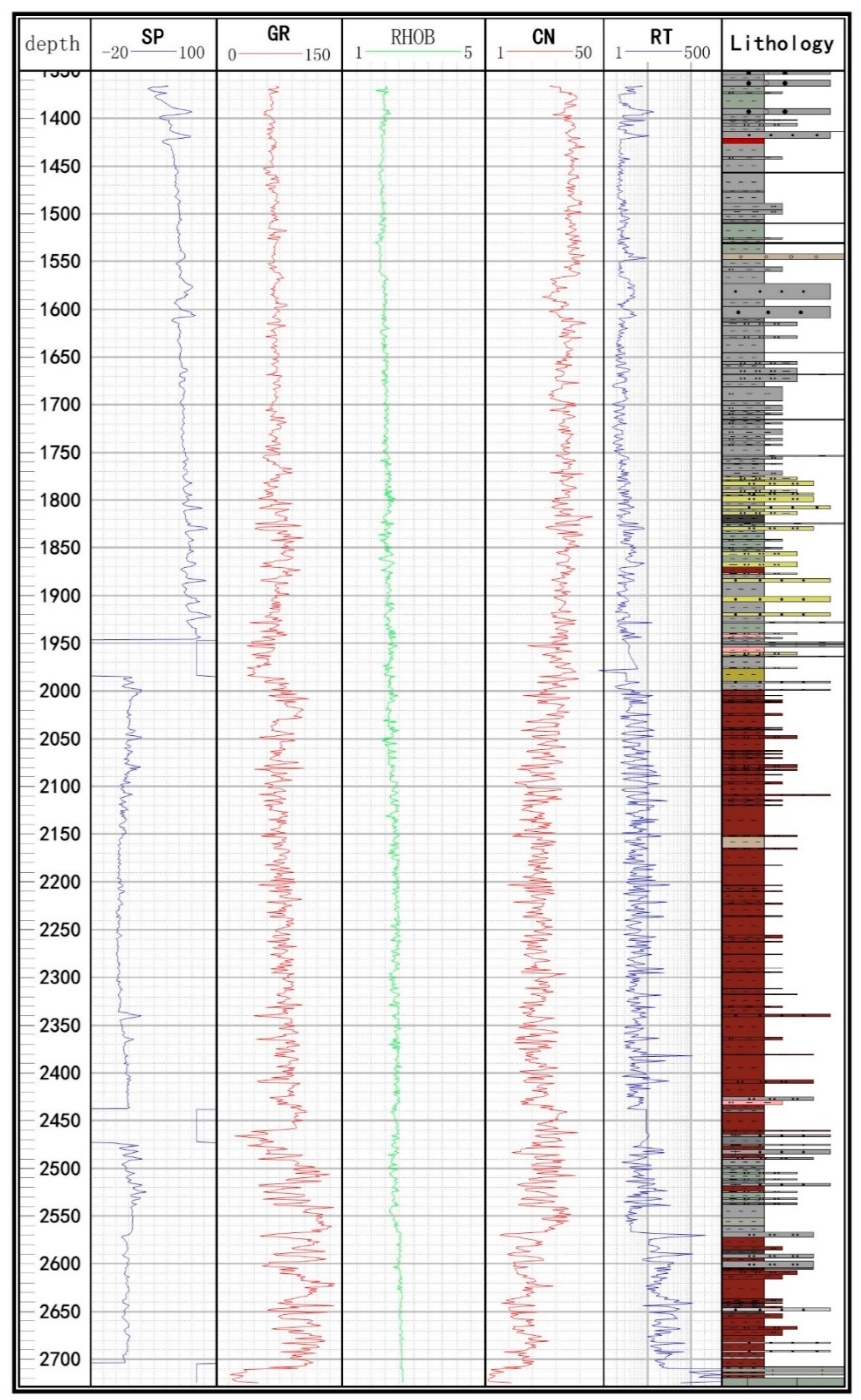
Coal	35	6

summarizes the details of the core lithofacies identified, and considered as the output variable. The log suite that served as the input variables—consisting of bulk density (RHOB), gamma ray (GR), spontaneous potential (SP), compensated neutron (CN), and resistivity (RT)—were used in the development of the GMDH classifiers (Figure 2). In this study, the well log data were sampled at an approximate interval of 0.14 m.

3. Methods

3.1. Group Method of Data Handling (GMDH)

GMDH is based on the search algorithm that sorts out the optimal representation of a polynomial support function, which describes the functional form of the given data according to a specified criterion [23,24]. The structure of GMDH comprises of an input layer, which receives the input variables, multiple hidden layers, and an output layer, which in this case represents the lithology.

Given a set of data with input and output variables of $x_i=\left(x_{i1},x_{i2},\dots ,x_{iN}\right)$ and $y_i=\left(y_{i1},y_{i2},\dots ,y_{iM}\right)$, GMDH can create a relationship between the output and inputs represented as Equation (1).

$$y_i=f\left(x_{i1},x_{i2},\dots ,x_{iN}\right)$$

(1)

The GMDH algorithm is trained to classify the observed values for each input variable.

$$C_i=f_C\left(x_{i1},x_{i2},\dots ,x_{iN}\right)$$

(2)

The difference in the square between $y_i$ and $C_i$ is minimized [30] as:

$$E={{\displaystyle \sum _{i=1}^N\left[f_C\left(x_{i1},x_{i2},\dots ,x_{iN}\right)-y_i\right]}}^2.$$

(3)

An input-output variable equation based on the Volterra–Kolmogorov–Gabor (VKG) polynomial can be built by GMDH [24].

$$C_i=a_o+{\displaystyle \sum _{i=1}^N{a}_i{x}_i+}{\displaystyle \sum _{i=1}^N{\displaystyle \sum _{j=1}^N{a}_{ij}{x}_i{x}_j}+}{\displaystyle \sum _{i=1}^N{\displaystyle \sum _{j=1}^N{\displaystyle \sum _{k=1}^N{a}_{ijk}{x}_i{x}_j{x}_k+\dots }}}$$

(4)

Equation (4) can be simplified using the partial quadratic polynomial system as [31]:

$$C_i=G\left(x_i,x_j\right)=a_o+a_1{x}_i+a_2{x}_i+a_3{x}_i+a_4{x}_i+a_5{x}_i{x}_j$$

(5)

where $C_i$ is the classified lithology, $a$ is the coefficient of the polynomial set by the algorithm, and x is the well log parameter function. From Equation (3), the objective of GMDH is to minimize the value of E by solving for the parameters from multiple regression, using the least squares method to determine the following matrix A [32].

$$A=Y^{{\rm T}}Y$$

(6)

whereby,

$$Y=\left(\begin{array}{ccc}1& x_i& \begin{array}{cc}{x}_j& \begin{array}{cc}{x}_i{x}_j& x_i^2{x}_j^2\end{array}\end{array}\end{array}\right)$$

(7)

then matrix A becomes

$$A=\left(\begin{array}{cccc}\begin{array}{l}1\\ x_i\\ x_j\\ x_i{x}_j\\ x_i^2\\ x_j^2\end{array}& \begin{array}{l}{x}_i\\ x_i^2\\ x_i{x}_j\\ x_i^2{x}_j\\ x_i^3\\ x_i{x}_j^2\end{array}& \begin{array}{l}{x}_j\\ x_i{x}_j\\ x_j^2\\ x_i{x}_j^2\\ x_i^2{x}_j\\ x_j^3\end{array}& \begin{array}{cc}\begin{array}{l}{x}_i{x}_j\\ x_i^2{x}_j\\ x_i^2{x}_j\\ x_i^2{x}_j^2\\ x_i^3{x}_j\\ x_i{x}_j^3\end{array}& \begin{array}{cc}\begin{array}{l}{x}_i^2\\ x_i^3\\ x_i^2{x}_j\\ x_i^3{x}_j\\ x_j^4\\ x_i^2{x}_j^2\end{array}& \begin{array}{l}{x}_j^2\\ x_i{x}_j^2\\ x_j^3\\ x_i{x}_j^3\\ x_i^2{x}_j^2\\ x_j^4\end{array}\end{array}\end{array}\end{array}\right)$$

(8)

assuming

$$X=\left(\begin{array}{ccc}{a}_o& a_1& \begin{array}{cc}{a}_2& \begin{array}{cc}{a}_3{a}_4& a_5\end{array}\end{array}\end{array}\right)$$

(9)

and

$$b={\left(yY\right)}^T$$

(10)

then,

$${\displaystyle \sum _{i=1}^{N}AX={\displaystyle \sum _{i=1}^{N}b}}.$$

(11)

3.2. Principal Component Analysis

Principal component analysis (PCA) is a statistical technique introduced by Pearson [33] as a tool for simplifying the complexity of high-dimensional data, while maintaining its variance. This is achieved through an orthogonal projection or transformation of the data, which is having correlated variables into uncorrelated variables known as principal components (PC). When performing PCA, a covariance matrix of the well log data was initially constructed and the eigenvectors of the matrix were then computed. The eigenvectors having the largest eigenvalues were used in place of the original well log data, as they represent the greater portion of the variance of the original well log data. The first PC minimizes the distance between the data set and its transformation while maximizing the variance of the transformed data points. The succeeding PCs are similarly computed and they have to be uncorrelated with the previous PC. In this paper, PCA was performed in IBM SPSS Statistics software v24.0.

3.3. Linear Discriminant Analysis

The linear discriminant analysis (LDA) method performs dimensionality reduction by finding a linear combination of features, which characterizes or separates two or more classes of object, while preserving as much of the class discriminatory information as possible. LDA explicitly attempts to model the difference between the classes of data, while PCA does not consider the differences, but considers the similarities in class instead. LDA was also conducted in IBM SPSS Statistics software v24.0.

3.4. Discrete Wavelet Transform

The wavelet transform is the process applied on signals to obtain details in the form of frequency and time. The time-frequency transform of a signal f(t) is represented as [34]:

$$f\left(t\right)\leftrightarrow \psi \left(a,b\right)={\displaystyle {\int }_{-\infty }^{\infty }\overline{{\psi }_{ab}}}\cdot f\left(t\right)dt$$

(12)

where a is the frequency or the scale factor that determines the wavelength, b is the position or the shift of the signal, ${\psi }_{ab}$ is the analyzing function, $\overline{{\psi }_{ab}}$ is the complex conjugate, and $f\left(t\right)$ is the original well log signal. In this study, discrete wavelet transform (DWT) was used instead of continuous wavelet transform because it requires less computation time, is simpler to develop, and it is more efficient for practical cases.

In the wavelet transform, the analyzing function can be expressed as [34]:

$${\psi }_{ab}\left(t\right)=a^{\frac{-1}{2}}\psi \left(\frac{t-b}{a}\right).$$

(13)

A DWT is a type of wavelet transform where shifts and dilations are not constantly varied [35]. This is expressed in Equation (14) [34].

$$W_x\left(a,b\right)=\frac{1}{\sqrt{a^j}}{\displaystyle {\int }_{-\infty }^{\infty }\overline{\psi }\left(\frac{t-b}{a^j}\right)}\cdot f\left(t\right)dt$$

(14)

In DWT, a and b can be defined as functions of level j and position k and t is time.

$$a=2^j,b=a\cdot k$$

(15)

Analyzing the function $\psi$ becomes

$${\psi }_{j,k}=\frac{1}{\sqrt{2^j}}\psi \left(2^j\cdot t-k\right)$$

(16)

where $\psi$ is the mother wavelet and ${\psi }_{j,k}$ becomes the daughter wavelet [34]. The results from DWT decomposition generate an approximation wavelet coefficient (cA) and detailed wavelet coefficients (cD), with the aim of extracting additional information from the well log signals to improve the learning capacity of the GMDH algorithm [35].

4. Results and Discussion

4.1. Principal Component Analysis

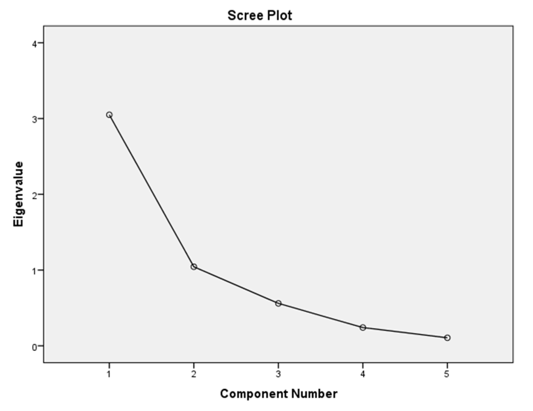
The results from the PCA as shown in

Table 2. Performance of principal component analysis (PCA) on well log data of the southern basin of the South Yellow Sea.

Component	Eigenvalues	% of Variance	Cumulative %
1	3.049343	60.98685	60.98685
2	1.043544	20.87087	81.85773
3	0.560054	11.20109	93.05881
4	0.240918	4.818351	97.87716
5	0.106142	2.122836	100

indicate that component 1 and component 2 can retain and interpret a greater portion of the total variance of the entire well logs considered in this study. This assertion is based on the Kaiser criterion [36], which reveals that components having eigenvalues of more than 1 can preserve and represent the total information of the data being reduced. Therefore, components 1 and 2 were selected since their eigenvalues are more than 1. From Table 2, component 1 and component 2 observed an eigenvalue of 81.858% of the total variance of the well log suite. Component 1 accounted for 60.99%, while component 2 represented 20.87% of the total variance. 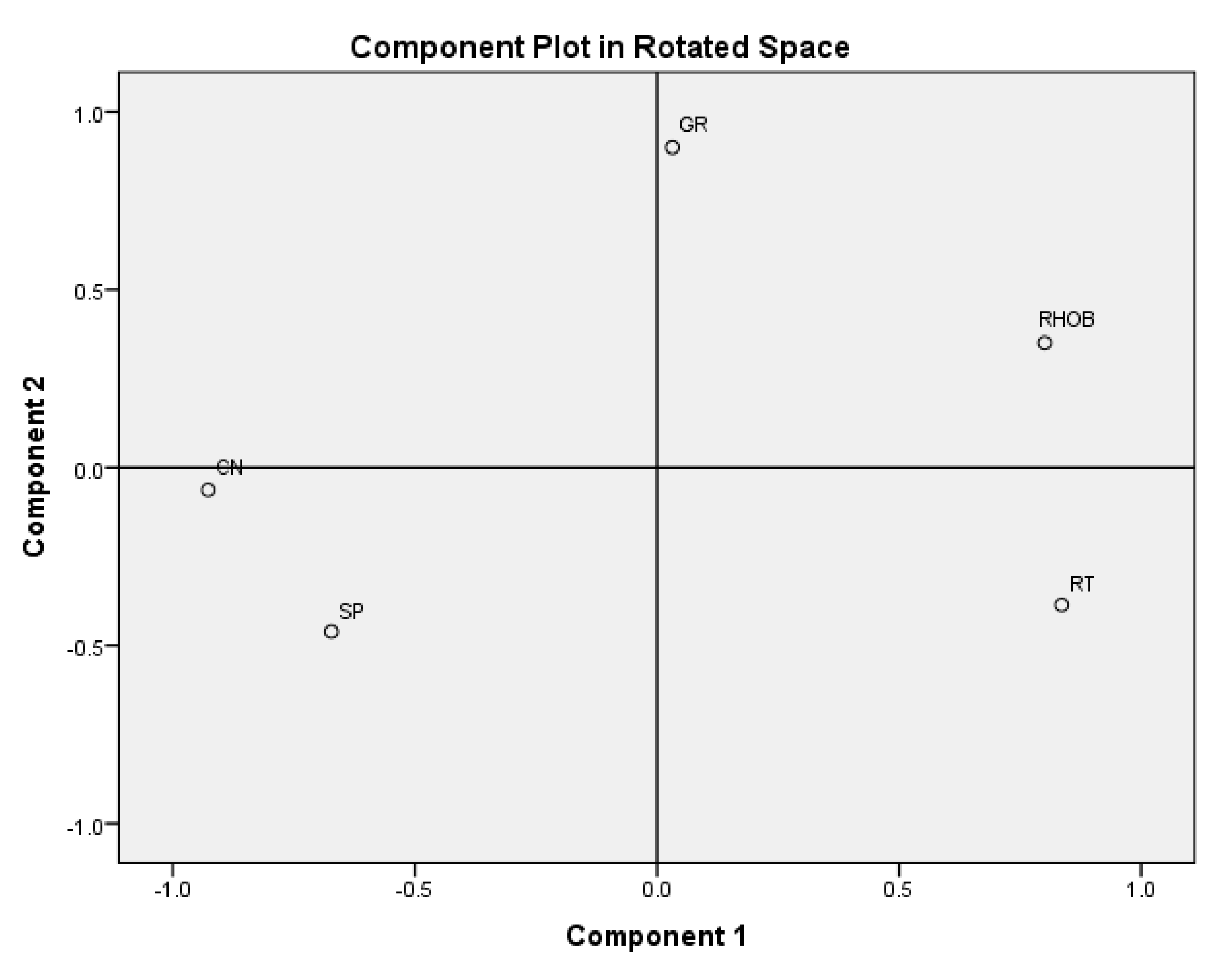An observation made from the scree plot in Figure 3 revealed a change in the direction of the line after component 2. This confirms the fact that only component 1 and component 2 are the meaningful variance from the suite of considered well logs. The selected PCs were further rotated to assess their correlation to each well log parameter in Figure 4. Details of the linear relationship between the well logs and the principal components extracted are listed in

Table 3. Correlation between well logs and selected principal components.

Well Log	Component
	1	2
RHOB	0.935	0.049
CN	−0.911	0.239
SP	−0.868	−0.186
RT	0.6	−0.599
GR	0.482	0.768

. RHOB, CN, and SP had high correlation values with component 1, while GR observed a high correlation value of 0.768 with component 2 (Table 3). Therefore, components 1 and 2 replaced the well log parameters as inputs for the hybrid PCA-GMDH lithology classifier.

4.2. Linear Discriminant Analysis

Table 4. Performance of Linear Discriminant Analysis (LDA) on well log data of the southern basin of the South Yellow Sea.

Discriminant Function	Eigenvalue	% of Variance	Cumulative %
1	4.5939	75.4	75.4
2	2.2632	15.2	90.6
3	1.5648	7.0	97.6
4	0.8895	2.3	99.9
5	0.0217	0.1	100

summarizes the results from LDA on the five well logs and the core lithology data. It was found that three discriminant factors had eigenvalues greater than 1. Specifically, factor 1, 2, and 3 obtained eigenvalues of 4.5939, 2.2632, and 1.5648 respectively (Table 4). The three discriminant factors explained 97.6% variance of the entire well logs considered. Factor 1 accounted for 75.4%, factor 2 explained 15.2%, and factor 3 explained 7% of the total variance of the well logs. The coefficient of the well logs in each discriminant function is listed in

Table 5. The coefficient of discriminant factors.

Well Log	Discriminant Function
	1	2	3
RHOB	0.067	1.931	0.048
GR	0.318	−0.527	−0.386
SP	−1.23	−0.055	−0.153
CN	1.146	1.831	1.078
RT	−0.192	0.62	0.127

. It is important to note that the larger the coefficient in the discriminant function, the more that well log parameter will contribute to discriminating between the various classes. Therefore, it can be seen from Table 5 that the CN well log contributed significantly to all of the three discriminant functions. The joint LDA-GMDH classification model was generated from discriminant function 1, 2, and 3 input variables.

4.3. Discrete Wavelet Transform

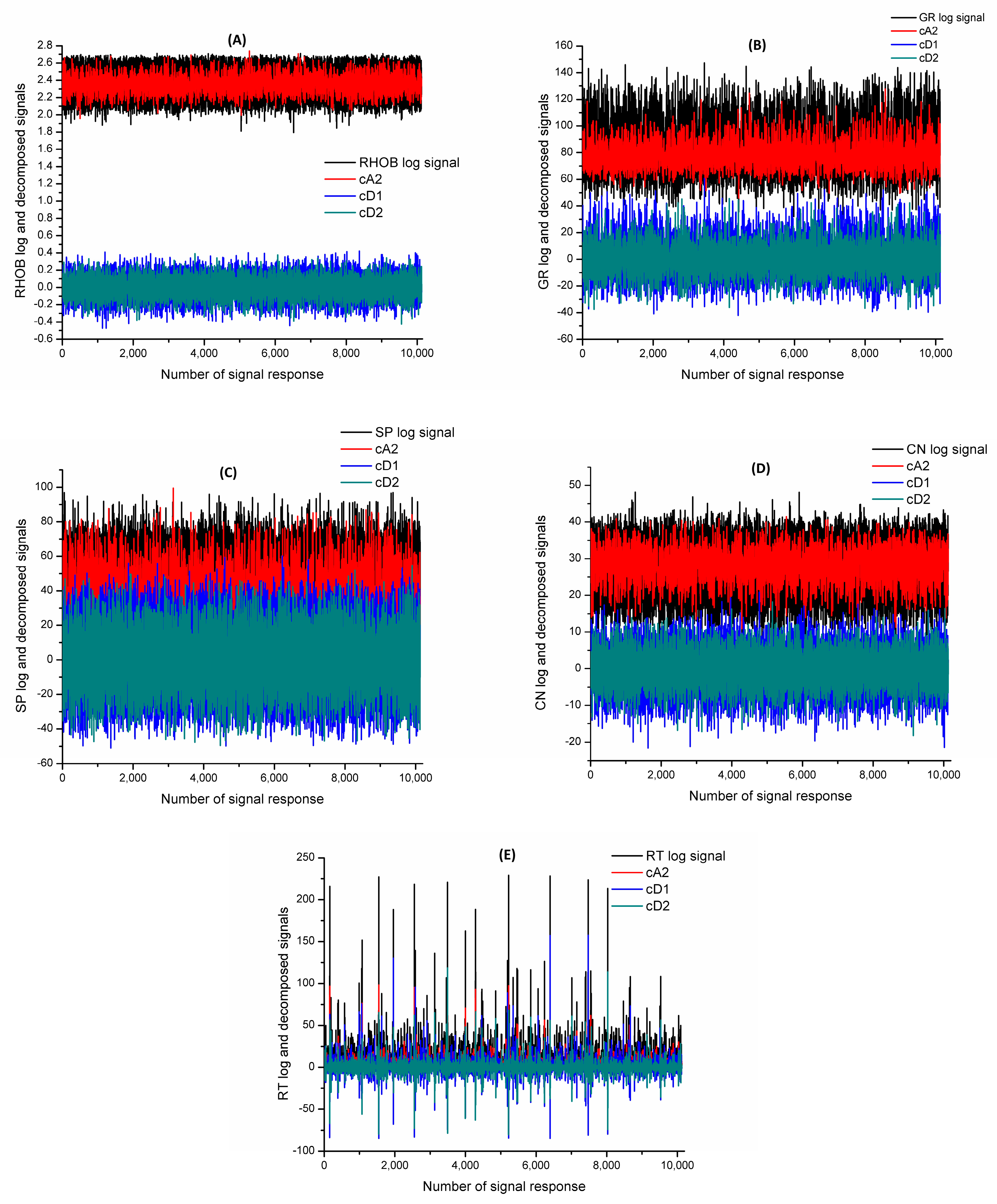
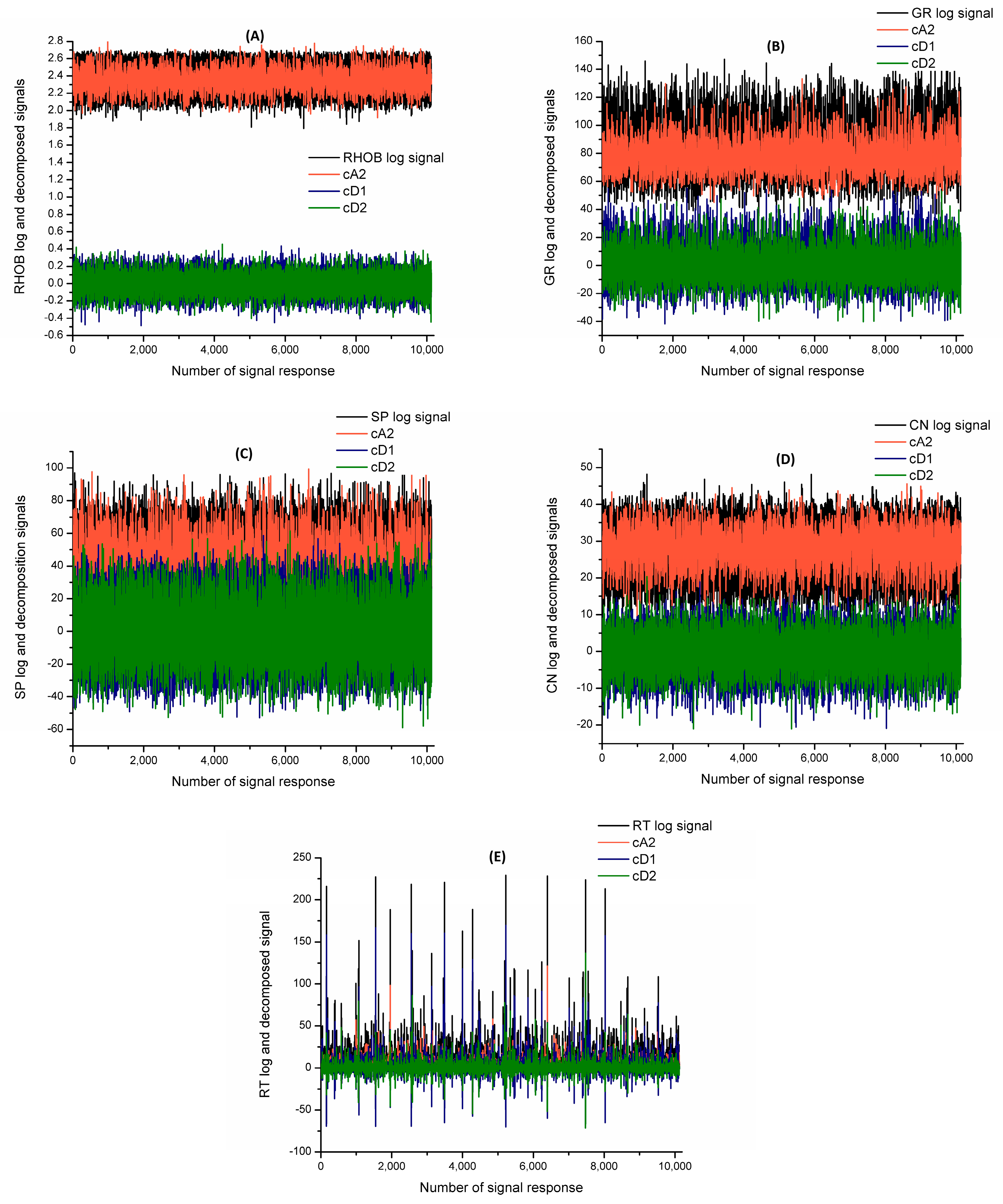
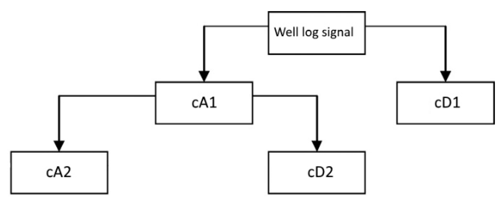
This study performed DWT using wavelet functions of Daubechies (db), ReverseBior (rbio), and Symlets (sym) to decompose the well log signals [34,35] in the wavelet toolbox in Matlab R2016a. A two-level decomposition using the db-2, rbio-2.2, and sym-2 wavelet function generated an approximation wavelet (cA2) and two detailed wavelets (cD1 and cD2). The well log signals were initially decomposed into low- and high-frequency components. The approximation value from the initial decomposition (cA1) is the low-frequency component, while the detail value of the signal (cD1) is the high-frequency component. From Figure 5, the two-level decomposition is a further breakdown of the low-frequency component. The low-frequency component of most signals is the most important; however, the high-frequency component plays the role of an “additive” [37]. Figure 6 and Figure 7 compare the various well log signals and their corresponding approximation (cA2) and detailed (cD1 and cD2) wavelet coefficients. Therefore, each well log was replaced by the generated three wavelet signals as inputs.

4.4. GMDH Classifiers

In this section, GMDH classifiers were developed by selecting 60% of the 10,127 lithology data elements and their corresponding well log signals, principal components, discriminant factors, and wavelet signals as training data. Forty percent (40%) of the data became the benchmark used to assess the trained classifiers, i.e., the testing dataset. The inputs of GMDH were the five well log sets (i.e., RHOB, GR, SP, CN, and RT) trained to identify the various lithofacies. Similarly, component 1 and component 2 were used as inputs to build the PCA-GMDH lithology classifier. For LDA-GMDH, discriminant factors 1, 2, and 3 were the input variables, while 15 wavelet signals comprised of the cA2, cD1, and cD2 for all five well log signals were the input variables for db2-GMDH, rbio2.2-GMDH, and sym2-GMDH. GMDH classification models were coded and implemented in MATLAB R2016a.

The performance of GMDH lithology classification models was assessed based on how accurate they were able to identify the various lithofacies. The optimal GMDH structure was made up of five input neurons, 15 hidden layers with a varying number of hidden neurons in each layer, and lithology as the output (

Table 6. Network structure and equations from GMDH lithology classifier.

Layer	No of Neurons	Equation
1	3	x1 = 2.9 − 3.4(RT) + 3.3(GR) + 0.9(RT × GR) + 3.1(RT)2 − 2.4(GR)2
		x2 = 3.3 + 3.7(CN) − 3.8(CN) + 6.5(SP × CN) − 4.3(CN)2 − 1.2(SP)2
		x3 = 3.9 + 4.7(RT) + 0.6(SP) − 67.4(SP × RT) + 3.2(RT)2 − 0.8(SP)2
2	2	x4 = 13.9 − 5.2(x3) − 1.7(x1) + 1.8(x1·x3) − 0.02(x3)2 − 0.6(x1)2
		x5 = 4 − 5.8(x3) + 4.4(x2) + 1.9(x3·x4) − 0.03(x3)2 − 1.5(x4)2
3	2	x6 = − 4.6 + 2.6(x4) + 5.3(RHOB) − 1.6(RHOB·x4) − 0.09(x4)2 + 0.5(RHOB)2
		x7 = − 3.6 + 2.3(x5) + 4.2(RHOB) − 1.2(RHOB·x5) − 0.09(x5)2 + 0.1(RHOB)2
4	2	x8 = 1.2 + 0.4(x7) − 2.4(SP) + 0.3(SP·x7) + 0.08(x7)2 + 1.7(SP)2
		x9 = − 4.1 + 2.5(x6) + 5(CN) − 1.3(CN·x6) − 0.1(x6)2 − 0.02(CN)2
5	1	x10 = − 0.7 + 0.3(x9) + 0.9(x8) − 1.3(x8·x9) + 0.7(x9)2 + 0.6(x8)2
6	2	x11 = − 0.5 + 0.9(x10) + 1.6(RHOB) − 0.5(RHOB·x10) + 0.05(x10)2 + 0.2(RHOB)2
		x12 = − 1.1 + 1.1(x10) + 5(GR) − 1.5(GR·x10) + 0.07(x10)2 + 1.04(GR)2
7	1	x13 = − 0.6 + 0.08(x12) + 1.2(x11) − 6.2(x11·x12) + 3.2(x12)2 + 3(x11)2
8	2	x14 = 0.9 + 0.62(x13) − 2(SP) + 0.3(SP·x13) + 0.04(x13)2 + 1.2(SP)2
		x15 = − 1.7 + 1.6(x13) + 2.3(CN) − 0.6(CN·x13) − 0.04(x13)2 + 0.07(CN)2
9	1	x16 = − 0.3 − 4.8(x15) + 5.9(x14) − 10.8(x15·x14) + 6.2(x15)2 + 4.6(x14)2
10	1	x17 = − 2.1 + 1.8(x16) + 2.5(CN) − 0.7(CN·x16) − 0.06(x16)2 + 0.09(CN)2
11	1	x18 = − 0.7 + 0.9(x17) + 2.8(RHOB) − 0.7(RHOB·x17) + 0.07(x17)2 − 0.2(RHOB)2
12	1	x19 = 1.4 + 0.4(x18) − 2.3(SP) + 0.4(SP·x18) + 0.06(x18)2 + 0.9(SP)2
13	1	x20 = − 2.3 + 1.8(x19) + 2.9(CN) − 0.7(CN·x19) − 0.07(x19)2 − 0.2(CN)2
14	1	x21 = − 0.04 + 0.96(x20) + 4.4(RT) − 1.1(RT·x20) + 0.01(x20)2 − 1.4(RT)2
15	2	x22 = − 0.5 + 1.1(x21) + 1.7(GR) − 0.5(GR·x21) + 0.01(x21)2 + 0.2(GR)2
		x23 = 0.6 + 0.8(x21) − 0.7(SP) + 0.2(SP·x21) + 0.02(x21)2 − 0.05(SP)2
output	1	Lithology = 0.09 + 13.8(x23) − 12.7(x22) + 94.3(x22·x23) − 49(x23)2 − 45.4(x22)2

). The polynomial equations used to develop the optimal GMDH classification model are summarized in Table 6. It was observed that GMDH using the suite of five well logs achieved a classification accuracy rate of 82.488% and 81.806% for training and testing, respectively.

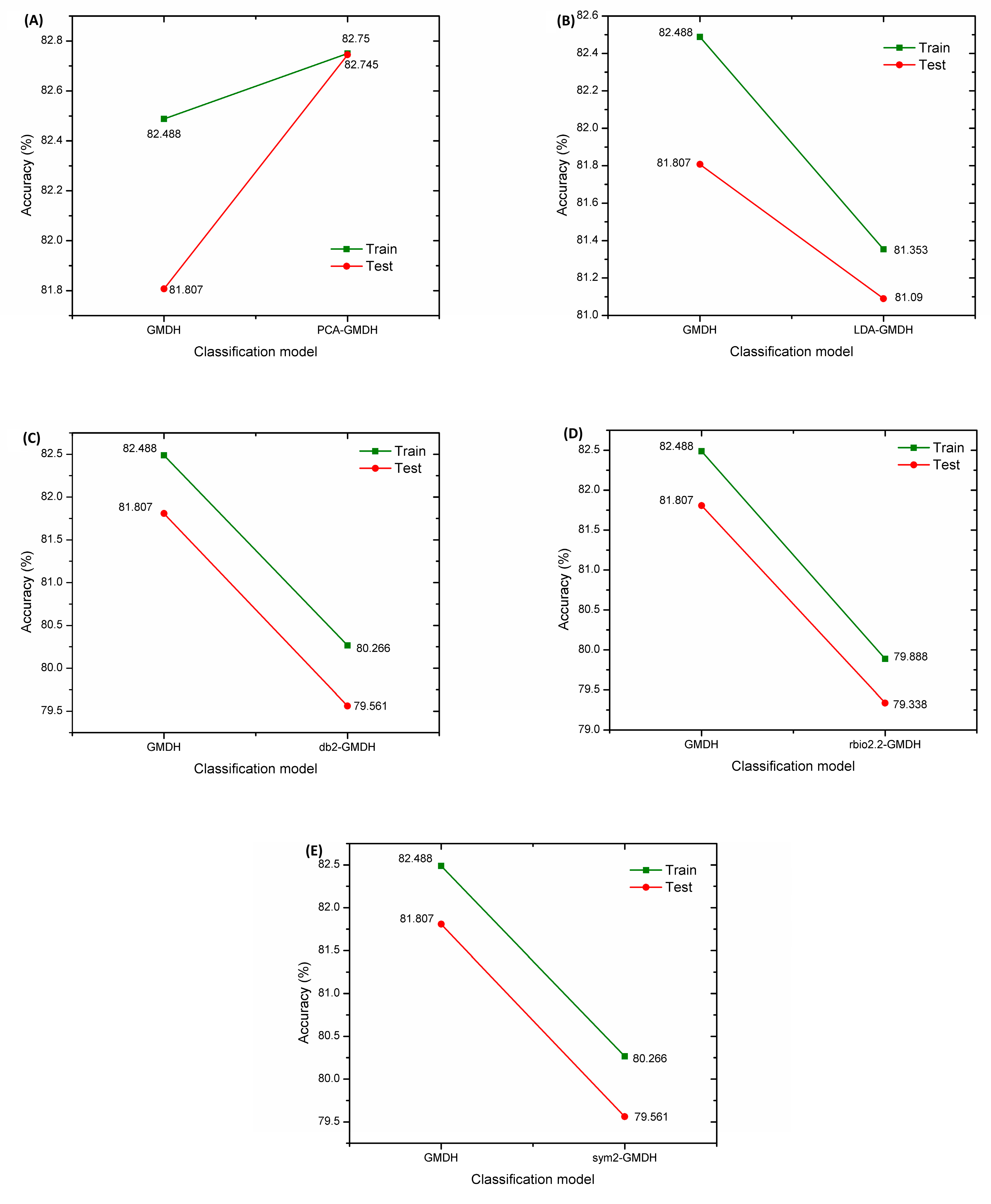
As explained earlier, we conducted a comparative study with PCA-GMDH, LDA-GMDH, db2-GMDH, rbio2.2-GMDH, and sym2-GMDH to see whether the results of the GMDH classification model can be improved. As illustrated in Figure 8A, PCA-GMDH successfully improved the results of GMDH, as it produced classification results having an accuracy rate of 82.75% and 82.745% for training and testing, respectively. When analyzing the outcome from the LDA-GMDH, db2-GMDH, rbio2.2-GMDH, and sym2-GMDH classifiers, it was identified that, for the data used in this study, the LDA and DWT pre-processing techniques accounted for a decrease in the performance of GMDH. This means that LDA-GMDH, db2-GMDH, rbio2.2-GMDH, and sym2-GMDH could not perform better than GMDH. From Figure 8B, LDA-GMDH obtained an accuracy rate of 81.353% and 81.09% for training and testing, respectively. According to Figure 8C–E, db2-GMDH and sym2-GMDH had a similar accuracy output of 80.266% and 79.561%, while rbio2.2-GMDH achieved 79.888% and 79.338% for training and testing, respectively.

A detailed assessment of how each model misclassified the various lithofacies is summarized in

Table 7. Misclassification of the lithofacies.

Classifiers	% Misclassification
	Sandy Conglomerate	Sandstone	Siltstone	Mudstone	Muddy Limestone	Coal
GMDH	74.49	67.88	18.34	3.89	92.31	100.00
PCA-GMDH	66.33	67.52	21.29	3.33	90.38	94.29
LDA-GMDH	98.98	84.67	14.04	5.91	96.15	100.00
db2-GMDH	98.98	84.67	14.04	5.91	96.15	100.00
rbio2.2-GMDH	100.00	91.24	17.53	5.91	100.00	100.00
sym2-GMDH	98.98	84.67	14.04	5.91	96.15	100.00

. According to Table 7, all the GMDH models performed significantly well when identifying siltstone and mudstone facies. This is attributed to the large amount of siltstone and mudstone that were present in the study area. Lithofacies, such as sandy conglomerate, muddy limestone, and coal, were often misclassified by db2-GMDH, sym2-GMDH, and rbio2.2-GMDH. GMDH and LDA-GMDH failed to recognize coal facies. Furthermore, PCA-GMDH was able to distinguish between all the present classes of lithology, as shown in Table 7.

5. Conclusions

The self-organizing ability of the GMDH algorithm, whereby it does not rely on any human interference to adjust its model parameters, was successfully implemented to identify lithofacies present in the southern basin of the South Yellow Sea. This study explored the impact of the pre-processing techniques of PCA and LDA as dimensional-reduction methods, and wavelet analysis, regarding the performance of GMDH lithology classification.

The well log sets of five parameters were reduced to two principal components and three discriminant factors by PCA and LDA, respectively, while maintaining most of the total variance of the well log data. The discrete wavelet transform decomposed each well log signal into approximation (cA2) and detailed wavelet (cD1, cD2) signals.

Evaluating the GMDH lithology classification models revealed that PCA-GMDH achieved an improved accuracy rate, when compared with GMDH. For the purpose of this study, however, LDA-GMDH, db2-GMDH, sym2-GMDH, and rbio2.2-GMDH were unable to improve the results of GMDH.

Among the facies present in the southern basin of the South Yellow Sea, siltstone and mudstone were the accurately identified facies. Siltstone and mudstone were easily detected as a consequence of their large quantities. In the study area, PCA-GMDH presented the ability to differentiate between the various classes.

To conclude, based on the findings of this study, PCA is the well log data pre-processing technique that can improve the performance of GMDH, and can be adopted as the lithology classification model for the rest of the wells in the southern basin of the South Yellow Sea.

References

1. Chang, H.C.; Kopaska-Merkel, D.C.; Chen, H.C.; Durrans, S.R. Lithofacies identification using multiple adaptive resonance theory neural networks and group decision expert system. Comput. Geosci. 2000, 26, 591–601. [Google Scholar] [CrossRef]
2. Maiti, S.; Tiwari, R.K. Neural network modeling and an uncertainty analysis in Bayesian framework: A case study from the KTB borehole site. J. Geophys. Res. Solid Earth 2010, 115. [Google Scholar] [CrossRef] [Green Version]
3. Saggaf, M.M.; Nebrija, L. A fuzzy logic approach for the estimation of facies from wire-line logs. AAPG Bull. 2003, 87, 1223–1240. [Google Scholar] [CrossRef]
4. Ehsan, M.; Gu, H.; Akhtar, M.M.; Abbasi, S.S.; Ullah, Z. Identification of hydrocarbon potential of talhar shale: Member of lower goru formation by using well logs derived parameters, southern lower indus basin, Pakistan. J. Earth Sci. 2018, 29, 587–593. [Google Scholar] [CrossRef]
5. Pechnig, R.; Bartetzko, A.; Delius, H. Effects of compositional and structural variations on log responses in igneous and metamorphic rocks. In Proceedings of the AGU Fall Meeting, San Francisco, CA, USA, 10–14 December 2001. Abstract V32C-0988. [Google Scholar]
6. Pechnig, R.; Delius, H.; Bartetzko, A. Effect of compositional variations on log responses of igneous and metamorphic rocks, Chapter 2: Acid and intermediate rocks. In Petrophysical Properties of Crystalline Rocks; Harvey, P.K., Brewer, T.S., Pezard, P.A., Petrov, V.A., Eds.; Geological Society Special Publications: London, UK, 2005; pp. 279–300. [Google Scholar]
7. Bartetzko, A.; Delius, H.; Pechnig, R. Effect of compositional and structural variations on log responses of igneous and metamorphic rocks, Chapter 1: Mafic rocks. In Petrophysical Properties of Crystalline Rocks; Harvey, P.K., Brewer, T.S., Pezard, P.A., Petrov, V.A., Eds.; Geological Society Special Publications: London, UK, 2005; pp. 255–278. [Google Scholar]
8. Salim, A.M.A.; Pan, H.P.; Luo, M.; Zhou, F. Integrated log interpretation in the Chinese continental scientific drilling main hole (Eastern China): Lithology and mineralization. J. Appl. Sci. 2008, 8, 3593–3602. [Google Scholar] [CrossRef]
9. Kassenaar, J.D.C. An application of principal components analysis to borehole geophysical data. In Proceedings of the Fourth International Symposium on Borehole Geophysics for Minerals, Geotechnical and Groundwater Applications, Toronto, ON, Canada, 18–22 August 1991; pp. 211–218. [Google Scholar]
10. Saggaf, M.M.; Nebrija, E.L. Estimation of lithologies and depositional facies from wire-line logs. AAPG Bull. 2008, 4, 1633–1646. [Google Scholar]
11. Amirgaliev, E.; Isabaev, Z.; Iskakov, S.; Kuchin, Y.; Muhamedyev, R.; Muhamedyeva, E.; Yakunin, K. Recognition of rocks at uranium deposits by using a few methods of machine learning. Soft Comput. Mach. Learn. Adv. Intell. Syst. Comput. 2014, 273, 33–40. [Google Scholar]
12. Horrocks, T.; Holden, E.J.; Wedge, D. Evaluation of automated lithology classification architectures using highly-sampled wireline logs for coal exploration. Comput. Geosci. 2015, 83, 209–218. [Google Scholar] [CrossRef]
13. Yang, H.; Pan, H.; Ma, H.; Konaté, A.A.; Yao, J.; Guo, B. Performance of the synergetic wavelet transform and modified k-means clustering in lithology classification using nuclear log. J. Petrol. Sci. Eng. 2016, 144, 1–9. [Google Scholar] [CrossRef]
14. Borsaru, M.; Zhou, B.; Aizawa, T.; Karashima, H.; Hashimoto, T. Automated lithology prediction from pgnaa and other geophysical logs. Appl. Radiat. Isotopes 2006, 64, 272–282. [Google Scholar] [CrossRef]
15. Xie, Y.; Zhu, C.; Zhou, W.; Li, Z.; Tu, M. Evaluation of machine learning methods for formation lithology identification: A comparison of tuning processes and model performances. J. Petrol. Sci. Eng. 2018, 139, 182–193. [Google Scholar] [CrossRef]
16. Al-Anazi, A.; Gates, I.D. A support vector machine algorithm to classify lithofacies and model permeability in heterogeneous reservoirs. Eng. Geol. 2010, 114, 267–277. [Google Scholar] [CrossRef]
17. Al-Anazi, A.; Gates, I.D. On the capability of support vector machines to classify lithology from well logs. Nat. Resour. Res. 2010, 19, 125–139. [Google Scholar] [CrossRef]
18. Deng, C.; Pan, H.; Fang, S.; Konaté, A.A.; Qin, R. Support vector machine as an alternative method for lithology classification of crystalline rocks. J. Geophys. Eng. 2017, 14, 341–349. [Google Scholar] [CrossRef]
19. Sebtosheikh, M.A.; Motafakkerfard, R.; Riahi, M.A.; Moradi, S. Separating well log data to train support vector machines for lithology prediction in a heterogeneous carbonate reservoir. Iran. J. Oil Gas Sci. Technol. 2015, 4, 1–14. [Google Scholar]
20. Konaté, A.A.; Pan, H.; Ma, H.; Cao, X.; Ziggah, Y.Y.; Oloo, M.; Khan, N. Application of dimensionality reduction technique to improve geo-physical log data classification performance in crystalline rocks. J. Pet. Sci. Eng. 2015, 133, 633–645. [Google Scholar] [CrossRef]
21. Tian, Y.; Pan, H.; Liu, X.; Cheng, G. Lithofacies recognition based on extreme learning machine. Appl. Mech. Mater. 2013, 241, 1762–1767. [Google Scholar] [CrossRef]
22. Saporetti, C.M.; Duarte, G.R.; Fonseca, T.L.; Goliatt da Fonseca, L.; Pereira, E. Extreme learning machine combined with a differential evolution algorithm for lithology identification. Rev. Inform. Orica Apl. RITA 2018, 25, 43–56. [Google Scholar] [CrossRef]
23. Ivakhnenko, A.G. The group method of data handling: A rival of the method of stochastic approximation. Sov. Autom. Control 1968, 13, 43–55. [Google Scholar]
24. Ivakhnenko, A.G. Polynomial theory of complex systems. IEEE Trans. Syst. Man Cybern. 1971, 1, 364–378. [Google Scholar] [CrossRef]
25. Yi, S.; Yi, S.; Batten, D.J.; Yun, H.; Park, S.J. Cretaceous and Cenozoic non-marine deposits of the Northern South Yellow Sea Basin, offshore western Korea: Palynostratigraphy and palaeoenvironments. Palaeogeogr. Palaeoclimatol. Palaeoecol. 2003, 191, 15–44. [Google Scholar] [CrossRef]
26. Wu, S.; Ni, X.; Cai, F. Petroleum geological framework and hydrocarbon potential in the Yellow Sea. Chin. J. Oceanol. Limnol. 2008, 26, 23–34. [Google Scholar] [CrossRef]
27. Pang, Y.; Zhang, X.; Xiao, G.; Wen, Z.; Guo, X.; Hou, F.; Zhu, X. Structural and geological characteristics of the south yellow sea basin in lower yangtze block. Geol. Rev. 2016, 62, 604–616. (In Chinese) [Google Scholar]
28. Asante-Okyere, S.; Shen, C.; Ziggah, Y.Y.; Rulegeya, M.M.; Zhu, X. Investigating the predictive performance of gaussian process regression in evaluating reservoir porosity and permeability. Energies 2018, 11, 3261. [Google Scholar] [CrossRef]
29. Gao, D.; Cheng, R.; Shen, Y.; Wang, L.; Hu, X. Weathered and volcanic provenance-sedimentary system and its influence on reservoir quality in the east of the eastern depression, the north yellow sea basin. J. Earth Sci. 2018, 29, 353–368. [Google Scholar] [CrossRef]
30. Atashrouz, S.; Pazuki, G.; Alimoradi, Y. Estimation of the viscosity of nine nanofluids using a hybrid GMDH-type neural network system. Fluid Phase Equilib. 2014, 372, 43–48. [Google Scholar] [CrossRef]
31. Pazuki, G.; Kakhki, S.S. A hybrid GMDH neural network to investigate partition coefficients of penicillin G acylase in polymer–salt aqueous two-phase systems. J. Mol. Liq. 2013, 188, 131–135. [Google Scholar] [CrossRef]
32. Sadi, M. Determination of heat capacity of ionic liquid based nanofluids using group method of data handling technique. Heat Mass Transf. 2018, 54, 49–57. [Google Scholar] [CrossRef]
33. Pearson, K. On lines and planes of closest fit to systems of points in space. Philos. Mag. 1901, 2, 559–572. [Google Scholar] [CrossRef]
34. Engin, S.N.; Gülez, K. A Wavelet Transform-Artificial Neural Networks (WT–ANN) Based Rotating Machinery Fault Diagnostics Methodology. NSIP. 1999. Available online: https://www.eurasip.org/Proceedings/Ext/NSIP99/Nsip99/papers/153.pdf (accessed on 20 December 2018).
35. Yang, H.; Pan, H.; Wu, A.; Luo, M.; Konaté, A.A.; Meng, Q. Application of well logs integration and wavelet transform to improve fracture zones detection in metamorphic rocks. J. Pet. Sci. Eng. 2017, 157, 716–723. [Google Scholar] [CrossRef]
36. Kaiser, H.F. The varimax criterion for analytic rotation in factor analysis. Psychometrika 1958, 23, 187–200. [Google Scholar] [CrossRef]
37. Xia, C.; Zhang, M.; Cao, J. A hybrid application of soft computing methods with wavelet SVM and neural network to electric power load forecasting. J. Electr. Syst. Inform. Technol. 2018, 5, 681–696. [Google Scholar] [CrossRef]
Figure 1. (a) The map showing the location of the South Yellow Sea. (b) The location of the well in the southern basin of the South Yellow Sea. (c) The lithology of the southern basin of the South Yellow Sea.
Energies 12 01509 g001
Figure 2. Geophysical well logs of SP: spontaneous potential; GR: gamma ray; RHOB: bulk density; CN: compensated neutron; and RT: resistivity, are in the study area corresponding to a visual characterization of the lithology (last track).
Energies 12 01509 g002
Figure 3. Scree plot showing the variance of the components.
Energies 12 01509 g003
Figure 4. Component plot in a two-dimensional rotated space showing the correlation with well logs.
Energies 12 01509 g004
Figure 5. An illustration of the two-level decomposition of the well log signals.
Energies 12 01509 g005
Figure 6. Decomposed wavelet signals for (A) RHOB; (B) GR; (C) SP; (D) CN; and (E) RT well log using the db-2 and sym-2 wavelet functions.
Energies 12 01509 g006
Figure 7. Decomposed wavelet signals for (A) RHOB; (B) GR; (C) SP; (D) CN; and (E) RT well log using the rbio-2.2 wavelet function.
Energies 12 01509 g007
Figure 8. Comparing the classification accuracy of GMDH and (A) PCA-GMDH; (B) LDA-GMDH; (C) db2-GMDH; (D) rbio2.2-GMDH; and (E) sym2-GMDH.
Energies 12 01509 g008