Active Power Dispatch for Supporting Grid Frequency Regulation in Wind Farms Considering Fatigue Load


Abstract
:1. Introduction
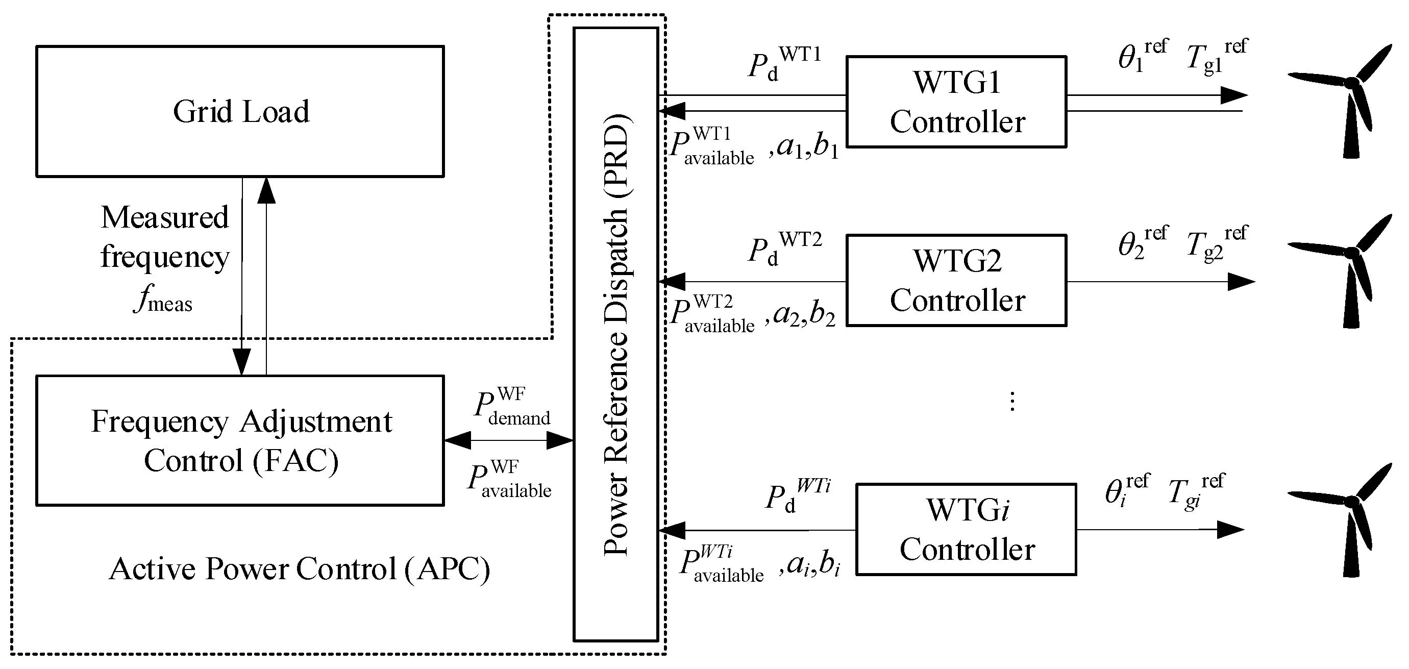
2. Control Structure of WF Participates in Frequency Regulation
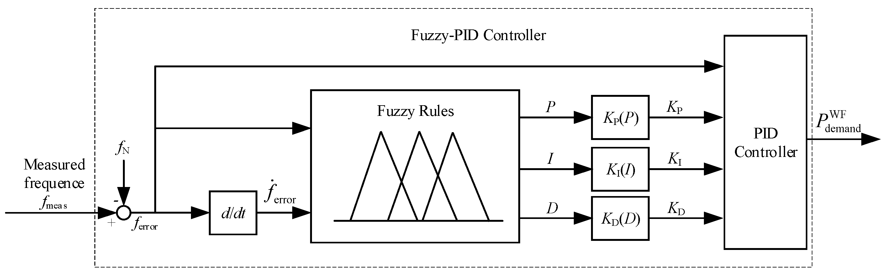
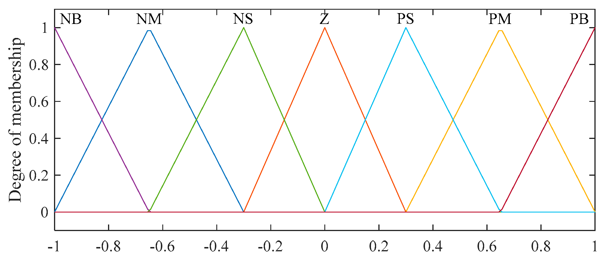
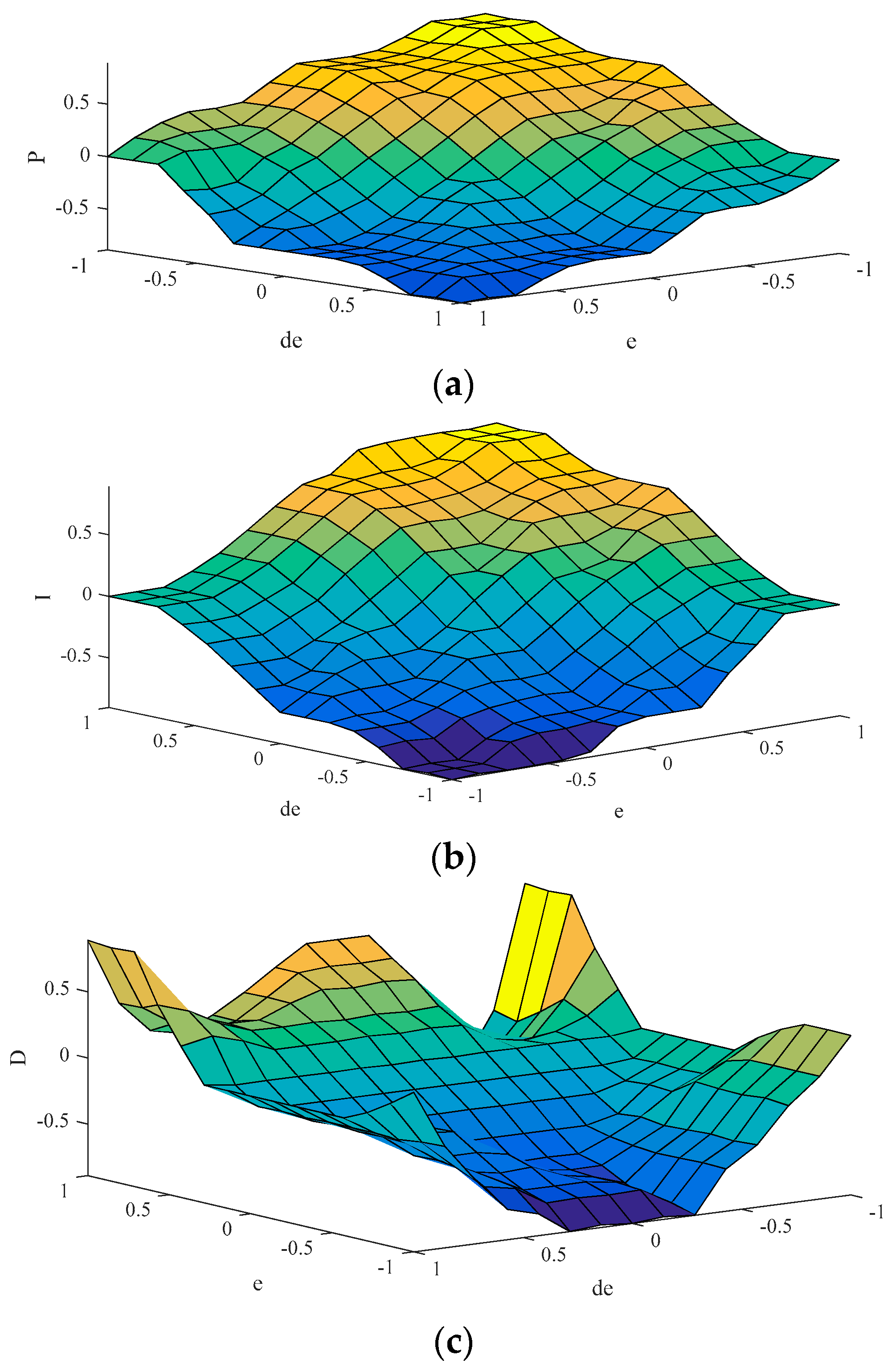
3. Fuzzy-PID Control Method of Supporting Grid Frequency Regulation for WF
4. PRD Method for WT Based on Fatigue Load Sensitivity Using Quadratic Programming Algorithm
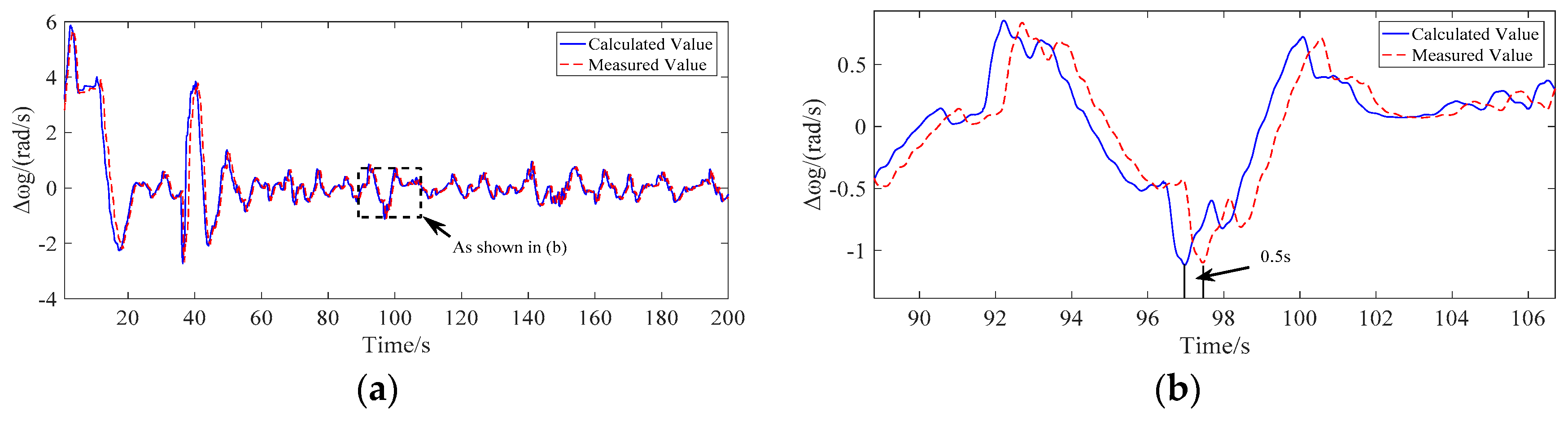
4.1. Improved Model of Fatigue Load Sensitivity
4.2. Cost Function and Constraints
5. Case Study
5.1. System Setup
5.2. Wind Farm Controller Performance
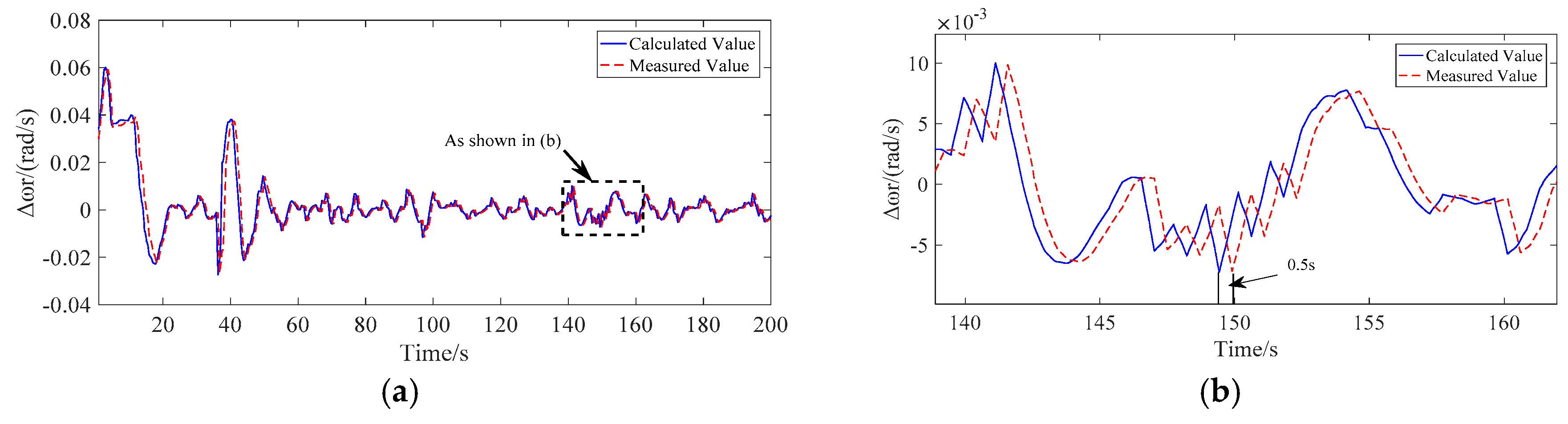
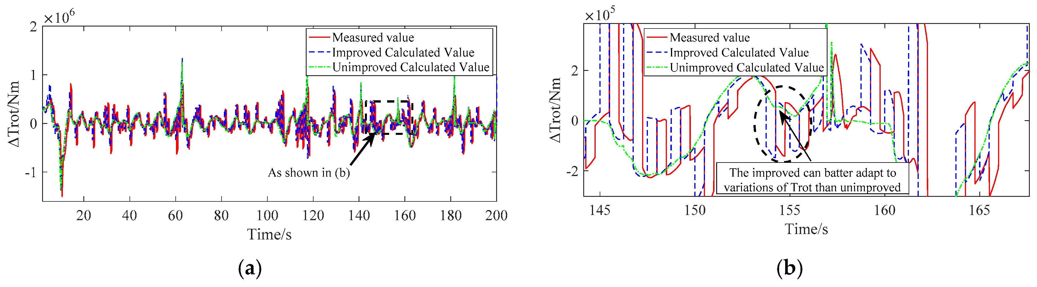
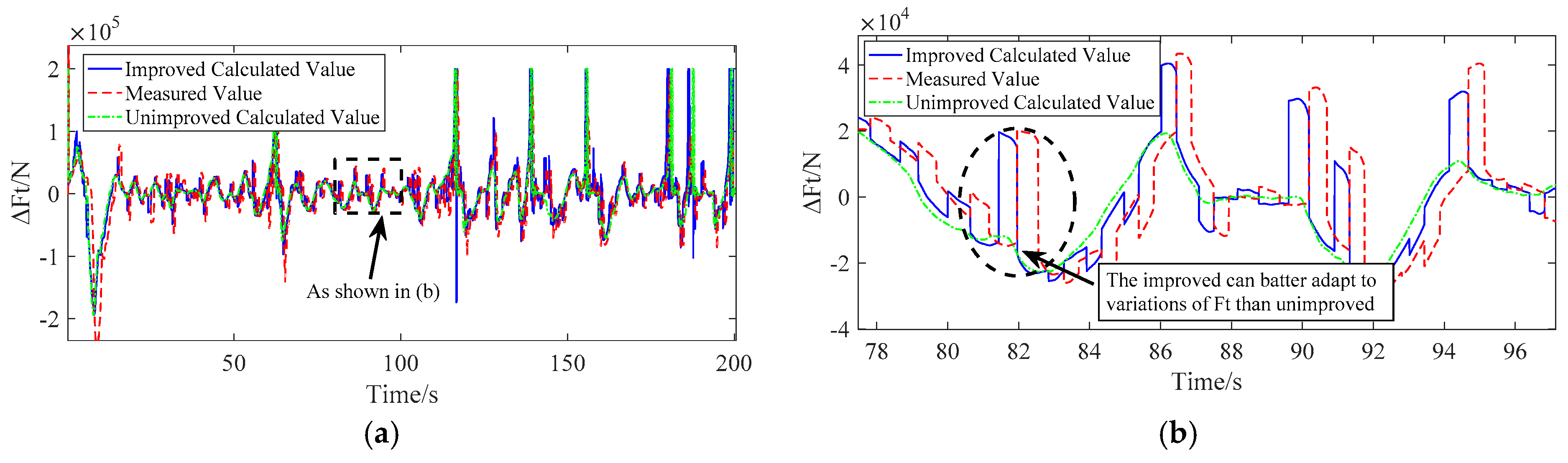
5.2.1. Performance for the Improved Model of Fatigue Load Sensitivity
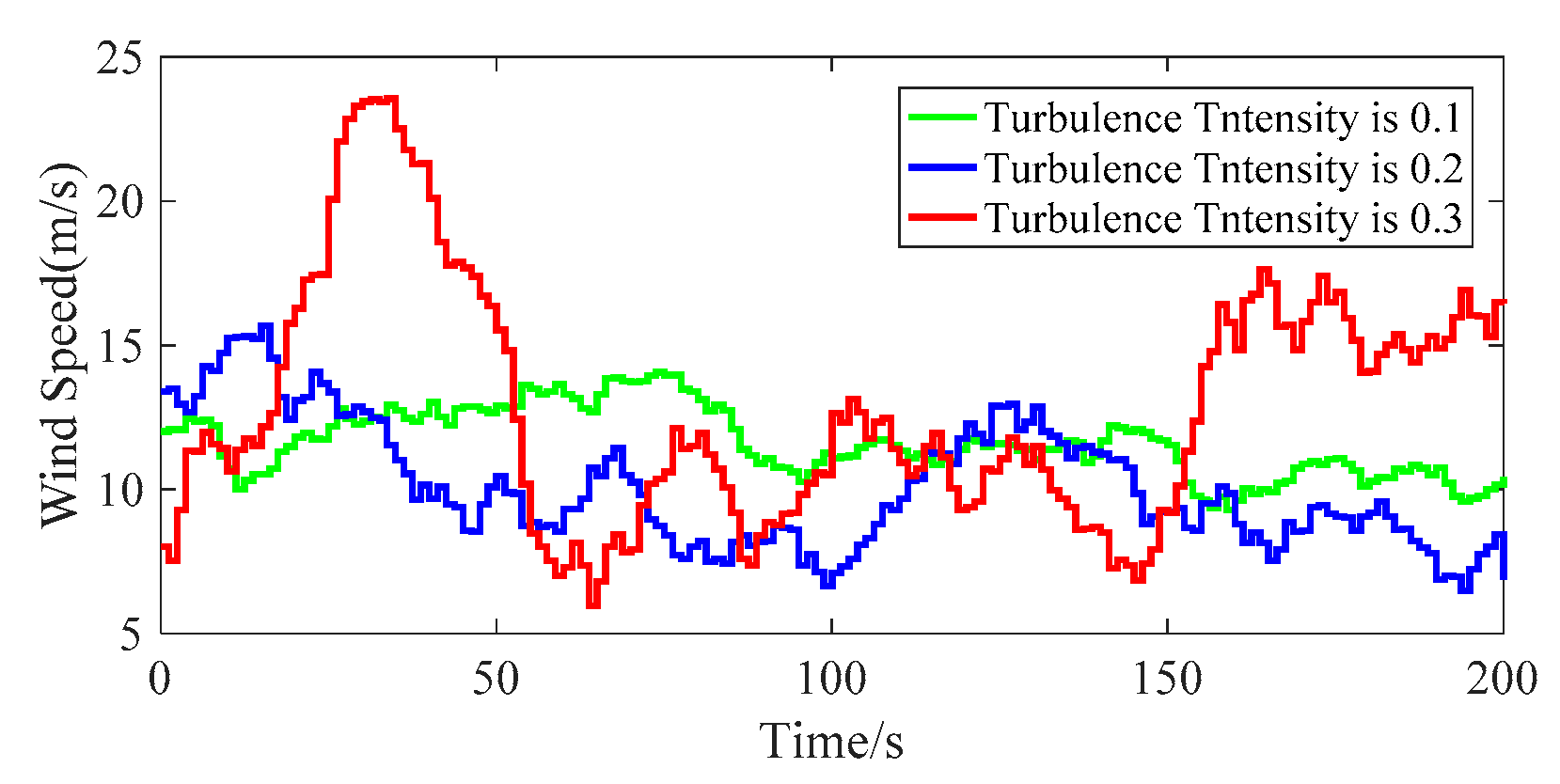
5.2.2. Performance for Different Turbulence Intensity
5.3. Overall Performance
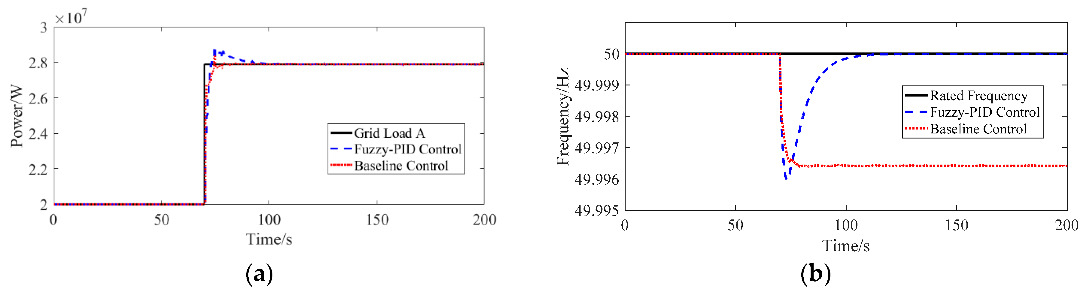
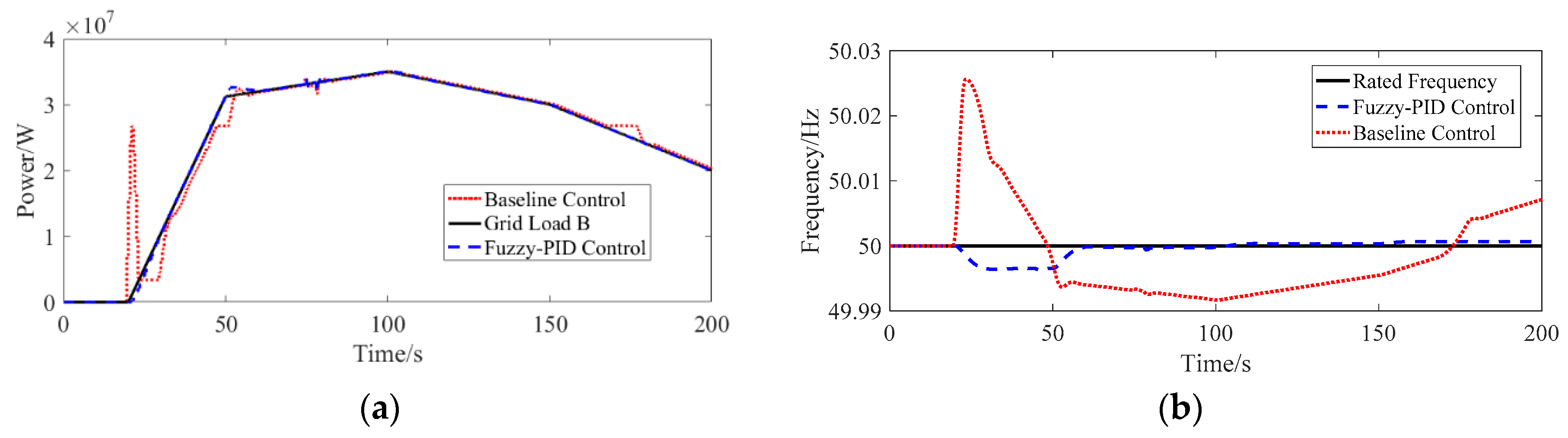
5.3.1. WF Controller Performance
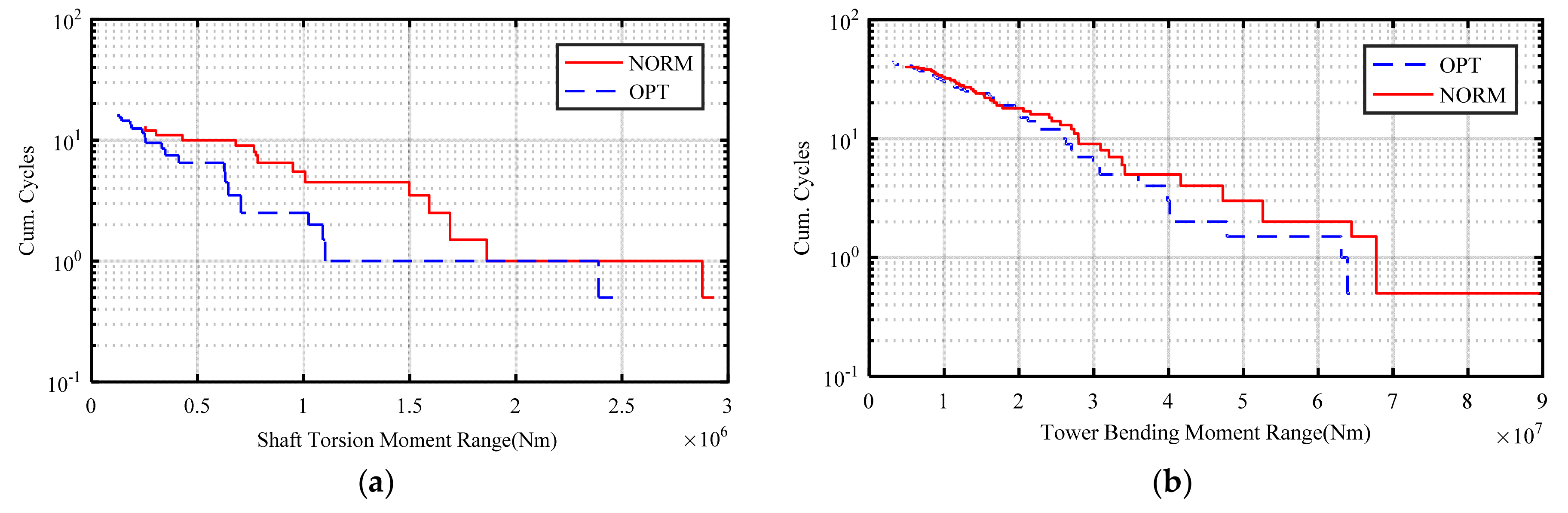
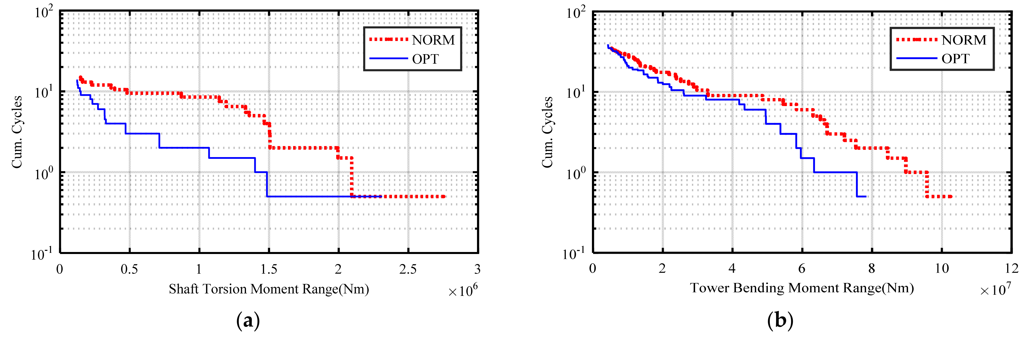
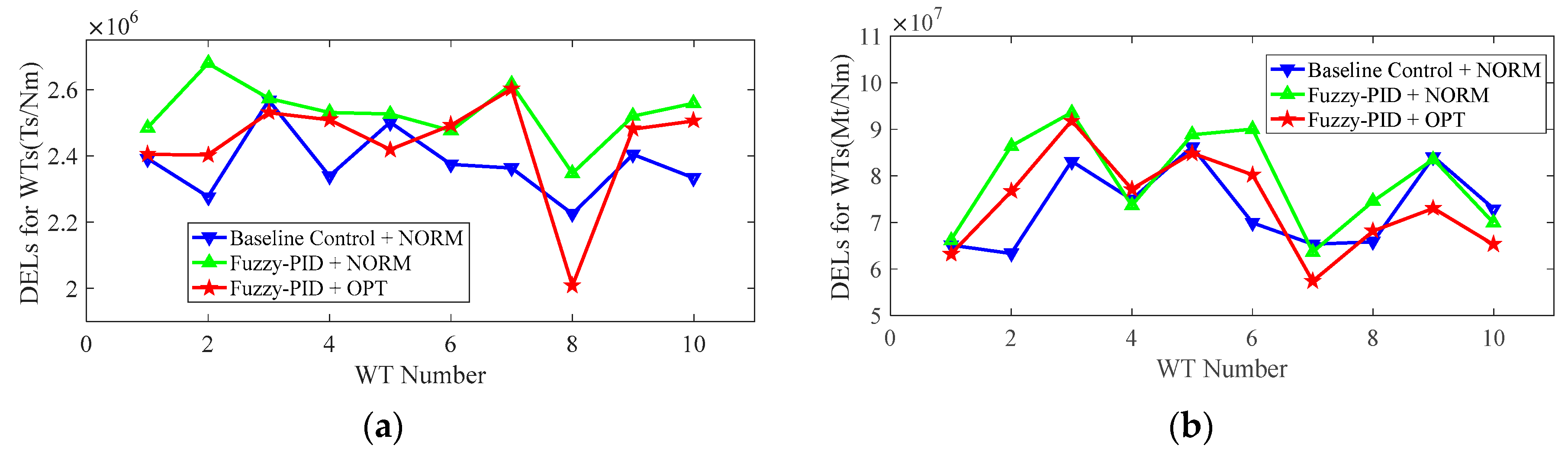
5.3.2. Fatigue Loads Performance
6. Conclusions
Author Contributions
Funding
Conflicts of Interest
Nomenclature
| Symbols | |
| KP, KI, KD | Calculated by Fuzzy-PID controller |
| bP, bI, bD | Parameters of conventional PID controller |
| aP, aI, aD | Parameters of determined the relevant ranges of variations for bP, bI, and bD |
| P, I, D | Calculated by Fuzzy Rules |
| Demanded power of wind farm | |
| Available power of wind farm | |
| Available power of wind turbine i | |
| Rated power of wind farm | |
| Reference power of wind turbine i | |
| Sensitivity of fatigue load with respect to demanded power of wind turbine | |
| Sensitivity of drive train fatigue load with respect to demanded power of wind turbine | |
| Sensitivity of the tower structural fatigue load with respect to demanded power of wind turbine | |
| Grid frequency error | |
| Grid measured frequency | |
| Normal frequency of the grid | |
| Jt | Equivalent mass of the drive-train |
| Jr | Rotational inertia of the rotor |
| Jg | Rotational inertia of the generator |
| ηg | Gear box ratio |
| ωr | Measured rotor speed |
| ωg | Measured generator speed |
| ωg-rated | Rated generator speed |
| Ft | Thrust force |
| Trot | Aerodynamic torque |
| Tg | Generator torque |
| Tg_ref | Generator torque reference |
| Ts | Shaft torque |
| Mt | Tower basefore-aft bending moment |
| Tgiref | Generator torque of wind turbine i |
| ωf | Generator filtered speed |
| τf | Time constant of the filter of ωg |
| τg | Time constant of the filter of Tg_ref |
| θiref | Pitch angle reference of wind turbine i |
| θref | Pitch angle reference of blades |
| ka, β | Functions of θref |
| kp, ki | Proportional and integral gain of θref |
| ka1, ka2 | Constants of ka |
| B | Main shaft viscous friction coefficient |
| Pg0 | Output power of a turbine at t = k |
| ωg0 | Generator speed at t = k |
| ωf0 | Filtered speed of the generator speed at t = k |
| θ0 | Pitch angle at t = k |
| Trot0 | Aerodynamic torque at t = k |
| Tg | Generator torque at t = k |
| R | Length of the blade |
| H | Tower height |
| ρ | Air density |
| v | Wind speed of hub height |
| Cp | Power coefficient |
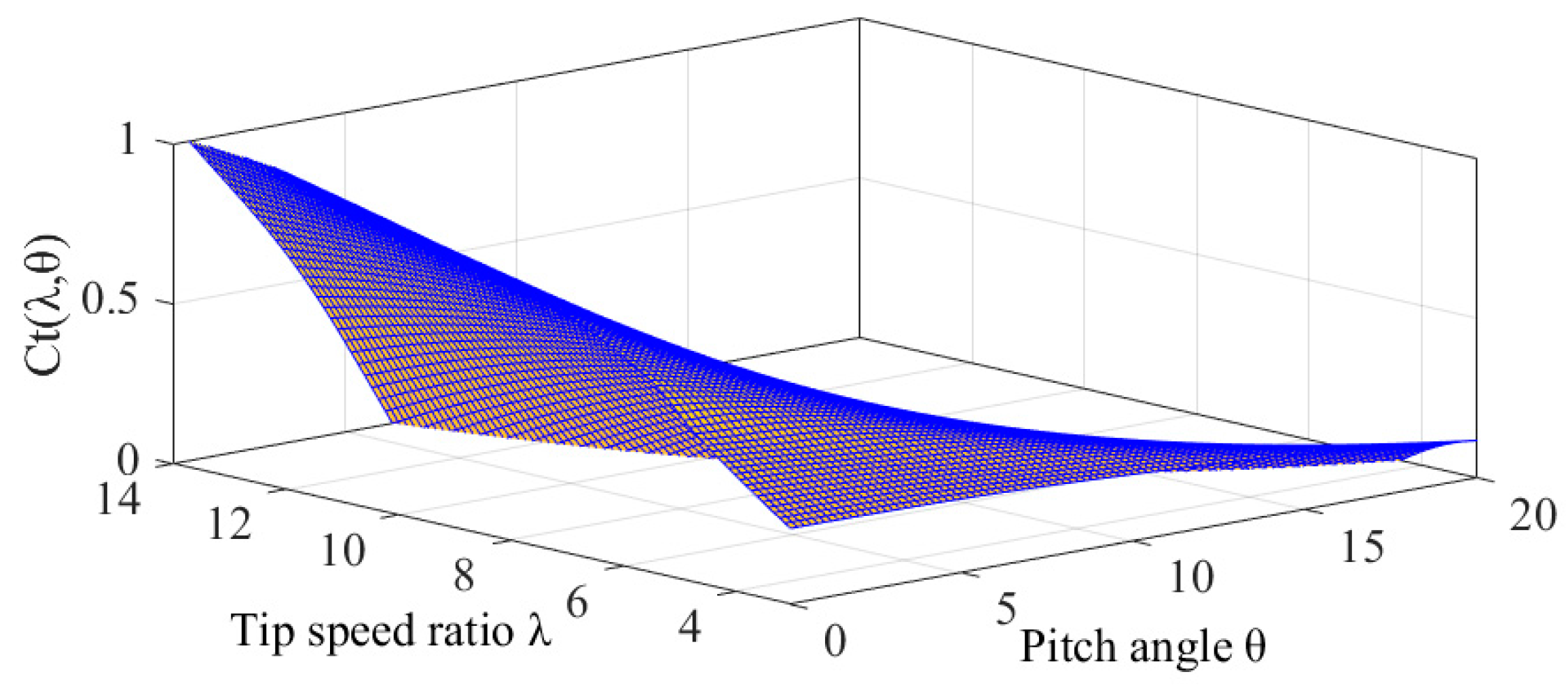
| Ct | Thrust coefficient |
| λ | Tip speed ratio |
Appendix A

References
- Sun, X.J.; Huang, D.G. An Explosive Growth of Wind Power in China. Int. J. Green. Energy 2014, 14, 849–860. [Google Scholar] [CrossRef]
- Nguyen, C.-K.; Nguyen, T.-T.; Yoo, H.-J.; Kim, H.-M. Consensus-Based SOC Balancing of Battery Energy Storage Systems in Wind Farm. Energies 2018, 11, 3507. [Google Scholar] [CrossRef]
- Bottiglione, F.; Mantriota, G.; Valle, M. Power-Split Hydrostatic Transmissions for Wind Energy Systems. Energies 2018, 11, 3369. [Google Scholar] [CrossRef]
- Kazda, J.; Cutululis, N.A. Fast Control-Oriented Dynamic Linear Model of Wind Farm Flow and Operation. Energies 2018, 11, 3346. [Google Scholar] [CrossRef]
- Wind Power Capacity Reaches 539 GW, 52,6 GW Added in 2017. 12 February 2018. Available online: http://wwindea.org/blog/2018/02/12/2017-statistics/ (accessed on 20 April 2019).
- Sun, B.; Tang, Y.; Ye, L.; Chen, C.; Zhang, C.; Zhong, W. A Frequency Control Method Considering Large Scale Wind Power Cluster Integration Based on Distributed Model Predictive Control. Energies 2018, 11, 1600. [Google Scholar] [CrossRef]
- Hou, T.T.; Lou, S.H.; Wu, Y.W. Capacity Optimization of Thermal Units Transmitted with Wind Power: A Case Study of Jiuquan Wind Power Base, China. J. Wind. Eng. Ind. Aerod. 2014, 129, 64–68. [Google Scholar] [CrossRef]
- Dai, X.M.; Zhang, K.F.; Geng, J. Study on Variability Smoothing Benefits of Wind Farm Cluster. Turk. J. Electr. Eng. Comput. Sci. 2018, 26, 1894–1908. [Google Scholar] [CrossRef]
- Du, W.J.; Bi, J.T.; Wang, T.; Hua, W. Impact of Grid Connection of Large-Scale Wind Farms on Power System Small-Signal Angular Stability. CSEE JPES 2015, 1, 83–89. [Google Scholar] [CrossRef]
- Li, J.; Ye, L.; Zeng, Y.; Wang, H.F. A Scenario-Based Robust Transmission Network Expansion Planning Method for Consideration of Wind Power Uncertainties. CSEE JPES 2016, 2, 11–18. [Google Scholar] [CrossRef]
- Liao, S.Y.; Xu, J.; Sun, Y.Z.; Bao, Y.; Tang, B.W. Wide-Area Measurement System-Based Online Calculation Method of PV Systems De-loaded Margin for Frequency Regulation in Isolated Power Systems. IET Renew. Power. Gen. 2018, 12, 335–341. [Google Scholar] [CrossRef]
- Athari, M.H.; Wang, Z. Impacts of Wind Power Uncertainty on Grid Vulnerability to Cascading Overload Failures. IEEE Trans. Sustain. Energy 2018, 9, 128–137. [Google Scholar] [CrossRef]
- You, R.; Barahona, B.; Chai, J.Y.; Cutululis, N.A.; Wu, X.Z. Improvement of Grid Frequency Dynamic Characteristic with Novel Wind Turbine Based on Electromagnetic Coupler. Renew. Energy 2017, 113, 813–821. [Google Scholar] [CrossRef]
- Oest, J.; Lund, E. Topology Optimization with Finite-life Fatigue Constraints. Struct. Multidiscip. Optim. 2017, 56, 1045–1059. [Google Scholar] [CrossRef]
- Attya, A.B.; Domínguez-García, J.L.; Bianchi, F.D.; Anaya-Lara, O. Enhancing Frequency Stability by Integrating Non-conventional Power Sources Through Multi-terminal HVDC Grid. Int. J. Electr. Power Energy Syst. 2018, 95, 128–136. [Google Scholar] [CrossRef]
- Dijk, M.T.V.; Wingerden, J.W.V.; Ashuri, T.; Li, Y. Wind Farm Multi-Objective Wake Redirection for Optimizing Power Production and Loads. Energy 2017, 121, 561–569. [Google Scholar] [CrossRef]
- Soleimanzadeh, M.; Wisniewski, R. Controller Design for a Wind Farm, Considering Both Power and Load Aspects. Mechatronics 2011, 21, 720–727. [Google Scholar] [CrossRef]
- Njiri, J.G.; Beganovic, N.; Do, M.H.; Soffker, D. Consideration of Lifetime and Fatigue Load in Wind Turbine Control. Renew. Energy 2018, 131, 818–828. [Google Scholar] [CrossRef]
- Kanev, S.K.; Savenije, F.J.; Engels, W.P. Active Wake Control: An Approach to Optimize the Lifetime Operation of Wind Farms. Wind Energy 2018, 21, 488–501. [Google Scholar] [CrossRef]
- Madani, S.M.; Akbari, M. Analytical Evaluation of Control Strategies for Participation of Doubly Fed Induction Generator-Based Wind Farms in Power System Short-Term Frequency Regulation. IET Renew. Power Gen. 2014, 8, 324–333. [Google Scholar]
- Leon, A.E.; Mauricio, J.M.; Gomezexposito, A.; Solsona, J.A. Hierarchical Wide-Area Control of Power Systems Including Wind Farms and Facts for Short-Term Frequency Regulation. IEEE Trans. Power Syst. 2012, 27, 2084–2092. [Google Scholar] [CrossRef]
- Ye, H.; Pei, W.; Qi, Z. Analytical Modeling of Inertial and Droop Responses from a Wind Farm for Short-Term Frequency Regulation in Power Systems. IEEE Trans. Power Syst. 2015, 31, 3414–3423. [Google Scholar] [CrossRef]
- Wang, Z.; Wu, W. Coordinated Control Method for DFIG-Based Wind Farm to Provide Primary Frequency Regulation Service. IEEE Trans. Power Syst. 2017, 33, 3644–3659. [Google Scholar] [CrossRef]
- Gao, Y.; Ai, Q. Distributed Multi-agent Control for Combined AC/DC Grids With Wind Power Plant Clusters. IET Gener. Transm. Dis. 2018, 12, 670–677. [Google Scholar] [CrossRef]
- Gao, X.D.; Meng, K.; Dong, Z.Y. Cooperation-Driven Distributed Control Method for Large-Scale Wind Farm Active Power Regulation. IEEE Trans. Energy Convers. 2017, 32, 1240–1250. [Google Scholar] [CrossRef]
- Badihi, H.; Zhang, Y.; Hong, H. Active Power Control Design for Supporting Grid Frequency Regulation in Wind Farms. Annu. Rev. Control. 2015, 40, 70–81. [Google Scholar] [CrossRef]
- Knudsen, T.; Bak, T.; Svenstrup, M. Survey of Wind Farm Control-Power and Fatigue Optimization. Wind Energy 2015, 18, 1333–1351. [Google Scholar] [CrossRef]
- Zhao, H.R.; Wu, Q.W.; Guo, Q.; Sun, H.B.; Xue, Y.S. Distributed Model Predictive Control of a Wind Farm for Optimal Active Power Control—Part II: Implementation with Clustering-Based Piece-Wise Affine Wind Turbine Model. IEEE Trans. Sustain. Energy 2015, 6, 840–849. [Google Scholar] [CrossRef]
- Zhao, H.R.; Wu, Q.W.; Guo, Q.; Sun, H.B.; Xue, Y.S. Optimal Active Power Control of a Wind Farm Equipped with Energy Storage System Based on Distributed Model Predictive Control. IET Gener. Transm. Distrib. 2016, 10, 669–677. [Google Scholar] [CrossRef]
- Zhao, H.R.; Wu, Q.W.; Huang, S.J.; Shahidehpour, M.; Guo, Q.; Sun, H.B. Fatigue Load Sensitivity Based Optimal Active Power Dispatch for Wind Farms. IEEE Trans. Sustain. Energy 2017, 8, 1247–1259. [Google Scholar] [CrossRef]
- Yuan, S.; Zhao, C.; Guo, L. Uncoupled PID Control of Coupled Multi-Agent Nonlinear Uncertain Systems. J. Syst. Sci. Complex. 2018, 31, 4–21. [Google Scholar] [CrossRef]
- Zhang, M.; Rosales, L.P.B.; Ortega, R.; Liu, Z.; Su, H. Pid, Passivity-Based Control of Port-Hamiltonian Systems. IEEE Trans. Autom. Control 2018, 63, 1032–1044. [Google Scholar] [CrossRef]
- Mahto, T.; Mukherjee, V. Fractional Order Fuzzy PID Controller for Wind Energy-Based Hybrid Power System Using Quasi-Oppositional Harmony Search Algorithm. IET Gener. Transm. Dis. 2017, 11, 3299–3309. [Google Scholar] [CrossRef]
- Gil, P.; Sebastião, A.; Lucena, C. Constrained Nonlinear-Based Optimisation Applied to Fuzzy PID Controllers Tuning. Asian J. Control 2018, 20, 135–148. [Google Scholar] [CrossRef]
- Amirhossein, A.; Reza, S.; Ali, J. Performance and Robustness of Optimal Fractional Fuzzy PID Controllers for Pitch Control of a Wind Turbine Using Chaotic Optimization Algorithms. ISA Trans. 2018, 79, 27–44. [Google Scholar]
- Mohan, V.; Chhabra, H.; Rani, A.; Singh, V. An Expert 2DOF Fractional Order Fuzzy PID Controller for Nonlinear Systems. Neural Comput. Appl. 2018, 1–18. [Google Scholar] [CrossRef]
- Vedrana, S.; Mate, J.; Baotić, M. Wind Turbine Power References in Coordinated Control of Wind Farms. Autom. J. Control Meas. Electron. Comput. Commun. 2011, 52, 82–94. [Google Scholar]
- Barlas, T.K.; Kuik, G.A.M.V. Review of State of the Art in Smart Rotor Control Research for Wind Turbines. Prog. Aerosp. Sci. 2010, 46, 1–27. [Google Scholar] [CrossRef]
- Jonkman, J.M.; Butterfield, S.; Musial, W.; Scott, G. Definition of a 5-MW Reference Wind Turbine for Offshore System Development; National Renewable Energy Lab.: Lakewood, CO, USA, 2009. [Google Scholar]
- Grunnet, J.D.; Soltani, M.; Knudsen, T.; Kragelund, M.N.; Bak, T. Aeolus Toolbox for Dynamic Wind Farm Model, Simulation and Control. In Proceedings of the European Wind Energy Conference & Exhibition, Warsaw, Poland, 20–23 April 2010. [Google Scholar]
- Pardalos, P.M.; Rebennack, S.; Pereira, M.V.F.; Iliadis, N.A.; Pappu, V. Handbook of Wind Power Systems; Springer: Berlin, Germany, 2014. [Google Scholar]
- Soltani, M.N.; Knudsen, T.; Svenstrup, M.; Wisniewski, R.; Brath, P.; Ortega, R.; Johnson, K. Estimation of Rotor Effective Wind Speed: A Comparison. IEEE Trans. Control Syst. Technol. 2013, 21, 1155–1167. [Google Scholar] [CrossRef]
- Manwell, J.F.; Mcgowan, J.G.; Rogers, A.L. Wind Energy Explained: Theory, Design and Application, 2nd ed.; John Wiley & Sons: Hoboken, NJ, USA, 2002. [Google Scholar]
- Simley, E.; Dunne, F.; Laks, J.; Pao, L.Y. 10 Lidars and Wind Turbine Control—Part 2. DTU Wind Energy-E-Report-0029. Available online: http://citeseerx.ist.psu.edu/viewdoc/download;jsessionid=16F5DC8769E46EEC0A5834631C48C1E0?doi=10.1.1.361.2830&rep=rep1&type=pdf (accessed on 21 April 2019).
- Luis, V.; Salvador, J. Quadratic programming. J. Oper. Res. Soc. 2013, 16, 256–257. [Google Scholar]
- Cimini, G.; Bemporad, A. Exact Complexity Certification of Active-Set Methods for Quadratic Programming. IEEE Trans. Autom. Control. 2017, 62, 6094–6109. [Google Scholar] [CrossRef]
- Bao, Y.; Xiong, T.; Hu, Z. PSO-MISMO Modeling Strategy for Multistep-Ahead Time Series Prediction. IEEE Trans. Cybern. 2014, 44, 655–668. [Google Scholar] [PubMed]
- Nery, G.A., Jr.; Martins Márcio, A.F.; Kalid, R. A PSO-Based Optimal Tuning Strategy for Constrained Multivariable Predictive Controllers with Model Uncertainty. ISA Trans. 2014, 53, 560–567. [Google Scholar] [CrossRef]
- Sahu, R.K.; Panda, S.; Chandra Sekhar, G.T. A Novel Hybrid PSO-PS Optimized Fuzzy PI Controller for AGC in Multi Area Interconnected Power Systems. Int. J. Elec. Power 2015, 64, 880–893. [Google Scholar] [CrossRef]
- Gong, D.W.; Sun, J.; Miao, Z. A Set-Based Genetic Algorithm for Interval Many-Objective Optimization Problems. IEEE Trans. Evol. Comput. 2016, 22, 47–60. [Google Scholar] [CrossRef]
- Buhl, M. MCrunch User’s Guide for Version 1.00, 1st ed.; National Renewable Energy Laboratory: Lakewood, CO, USA, 2008. [Google Scholar]


| Linguistic Variables | Meaning |
|---|---|
| NB | Negative big |
| NM | Negative medium |
| NS | Negative small |
| Z | Zero |
| PS | Positive small |
| PM | Positive medium |
| PB | Positive big |
| λ | λmin | λmin + Δλ | … | λmax | |
|---|---|---|---|---|---|
| θ | |||||
| θmin | 0.0005 | 0.001 | … | −0.8478 | |
| θmin + Δθ | 0.0005 | 0.001 | … | −0.8637 | |
| … | … | … | … | … | |
| θmax | −0.0012 | −0.0036 | … | −207.6793 | |
| Parameter | Value |
|---|---|
| fN | 50 Hz |
| aP | 1 × 10⁸ |
| bP | 3 × 10⁸ |
| aI | 5 × 10⁶ |
| bI | 5 × 10⁷ |
| aD | 5 × 10⁷ |
| bD | 2 × 10⁸ |
| Parameter | Value |
|---|---|
| Rotor inertia: Jr | 3.54 × 10⁷ (kg∙m2) |
| Generator inertia: Jg | 5.34 × 10² (kg∙m2) |
| Gear box ratio: ηg | 97 |
| Filter time constant of ωg: τf | 10 |
| Proportional gain: kp | 0.2143 |
| Integral gain: ki | 0.0918 |
| Gain coefficient: ka1 | 2.1323 |
| Gain coefficient: ka2 | 1 |
| Generator rated speed: ωg-rated | 122.91 (rad/s) |
| Main shaft viscous friction coefficient: B | 6.22 × 10⁶ (Nm∙s/rad) |
| Sir density: ρ | 1.22 (kg/m3) |
| Length of the blade: R | 63 (m) |
| Filter time constant of Tg_ref: τg | 0.1 |
| No. | DELs for WTs (Ts/MNm) | DELs for WTs (Mt/MNm) | ||||
|---|---|---|---|---|---|---|
| NORM | OPT | Percentage | NORM | OPT | Percentage | |
| 1 | 1.94 | 2.06 | 6.13% | 50.48 | 44.96 | −10.93% |
| 2 | 1.94 | 1.76 | −9.38% | 57.48 | 57.92 | 0.77% |
| 3 | 1.82 | 1.77 | −2.26% | 62.68 | 60.90 | −2.83% |
| 4 | 1.82 | 1.70 | −6.73% | 54.19 | 47.86 | −11.68% |
| 5 | 1.85 | 2.28 | 23.39% | 42.83 | 40.86 | −4.59% |
| 6 | 1.86 | 1.66 | −11.04% | 59.97 | 58.95 | −1.71% |
| 7 | 1.74 | 1.55 | −10.86% | 65.75 | 64.67 | −1.64% |
| 8 | 1.83 | 1.45 | −20.89% | 48.69 | 40.87 | −16.05% |
| 9 | 1.87 | 2.08 | 11.01% | 42.00 | 38.29 | −8.83% |
| 10 | 1.80 | 1.76 | −2.48% | 58.64 | 58.56 | −0.15% |
| summary | 18.47 | 18.07 | −2.21% | 542.76 | 513.90 | −5.32% |
| Turbulence Intensity | DELs for WTs (Ts/MNm) | DELs for WTs (Mt/MNm) | ||||
|---|---|---|---|---|---|---|
| NORM | OPT | Percentage | NORM | OPT | Percentage | |
| 0.2 | 15.78 | 14.97 | −5.13% | 616.40 | 577.77 | −6.28% |
| 0.3 | 14.63 | 14.27 | −2.46% | 646.93 | 611.33 | −5.50% |
| Control Method | NRMSE for Power Responses | SD for grid Frequency Responses | ||
|---|---|---|---|---|
| Grid Load A | Grid Load B | Grid Load A | Grid Load B | |
| Baseline Control | 0.017545 | 0.104380 | 0.002845 | 0.007423 |
| Fuzzy-PID | 0.021409 | 0.012052 | 0.000764 | 0.001345 |
| DELs for WTs (Mt/MNm) | DELs for WTs (Ts/MNm) | |||
|---|---|---|---|---|
| Values | Percentage | Values | Percentage | |
| Baseline Control + NORM | 730.68 | 23.77 | ||
| Fuzzy-PID + NORM | 790.23 | 8.15% | 25.31 | 6.47% |
| Fuzzy-PID + OPT | 733.01 | 0.32% | 24.35 | 2.44% |
© 2019 by the authors. Licensee MDPI, Basel, Switzerland. This article is an open access article distributed under the terms and conditions of the Creative Commons Attribution (CC BY) license (http://creativecommons.org/licenses/by/4.0/).
Share and Cite
Liu, Y.; Wang, Y.; Wang, X.; Zhu, J.; Lio, W.H. Active Power Dispatch for Supporting Grid Frequency Regulation in Wind Farms Considering Fatigue Load. Energies 2019, 12, 1508. https://doi.org/10.3390/en12081508
Liu Y, Wang Y, Wang X, Zhu J, Lio WH. Active Power Dispatch for Supporting Grid Frequency Regulation in Wind Farms Considering Fatigue Load. Energies. 2019; 12(8):1508. https://doi.org/10.3390/en12081508
Chicago/Turabian StyleLiu, Yingming, Yingwei Wang, Xiaodong Wang, Jiangsheng Zhu, and Wai Hou Lio. 2019. "Active Power Dispatch for Supporting Grid Frequency Regulation in Wind Farms Considering Fatigue Load" Energies 12, no. 8: 1508. https://doi.org/10.3390/en12081508
APA StyleLiu, Y., Wang, Y., Wang, X., Zhu, J., & Lio, W. H. (2019). Active Power Dispatch for Supporting Grid Frequency Regulation in Wind Farms Considering Fatigue Load. Energies, 12(8), 1508. https://doi.org/10.3390/en12081508