An Injectivity Evaluation Model of Polymer Flooding in Offshore Multilayer Reservoir

1
Research Institute of Petroleum Exploration & Development, PetroChina, Beijing 100083, China
2
Key Laboratory of Petroleum Engineering of the Ministry of Education, China University of Petroleum, Beijing 102249, China
*
Author to whom correspondence should be addressed.
Energies 2019, 12(8), 1444; https://doi.org/10.3390/en12081444
Submission received: 9 March 2019
/
Revised: 1 April 2019
/
Accepted: 9 April 2019
/
Published: 15 April 2019
(This article belongs to the Special Issue Enhanced Oil Recovery 2019)
Abstract
:Good polymer flood performance evaluation requires an understanding of polymer injectivity. Offshore reservoirs are characterized by unfavorable water–oil mobility ratios, strong heterogeneity, and multilayer production, which collectively contribute to unique challenges. Accordingly, this article presents a semi-analytical model for the evaluation of commingled and zonal injectivity in the entire development phase, which consists of primary water flooding, secondary polymer flooding, and subsequent water flooding. First, we define four flow regions with unique saturation profiles in order to accurately describe the fluid dynamic characteristics between the injector and the producer. Second, the frontal advance equation of polymer flooding is built up based on the theory of polymer–oil fractional flow. The fluid saturation distribution and the injection–production pressure difference are determined with the method of equivalent seepage resistance. Then, the zonal flow rate is obtained by considering the interlayer heterogeneity, and the semi-analytical model for calculating polymer injectivity in a multilayer reservoir is established. The laboratory experiment data verify the reliability of the proposed model. The results indicate the following. (1) The commingled injectivity decreases significantly before polymer breakthrough and increases steadily after polymer breakthrough. The change law of zonal injectivity is consistent with that of commingled injectivity. Due to the influence of interlayer heterogeneity, the quantitative indexes of the zonal flow rate and injection performance are different. The injectivity of the high-permeability layer is better than that of the low-permeability layer. (2) The higher the injection rate and the lower the polymer concentration, the better the injectivity is before polymer breakthrough. An earlier injection time, lower injection rate, larger polymer injection volume, and lower polymer concentration will improve the injectivity after polymer breakthrough. The polymer breakthrough time is a significant indicator in polymer flooding optimization. This study has provided a quick and reasonable model of injectivity evaluation for offshore multilayer reservoirs.
1. Introduction
Polymer flooding is of considerable interest for its application in the development of mature oilfields. In recent years, stimulated by the success of polymer flooding for increasing oil and controlling water in onshore oilfields, explorations and practices of polymer flooding have been conducted in some offshore oilfields [1,2,3,4]. One important factor for evaluating the applicability of polymer flooding is polymer injectivity in reservoir conditions [5]. However, the accurate evaluation of polymer injectivity has been regarded as one of the key technical difficulties that could be encountered for the successful implementation of polymer flooding. Especially for offshore reservoirs with characteristics such as a thick pay zone, multilayer, viscous oil, commingled production, and large well spacing [6], polymer injectivity ties to polymer solution rheology, polymer–oil seepage resistance, and interlayer heterogeneity.
In situ non-Newtonian polymer rheology is the most crucial factor that affects polymer injectivity. During the early polymer flooding in the Bohai offshore oilfield, hydrophobically associative polymer solution (HAPS) has been widely applied owing to its fine quality of temperature resistance, salt resistance, and shear resistance, which can help the solution keep a high viscosity at a high injection rate and a high salinity [7,8,9,10]. Studies have shown that polymer concentration and reservoir heterogeneity can influence the displacement effect of polymer flooding. Moreover, affected by the sedimentary environment and the exploitation mode of enhanced injection and production in offshore oilfields, the interlayer heterogeneity increases and the physical properties between the high-permeability layer and the low-permeability layer differ greatly [11]. Xie [12] performed a polymer flooding experiment of parallel cores, and demonstrated that compatibility exists between HAPS molecular aggregation and pore-throat size. The applicability for a heterogeneous reservoir can be influenced by polymer concentration. Accordingly, it is required to make further analysis of HAPS injectivity for multilayer reservoirs.
Several mathematical models have been developed to assess polymer injectivity with an emphasis on fractional flow theory and phase behavior. Lake [13] first defined the injectivity of a well as the ratio of the volumetric injection rate to the pressure drop, and proposed a one-dimensional, steady-state, radial flow model for analyzing single-well injectivity. Seright [14] investigated the influence of mechanical degration and viscoelasticity on the polymer injectivity during radial core flood by separating the injection pressure drop into four components, including the entrance pressure drop associated with polymer mechanical degradation at the sandface, the pressure drop associated with dilatant or viscoelastic polymer behavior near a wellbore, the pressure drop associated with polymer solutions flowing at low fluxes and exhibiting a Newtonian or flux-independent behavior, and the pressure drop associated with the flow of brine and oil. However, the pressure drops were valid only at the early stage of polymer injection, and the injectivity performance after polymer breakthrough was difficult to predict. Shuler et al. [15] presented a monolayer radial flow model with constant-pressure boundary conditions to calculate the bottom-hole pressure during the single-well polymer injectivity test. The total pressure drop was the summation of the pressure drop of the oil-brine zone ahead of the polymer zone, the pressure drop across the polymer zone, and the pressure drop caused by skin effects. However, this model assumed the polymer flow to be piston-like displacement, and neglected the effect of polymer shear degradation in the near-wellbore. Buell [16,17] developed a two-phase, radial, numerical reservoir simulator to analyze non-Newtonian fluid injectivity by modifying the Hall plot. This method created three fluid banks that consisted of water, polymer, and oil for calculating an injection pressure drop. Since the Hall plot requires long-term injection data to achieve a smoothing effect, it is not applicable to the injectivity prediction for early-stage polymer flooding with short pre-water injection. Liu et al. [18] established the injectivity models that considered the Newtonian rheology, power law rheology, and viscoelastic rheology, and analyzed the influence of rheology on polymer injectivity. Meanwhile, the assumption that polymer flowing was a single aqueous phase did not consider the kinetic mechanism of an oil bank forming during polymer flooding, nor did it investigate the nature of polymer–oil fractional flow. Alsofi and Blunt [19,20] proposed a novel scheme based on the segregation-in-flow assumption to better resolve saturation fronts in streamline-based simulations of polymer flooding, but this scheme might not apply to cases in which different concentrations are injected through time or in different locations.
In view of the vertical heterogeneity of an offshore multilayer reservoir, the zonal injectivity performance and fluid dynamic characteristics also have to be considered in order to investigate the impact of non-Newtonian behavior on the injection profile and conformance efficiency. Jain and Lake [21] introduced an analytical model of volumetric sweep in a two-dimensional (2D) layered reservoir that aimed to apply an extension of Koval’s theory [22] where flow was assumed to be segregated under vertical equilibrium conditions for polymer displacement. The segregated flow was represented as two fronts that separated the oil bank region from the region that contained injected solvent and water, and the remaining oil region from the secondary flood and water. Seright [23] presented a base-case method for deciding the optimal polymer viscosity injected to a layered reservoir. He also pointed out that in a layered reservoir, injecting polymer solutions enforced cross flow between layers with different properties, which accelerated the oil displacement in low-permeability layers. Luo [24] developed an implicit well-rate allocation model to accurately allocate the injection rate into different layers with contrasting permeabilities. Lu [25] defined several flow regions with unique saturation profiles during polymer flooding, and then established a semi-analytical model for predicting multilayer injection capacity. This model properly described the oil saturation distribution near a wellbore, instead of treating the underground fluid as a pure polymer solution, and took into account the water–oil flow function. Despite the current efforts made by using analytical or semi-analytical solutions to clarify the injectivity characteristics during polymer flooding, there is lack of complete understanding of the mechanisms behind polymer–oil fractional flow during non-piston-like displacement and an in-depth analysis of commingled and zonal injectivity at different development stages.
The objective of this article is to present a concept “based on the fluid dynamic characteristics from every frontal saturation between injector and producer” by dividing the entire flow region into interrelated parts, and then apply this information to quantitatively calculate the zonal flow rate and fluid injectivity by the semi-analytical model established on the basis of polymer–oil fractional flow theory and the equivalent seepage resistance method. The main features of this methodology are that it gives an insight into the displacement performance in a given well pattern, including the near-wellbore and interwell areas, and also captures the commingled and zonal injectivity characteristics in the whole life-cycle development incorporating primary water flood, secondary polymer flood, and subsequent water flood. This proposed model is capable of considering important mechanisms influencing injectivity, and extends the laboratory results to the field scale. The findings may be beneficial in polymer screening and the designing of polymer flood for enhanced oil recovery in offshore multilayer reservoirs.
2. Physical Model and Basic Assumptions
In consideration of the limited platform space and life span of facilities (20–25 years), polymer flooding for offshore oilfields is usually conducted at the early development stage. The inverted nine-spot pattern or inverted seven-spot pattern is widely deployed that can meet the requirements of a high production rate and later-stage well pattern adjustment such as infilling or converting into a five-spot pattern [6]. As shown in Figure 1, based on the theory of fractional flow in polymer flooding, a composite flow model for polymer solution is established. The injector at the center of the well pattern in a multilayer reservoir is injected with water, polymer solution, and water successively, and the seepage regions are divided into a polymer single-phase flow region, oil bank region, water–oil two-phase flow region, and oil drainage region. The basic assumptions are made as follows:
- (1)
- The seepage medium is homogeneous, isotropic, and incompressible.
- (2)
- The displacement is non-piston like with a constant injection rate.
- (3)
- The gravity, capillary force, and fluid diffusion are negligible.
- (4)
- The constitutive equation of the polymer solution as non-Newtonian fluid follows the power-law model.
- (5)
- The polymer solution is divided into two phases: a polymer phase and an oil phase. This polymer is only soluble in water and insoluble in oil.
- (6)
- The polymer solution only reduces the relative permeability of the water phase without changing that of the oil phase.
- (7)
- The fluid flow follows the generalized Darcy’s law, and the cross flow is not considered.
3. Mathematical Model
3.1. Fluid Saturation Distribution in Polymer Flooding
According to the field application of polymer flooding in offshore oilfields, the injection of polymer solution into a high-viscosity reservoir will lead to the rapid increase of injection pressure, resulting in injectivity impairment. Since the volumetric injection rate during polymer flooding is constrained by formation fracture pressure, the project economics may be significantly affected. Thus, it is necessary that the water is pre-injected into a well for a period of time before polymer flooding to improve the polymer injectivity. Based on previous study on the optimization of polymer injection parameters in the Bohai oilfield, polymer solution should be injected before the change rate of water cut in the water-flooding phase reaches the maximum, during which the water cut ranges from 30% to 60%. This enables the mobility control and the likelihood that the polymer injection pressure will remain stable in a given application [26].
During the displacement process of oil and retained water, the retained water and polymer solution are miscible. Due to the viscosity difference, the distribution of fluid saturation is discontinuous at the fluid interface. The oil saturation will increase with time at the polymer front, and the oil enrichment region will be formed, which is called the oil bank [27]. Therefore, during the process of polymer flooding after water breakthrough, there are three flow regions between the injector and producer, namely, the polymer single-phase flow region, the oil bank region, and the water–oil two-phase flow region. Based on the fractional flow theory in polymer flooding, the frontal fluid saturation, velocity, and position of each flow region can be calculated. Thus, the overall distribution of fluid saturation between injector and producer is determined.
3.1.1. Frontal Saturation in Polymer Single-Phase Flow Region
Subject to basic assumptions, the polymer solution is only transported in the aqueous phase, which can both be treated as one phase. Under the condition of constant rate displacement, we obtain the continuity equations of the polymer component and the water component, respectively:
Equation (1) can be expressed as follows:
with:
where ϕ is the porosity, dimensionless; Sw is the water saturation, dimensionless; Cp is the concentration of polymer component in the water phase, mg/cm3; ρs is the rock density, g/cm3; Crp is the adsorption concentration of the polymer component in the rock phase, mg/cm3; v is the seepage velocity, m/s; fp is the water saturation corresponding to water cut in the polymer–oil fractional flow curve, dimensionless; q is the cumulative flow rate, m3/s; and A is the cross-section area, m2.
In combination with Equations (2) and (3), we obtain:
By solving Equation (5) with the characteristic method, the rate of frontal advance is:
with:
where ϕe is the inaccessible pore volume, dimensionless; and Dp is the polymer retardation factor, dimensionless.
Since the polymer adsorption is Langmuir-like, and because the polymer displaces the connate water miscibly, the polymer front has a specific velocity:
where is the polymer front saturation, dimensionless; and is the velocity of polymer frontal advance, m/s.
From Equation (2), we obtain:
The velocity of polymer frontal advance can also be expressed as follows:
In combination with Equations (8) and (10), will be determined by:
Equation (11) is the implicit function expression of . Similar to the approach to solving the frontal saturation in the water–oil two-phase flow, can be determined by using the graphical method. As is shown in Figure 2, on the relation curve of water cut and water saturation, a tangent line is made to the polymer–oil fractional flow curve through the point of (−Dp + ϕe, 0). Accordingly, is the water saturation corresponding to the tangential point.
3.1.2. Frontal Saturation in Oil Bank Region
When the injection rate is constant, we assume that the polymer front moves from xf (t) to xf (t + Δt) during the time interval of Δt. According to the law of conservation of matter, the variation of water cut is:
where is the frontal saturation of the oil bank, dimensionless.
Equation (12) can also be expressed as follows:
When Δt approaches zero, is given by:
Equations (8) and (14) will determine the frontal saturation of the oil bank.
Equation (15) is the implicit function expression of , which can also be solved by using the graphical method. As is shown in Figure 2, on the relation curve of water cut and water saturation, a tangent line is made to the polymer–oil fractional flow curve through the point of (−Dp + ϕe, 0). Accordingly, is the water saturation corresponding to the intersection point of the tangential line and the water–oil fractional flow curve.
3.1.3. Breakthrough Time of Displacement Front
In order to simplify the calculation, the dimensionless distance and dimensionless time are defined respectively as:
where xD is the dimensionless distance; tD is the dimensionless time; and Vp is the pore volume, m3.
According to the frontal advance equation in polymer flooding, the frontal positions of the polymer single-phase region and oil bank region are expressed as follows, respectively:
where xD1 is the frontal position of the polymer single-phase flow region, dimensionless; xD2 is the frontal position of the oil bank region, dimensionless, and is the derivative of the polymer–oil fractional flow curve.
Let xD = 1; then, the breakthrough time of the polymer front and oil bank are determined respectively as:
where tD1 is the breakthrough time of the polymer front, dimensionless; and tD2 is the breakthrough time of the oil bank, dimensionless.
Accordingly, the global distribution of fluid saturation during the process of polymer flooding is shown in Figure 3.
3.2. Pressure Difference between Injector and Producer
3.2.1. Pressure Difference between Injector and Producer in Water Flooding
The seepage resistance regions between the injector and producer before water breakthrough in water flooding are divided into four regions, including the region between the injection well bottom and the water zone front, the water–oil two-phase flow region, the region between the water–oil two-phase zone front and the oil drainage zone, and the region between the oil drainage zone and the production well bottom. According to the method of equivalent seepage resistance, the pressure difference of each region can be expressed as follows, respectively:
where Δpw1 is the pressure difference between the injection well bottom and the water zone front, MPa; Δpw2 is the pressure difference of the water–oil two-phase flow region, MPa; Δpw3 is the pressure difference between the water–oil two-phase flow front and the oil drainage zone, MPa; and Δpw4 is the pressure difference between the oil drainage zone and the production well bottom, MPa. q(t) is the injection rate, m3/s; k is the absolute permeability,10−3 µm2; h is the net pay thickness, m; is the second derivative of the water–oil fractional flow curve, dimensionless; µw is the water viscosity, mPa·s; µo is the oil viscosity, mPa·s; krw is the water-phase relative permeability, dimensionless; krw is the oil-phase relative permeability, dimensionless; Swf is the frontal saturation of the oil–water two-phase flow region, dimensionless; Swm is the maximum water saturation at the injection well bottom, dimensionless; Swc is the irreducible water saturation, dimensionless; rw is the bottom hole radius, m; rw1 is the distance between the injection well bottom and the water zone front, m; rw2 is the distance between the injection well bottom and the water–oil two-phase zone front, m; rd is the distance between the injector and producer, m; and m is the ratio of producers to injectors in the well pattern.
By combining Equations (22), (23), (24), and (25), the total pressure difference between injector and producer before water breakthrough is:
The seepage resistance regions between the injector and producer after water breakthrough are divided into two regions, including the region between the injection well bottom and the oil drainage zone, and the region between the oil drainage zone and the production well bottom. Although the two seepage resistance zones are both water–oil two-phase flow regions, here, we can also assume that the seepage resistance mainly comes from the prebore. The pressure drop is mainly consumed near the bottom of the injector and producer, and the pressure difference of each region can be expressed as follows, respectively:
where is the pressure difference between the injection well bottom and the oil drainage region, MPa; is the pressure difference between the oil drainage zone and the production well bottom, MPa; and Swe is the water saturation at the outlet of the producer, dimensionless.
In combination with Equations (27) and (28), the total pressure difference between the injector and producer after water breakthrough is:
3.2.2. Pressure Difference between Injector and Producer in Polymer Flooding
Polymer solution is injected into an injector after water breakthrough. The seepage resistance regions between the injector and producer before polymer breakthrough in polymer flooding are divided into four regions, including the region between the injection well bottom and the polymer zone front, the oil bank region, the region between the oil bank and the oil drainage zone, and the region between the oil drainage zone and the production well bottom. According to the basic assumptions, the polymer flow that follows the generalized Darcy’s law is radial. The motion equation of the polymer solution is given by:
Polymer as a non-Newtonian fluid is usually characterized using the power law model. The relation between the apparent viscosity and the shear rate of the power law fluid is expressed as follows:
The relation between the shear rate of the power law fluid and the seepage velocity in porous media is given by:
where vp is the polymer velocity, m·s−1; kp is the polymer permeability, 10−3 µm2; µp is the polymer apparent viscosity, mPa·s; H is the consistency coefficient, dimensionless; is the shear rate, s−1; and n is the power law exponent, dimensionless.
Substituting Equations (31) and (32) into Equation (30) gives:
with:
From Equation (33), we can determine the seepage resistance between the injection well bottom and the polymer zone front.
where Δpp1 is the pressure difference between the injection well bottom and the polymer zone front, MPa; rp1 is the distance between the injection well bottom and the polymer zone front, m; and Rk is the permeability reduction coefficient, dimensionless.
The oil bank region is a polymer–oil two-phase flow region. According to the method for solving the polymer viscosity proposed by Wang [27], the polymer viscosity in this region can be determined by calculating the viscosity corresponding to the point with the larger slope on the polymer viscosity-concentration curve.
The total flow rate through any cross-section in this region is:
where q(t) is the total flow rate through any cross-section in the oil bank region, m3/s; qp is the polymer flow rate through any cross-section in the oil bank region, m3/s; and qo is the oil flow rate through any cross-section in the oil bank region, m3/s. krp is the polymer relative permeability, dimensionless.
From Equation (36), we obtain:
where µpm is the viscosity corresponding to the point with the larger slope on the polymer viscosity-concentration curve, mPa·s.
According to the front advance equation of polymer flooding, we obtain:
where Q(t) is the cumulative injection volume, m3; and is the second derivative of the polymer–oil fractional flow curve, dimensionless.
Substituting Equation (38) into Equation (37) gives the pressure difference in the oil bank region:
The pressure difference between the oil bank front and the oil drainage zone is expressed as follows:
where rp2 is the distance between the injection well bottom and the oil bank front, m.
The pressure difference between the oil drainage zone and the production well bottom is expressed as follows:
By combining Equations (35), (39), (40), and (41), the total pressure difference between the injector and producer before polymer breakthrough is:
The seepage resistance regions between the injector and producer after polymer breakthrough are divided into two regions, including the region between the injection well bottom and the oil drainage zone, and the region between the oil drainage zone and the production well bottom. It is also assumed that the pressure drop is mainly consumed near the well bottom. The pressure difference in each region can be expressed as follows, respectively:
where is the pressure difference between the injection well bottom and the oil drainage zone, MPa; and is the pressure difference between the oil drainage zone and the production well bottom, MPa.
In combination with Equations (43) and (44), the total pressure difference between the injector and producer after polymer breakthrough is:
3.3. Zonal Flow Rate in Multilayer Reservoir
In the process of constant rate displacement, the pressure difference of each layer is equal. Due to the influence of vertical heterogeneity in a multilayer reservoir, the flow rate of each layer will be allocated differently because of the different seepage resistance. In order to determine the zonal flow rate, the ratio of the seepage resistance for each layer should be calculated. Here, we assume that the flow rate of each layer is equal. According to the method of equivalent seepage resistance, the ratio of the seepage resistance is exactly equivalent to that of the pressure difference for each layer:
where Mi is the seepage resistance of the ith layer, MPa/(m3/s); and Δpi is the pressure difference of the ith layer, MPa.
The flow rate of the ith layer is determined as follows:
3.4. Injectivity of Polymer Flooding in Multilayer Reservoir
According to the model of calculating polymer flood injectivity proposed by Lake (1989), the injectivity of a well is defined as:
where I is the volumetric injection rate into the well, and Δp is the pressure drop between the bottom-hole flowing pressure and some reference pressure.
Substituting Equations (26), (29), (42), (45), and (47) into Equation (48) respectively, the commingled and zonal injectivity at different displacement stages can be determined.
where Iw is the commingled injectivity before water breakthrough in water flooding, m3/(s·MPa); Iwi is the ith layer injectivity before water breakthrough in water flooding, m3/(s·MPa); is the commingled injectivity after water breakthrough in water flooding, m3/(s·MPa); is the ith layer injectivity after water breakthrough in water flooding, m3/(s·MPa); Ip is the commingled injectivity before polymer breakthrough in polymer flooding, m3/(s·MPa); Ipi is the ith layer injectivity before polymer breakthrough in polymer flooding, m3/(s·MPa); is the commingled injectivity after polymer breakthrough in polymer flooding, m3/(s·MPa); and is the ith layer injectivity after polymer breakthrough in polymer flooding, m3/(s·MPa).
4. Results and Discussion
4.1. Model Validation
A laboratory experiment of parallel-cores oil displacement was conducted to verify the reliability of the semi-analytical model by evaluating the injectivity of AP-P4 solution. AP-P4 is a hydrophobically associating polymer solution (HAPS) with high molecular weight. It has been widely used in offshore oilfields because of its fine qualities of temperature resistance, salt resistance, and shear resistance, which can help the solution keep a high viscosity at a high injection rate and a high salinity [7,8]. Xie [12] analyzed the reservoir applicability of HAPS in the Bohai oilfield, and the findings indicate that there exists compatibility between HAPS molecular aggregation and pore-throat size, and the applicability of HAPS for a heterogeneous multilayer reservoir can be influenced by polymer concentration. The change of HAPS concentration not only has an effect on the amount of liquid suctioned by different permeability layers and on the time of profile inversion, but it also has an effect on the displacement ability of polymer solution within different layers. Therefore, there exists an optimum matching between HAPS solution and actual reservoir conditions. As for the AP-P4 solution used in the Bohai oilfield, the suitable concentration is 1750 mg/L, and the effective viscosity is above 8 mPa·s, which has been confirmed by laboratory experiments and field tests. The basic reservoir parameters used by the two methods were identical (Table 1). The experimental oil and water were from the Bohai oilfield, and the experimental polymer was AP-P4 solution, which has been discussed above. The polymer viscosity was measured by a DV-II Brookfield Viscometer at the reservoir temperature of 338 K, which matched well with the value under actual reservoir conditions. The apparatus was a set of thermostatic displacement systems including two parallel sand packs with different reservoir properties. In practice, at the beginning of polymer injection, the average water cut of pilot wells was about 60%. Accordingly, the experimental process was that when water cut reached 60% during the water flooding phase, it was transferred into polymer flooding; then, at the later stage, subsequent water flooding was carried out (Figure 4).
Figure 5 and Figure 6 indicate that the results calculated by the semi-analytical model are consistent with those measured by the laboratory experiment. At the polymer flooding stage, the flow rate ratio decreases gradually, which shows that the injection profile becomes more homogenous as a result of the polymer mobility control. Meanwhile, after water breakthrough in the No. 1 sand pack, the injection profile becomes more heterogeneous. It was also observed from Figure 6 that the calculated pressure drop during polymer flooding was relatively lower than the observed one. Based on this finding, polymer injectivity was suggested to be underestimated from the experiment performed in linear core plugs compared with the semi-analytical model. There are several factors contributing to this discrepancy. On the one hand, the fluid fronts have been calculated as a sudden shock, and the oil bank saturation is considered as a constant in the model, which might result in the lower pressure drop. On the other hand, the polymer flow in linear cores differs from that in radial disks, and it is partly explained by the differing pressure conditions that occur when polymer molecules are exposed to transient and semi-transient pressure conditions in radial disks, as opposed to the steady-state conditions experienced in linear core floods. In consideration of the actual well injection situation where both pressure and shear forces are nonlinear gradients, the semi-analytical model captures this nature by dividing the transition regions with unique saturation profiles, and thus gives a more accurate polymer injectivity.
4.2. Injectivity Evaluation of Polymer Flooding
The semi-analytical model is applied to the injectivity evaluation of polymer flooding for a pilot well group in Bohai reservoir, China. The reservoir is a multilayer reservoir with some layers that are of low integrity. In order to represent the reliable information of the well group and reduce the interference factors, two main layers were selected to make the study. The geology and production parameters were listed in Table 2, and the entire development stage included primary water flooding, secondary polymer flooding, and subsequent water flooding. By inputting these parameters, the injectivity evaluation model was established.
Figure 7 shows the change law of the injection–production pressure difference (IPPD) and commingled injectivity (CI) with multiple cumulative injection pore volumes (PV) at different stages. It can be seen that in the primary water flooding phase, due to the low viscosity of water and small seepage resistance, IPPD decreases and CI increases gradually with the increase of PV. In the secondary polymer flooding phase, the injected polymer solution reduces the mobility of displacement fluid and increases the seepage resistance before polymer breakthrough. Thus, the IPPD increases rapidly, and the CI decreases by 76%. With the injection of polymer solution, the polymer adsorption near the wellbore tends to be balanced. The seepage resistance gradually stabilizes, and the IPPD rises slowly to a steady state. The IPPD decreases gradually after polymer breakthrough, while the CI increases by 17%. In the subsequent water flooding phase, the injected water further reduces the viscosity of the displacement fluid. The IPPD decreases rapidly, and the CI increases quickly until it stabilizes.
Figure 8 shows the change law of the flow rate in each layer with PV at different stages. It can be seen that the flow rate of the high-permeability layer is obviously higher than that of the low-permeability layer in each phase. In the primary water flooding phase, the flow rate increases gradually in the high-permeability layer, and decreases gradually in the low-permeability layer. In the secondary polymer flooding phase, the polymer solution preferentially enters into the high-permeability layer. The high seepage resistance slows down the fluid advance velocity and leads to the decrease of the polymer injection rate, which forces the re-injected polymer to enter into the low-permeability layer and gradually increases the flow rate of the low-permeability layer. In the subsequent water flooding phase, the flow rate of the high-permeability layer gradually increases and tends to stabilize. The flow rate of the low-permeability layer gradually goes down and becomes steady.
Figure 9 shows the change law of injectivity in each layer with PV at different stages. It can be seen that the change law of zonal injectivity is consistent with that of commingled injectivity. In the polymer flooding phase, the injectivity of the high-permeability layer decreases by 80% before polymer breakthrough and increases by 13% after polymer breakthrough, and the injectivity of the low-permeability layer decreases by 55% before polymer breakthrough and increases by 28% after polymer breakthrough.
4.3. Effect of Injection Parameters on Injectivity
According to the semi-analytical model, the effects of the main influencing factors such as the injection time, injection rate, injection pore volume, and polymer concentration were analyzed, and the results are shown in Figure 10, Figure 11, Figure 12 and Figure 13.
Figure 10 indicates that if the polymer is injected when the water cut reaches 60%, 75%, and 90% respectively, the injectivity decreases by 62%, 67%, and 80%, respectively, before polymer breakthrough, and increases by 53%, 51%, and 50%, respectively, after polymer breakthrough. It can seen that the earlier the polymer injection time, the smaller the injectivity decreases before polymer breakthrough and the larger the injectivity increases after polymer breakthrough.
Figure 11 indicates that when the injection rate is 200 m3/d, 300 m3/d, and 400 m3/d, respectively, the injectivity decreases by 58%, 55%, and 52% before polymer breakthrough, and increases by 47%, 43%, and 41% after polymer breakthrough. It can be seen that the higher the injection rate, the less the injectivity decreases before polymer breakthrough, and the less the injectivity increases after polymer breakthrough.
Figure 12 indicates that when the injection volume is 0.3 PV, 0.65 PV, and 1 PV, respectively, the injectivity decreases identically before polymer breakthrough and increases by 5%, 25%, and 51% after polymer breakthrough, respectively. It can be seen that the larger the injected polymer volume, the greater the injectivity increase after polymer breakthrough.
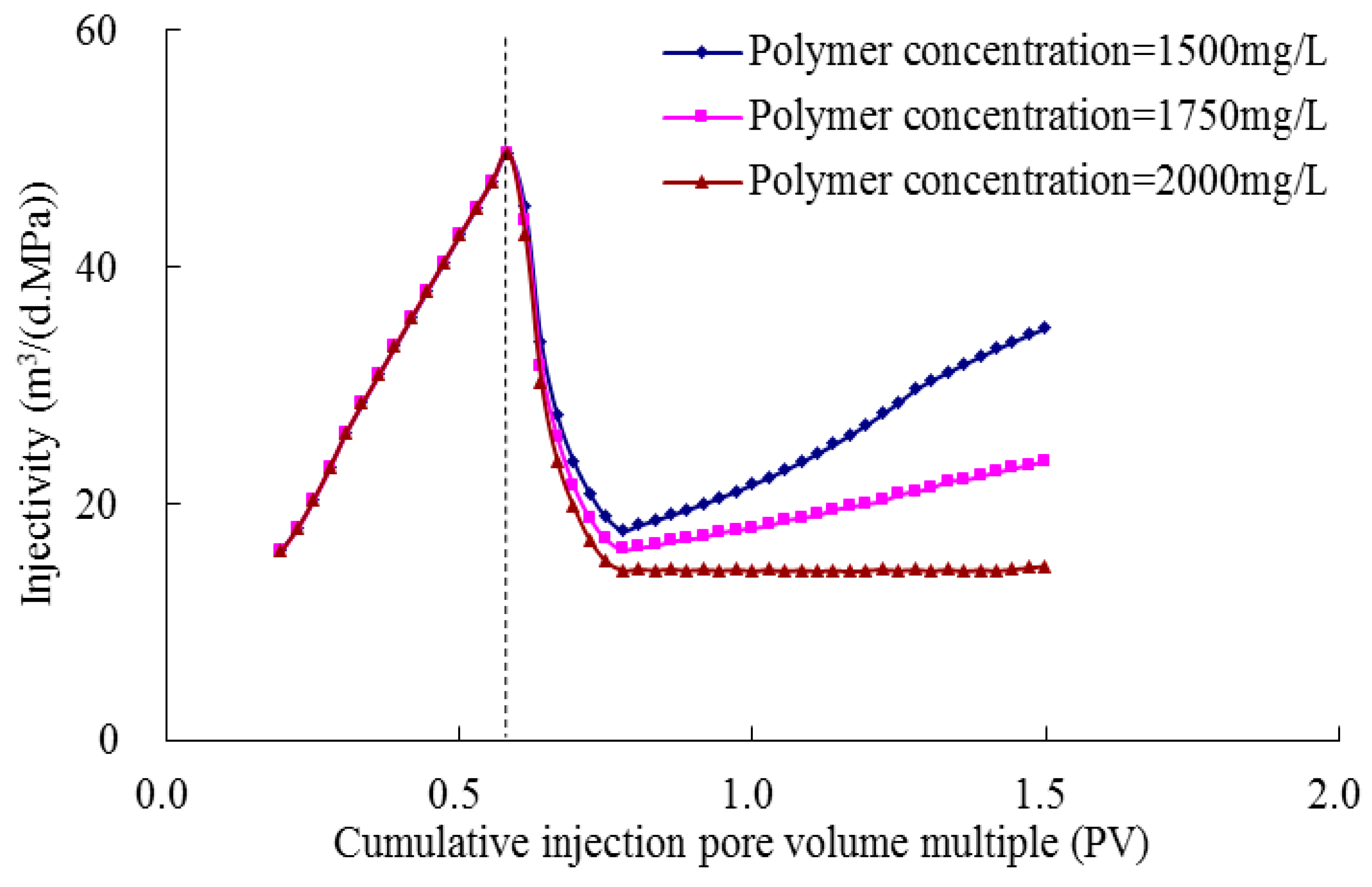
Figure 13 indicates that when the polymer concentration is 1500 mg/L, 1750 mg/L, and 2000 mg/L, the injectivity respectively decreases by 64%, 67%, and 71% before polymer breakthrough, and increases by 96%, 46%, and 2% after polymer breakthrough. It can be seen that the higher the polymer concentration, the more the injectivity decreases before polymer breakthrough, and the less the injectivity increases after polymer breakthrough.
5. Conclusions
On the basis of polymer–oil fractional flow theory and the equivalent seepage resistance method, we proposed a semi-analytical model that evaluates the commingle and zonal injectivity for an offshore multilayer reservoir according to the concept “based on the fluid dynamic characteristics from every frontal saturation between injector and producer” by dividing the entire flow region into interrelated parts. This model needs less manpower, and also can provide a reference for the optimization of polymer flood injection parameters for EOR operations.
The proposed model takes into account both polymer rheology effects and the two-phase flow resistance coefficient. Compared with the linear core floods that suffer from steady-state conditions through the core, the proposed model improves the calculation accuracy of pressure drop and polymer injectivity through consideration of an actual well injection situation where both pressure and shear forces are nonlinear gradients.
In the primary water flooding phase, the IPPD decreases and the CI increases gradually due to low water viscosity and small seepage resistance. In the secondary polymer flooding phase, before polymer breakthrough, the mobility control effect of polymer solution result in a rapid increase of IPPD and a decrease of CI by 76%; after polymer breakthrough, the IPPD decreases gradually while the CI increases by 17%. In the subsequent water flooding phase, the injected water further reduces the viscosity of the displacement fluid; thus, the IPPD decreases rapidly, and the CI increases until it stabilizes.
The change law of zonal injectivity is consistent with that of CI. During polymer flooding, the polymer solution preferentially enters into the high-K layer. The high seepage resistance slows down the fluid advance velocity and leads to the decrease of the injection rate, which forces the reinjected polymer to enter into the low-K layer and increases the flow rate. The injectivity of the high-K layer and the low-K layer decrease by 80% and 55% respectively before polymer breakthrough, and increase by 13% and 28% respectively after polymer breakthrough.
The higher the injection rate and the lower the polymer concentration, the better the injectivity is before polymer breakthrough. An earlier injection time, lower injection rate, larger polymer injection volume, and lower polymer concentration will improve the injectivity after polymer breakthrough. The polymer breakthrough time is a significant indicator in polymer flood optimization.
Author Contributions
Conceptualization, L.S.; Data curation, Y.J.; Formal analysis, L.S.; Funding acquisition, Y.L.; Methodology, L.S. and Y.J.; Project administration, H.J.; Supervision, B.L.; Validation, L.S. and Y.J.; Writing–review & editing, Y.L.
Funding
This research was founded by the National Natural Science Foundation of China, grant number 2017ZX05030-001.
Acknowledgments
The authors are grateful for the technical and financial support from the Research Institute of Petroleum Exploration and Development, Petrochina, Beijing 100083, China.
Conflicts of Interest
The authors declare no conflict of interest.
References
- Mogbo, O.C. Polymer flood simulation in a heavy oil field: Offshore Niger-delta experience. In Proceedings of the SPE Enhanced Oil Recovery Conference, Kuala Lumpur, Malaysia, 19–21 July 2011. [Google Scholar]
- Ma, K.Q.; Li, Y.L.; Wang, L.L.; Zhu, X.L. Practice of the early stage polymer flooding on LD offshore oilfield in Bohai bay of China. In Proceedings of the SPE Asia Pacific Enhanced Oil Recovery Conference, Kuala Lumpur, Malaysia, 11–13 August 2015. [Google Scholar]
- Morel, D.C.; Vert, M.; Jouenne, S.; Gauchet, R.; Bouger, Y. First polymer injection in deep offshore field Angola: Recent advances in the Dalia/Camelia field case. In Proceedings of the SPE Annual Technical Conference and Exhibition, Florence, Italy, 19–22 September 2010. [Google Scholar]
- Liu, R.; Jiang, H.Q.; Zhang, X.S. Effective characteristics of early polymer flooding in mid-to-low viscosity offshore reservoir. Acta Pet. Sin. 2010, 31, 280–283. [Google Scholar]
- Kaminsky, R.D.; Wattenbarger, R.C.; Szafranski, R.C.; Coutee, A.S. Guidelines for polymer flooding evaluation and development. In Proceedings of the International Petroleum Technology Conference, Dubai, UAE, 4–6 December 2007. [Google Scholar]
- Kang, X.D.; Zhang, J.; Sun, F.J.; Zhang, F.J.; Feng, G.Z.; Yang, J.R.; Zhang, X.S.; Xiang, W.T. A review of polymer EOR on offshore heavy oil field in Bohai Bay, China. In Proceedings of the SPE Enhanced Oil Recovery Conference, Kuala Lumpur, Malaysia, 19–21 July 2011. [Google Scholar]
- Cao, B.G.; Luo, P.Y. An experimental study on rheological properties of the associating polymer solution in porous medium. Acta Pet. Sin. 2011, 32, 652–657. [Google Scholar]
- Jiang, W.D.; Kang, X.D.; Xie, K.; Lu, X.G. Degree of the association of hydrophobically associating polymer and its adaptability to the oil reservoir. Pet. Geol. Oilfield Dev. Daqing 2013, 32, 103–107. [Google Scholar]
- Ren, K.; Jiang, G.Y.; Xu, C.M.; Lin, M.Y.; Luo, M.Q. Solution conformation of hydrophobically associating polymers. J. Univ. Pet. China 2005, 29, 117–120. [Google Scholar]
- Taylor, K.C.; Nasr-El-Din, H.A. Hydrophobically associating polymers for oil field applications. In Proceedings of the Canadian International Petroleum Conference, Calgary, AB, Canada, 12–14 June 2007. [Google Scholar]
- Xie, X.Q.; Zhang, X.S.; Feng, G.Z.; He, C.B. Analysis on injection pressure of polymer flooding: A case study from a oilfield in Bohai Sea. Fault-Block Oil Gas Field 2012, 19, 195–198. [Google Scholar]
- Xie, K.; Lu, X.G.; Li, Q.; Jiang, W.D.; Yu, Q. Analysis of reservoir applicability of hydrophobically associating polymer. SPE J. 2016, 21, 1–9. [Google Scholar] [CrossRef]
- Lake, L.W. Enhanced Oil Recovery; Prentice Hall: Upper Saddle River, NJ, USA, 1989; pp. 332–338. [Google Scholar]
- Seright, R.S. The effects of mechanical degradation and viscoelastic behavior on injectivity of polyacrylamide solutions. SPE J. 1983, 23, 475–485. [Google Scholar] [CrossRef]
- Shuler, P.J.; Kuehne, D.L.; Uhl, J.T.; Walkup, G.W., Jr. Improving polymer injectivity at west coyote field, California. SPE Reserv. Eng. 1987, 2, 271–280. [Google Scholar] [CrossRef]
- Buell, R.S.; Kazemi, H.; Poettmann, F.H. Analyzing injectivity of polymer solutions with the Hall plot. SPE Reserv. Eng. 1990, 5, 41–46. [Google Scholar] [CrossRef]
- Buell, R.S. Analyzing Injectivity of Non-Newtonian Fluids: An Application of the Hall Plot; Arthur Lakes Library, Colorado School of Mines: Golden, CO, USA, 1986. [Google Scholar]
- Liu, M.M.; Jiang, R.Z.; Xing, Y.C.; Yu, C.C.; He, W. Research on the injectivity of polymer solution. In Proceedings of the 13th National Congress on Hydrodynamics & 26th National Conference on Hydrodynamics, Qingdao, Shandong, China, 22–27 August 2014; pp. 879–887. [Google Scholar]
- AlSofi, A.M.; Blunt, M.J. Control of numerical dispersion in streamline-based simulations of augmented waterflooding. SPE J. 2013, 18, 1102–1111. [Google Scholar] [CrossRef]
- AlSofi, A.M.; Blunt, M.J. Streamline-based simulation of non-Newtonian polymer flooding. SPE J. 2010, 15, 895–905. [Google Scholar] [CrossRef]
- Jain, L.; Lake, L.W. Surveillance of secondary and tertiary floods: Application of Koval’s theory to isothermal enhanced oil recovery displacement. In Proceedings of the SPE Improved Oil Recovery Symposium, Tulsa, OK, USA, 12–16 April 2014. [Google Scholar]
- Koval, E.J. A method for predicting the performance of unstable miscible displacement in heterogeneous media. SPE J. 1963, 3, 145–154. [Google Scholar] [CrossRef]
- Seright, R.S. How much polymer should be injected during a polymer flood? In Proceedings of the SPE Improved Oil Recovery Conference, Tulsa, OK, USA, 11–13 April 2016. [Google Scholar]
- Luo, H.; Li, Z.; Tagavifar, M.; Lashgari, H.; Zhao, B.C.; Delshad, M.; Pope, G.A.; Mohanty, K.K. Modeling polymer flooding with crossflow in layered reservoirs considering viscous fingering. In Proceedings of the SPE Canada Heavy Oil Technical Conference, Calgary, AB, Canada, 15–16 February 2017. [Google Scholar]
- Lu, X.A.; Liu, F.; Liu, G.W.; Pei, Y.L.; Jiang, H.Q.; Chen, J.S. A polymer injectivity model establishment and application for early polymer injection. Arab. J. Sci. Eng. 2018, 43, 2625–2632. [Google Scholar] [CrossRef]
- Zhang, F.J. The optimum early polymer injection time for offshore heavy oil reservoir. China Offshore Oil Gas 2018, 30, 89–94. [Google Scholar]
- Wang, J.M.; Chen, G.; Li, Y.; Ma, M.R. A kinetic mechanism study on oil bank forming during polymer flooding. Pet. Geol. Oilfield Dev. Daqing 2007, 26, 64–66. [Google Scholar]
Figure 1.
Physical model of polymer flooding in a well pattern (I: Polymer single-phase flow region; II: Oil bank; III: Water–oil two-phase flow region; IV: Oil drainage region).
Figure 1.
Physical model of polymer flooding in a well pattern (I: Polymer single-phase flow region; II: Oil bank; III: Water–oil two-phase flow region; IV: Oil drainage region).
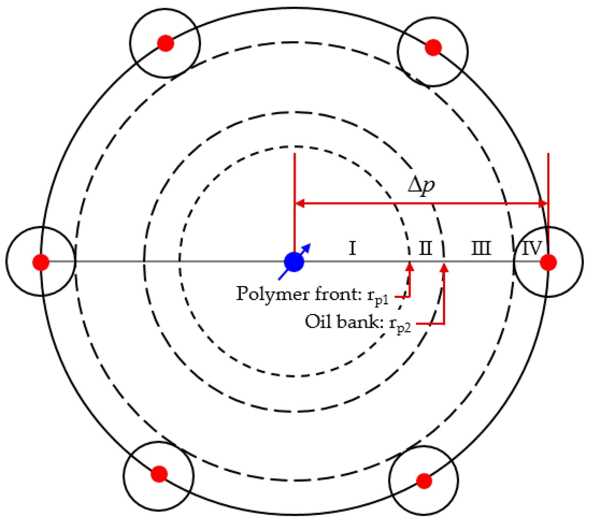
Figure 2.
Fractional flow curves of water flooding and polymer flooding.
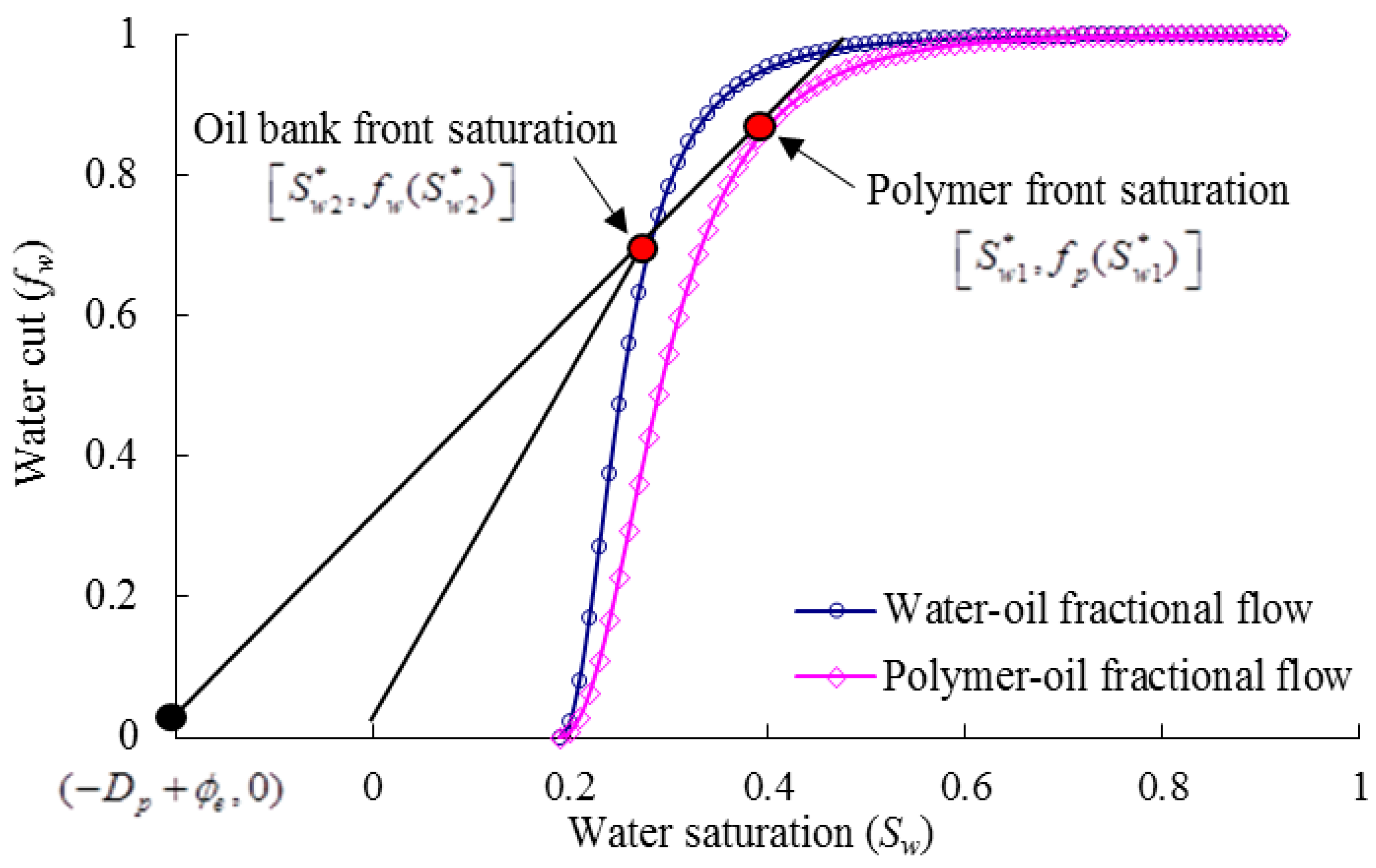
Figure 3.
Fluid saturation distribution during polymer flooding.
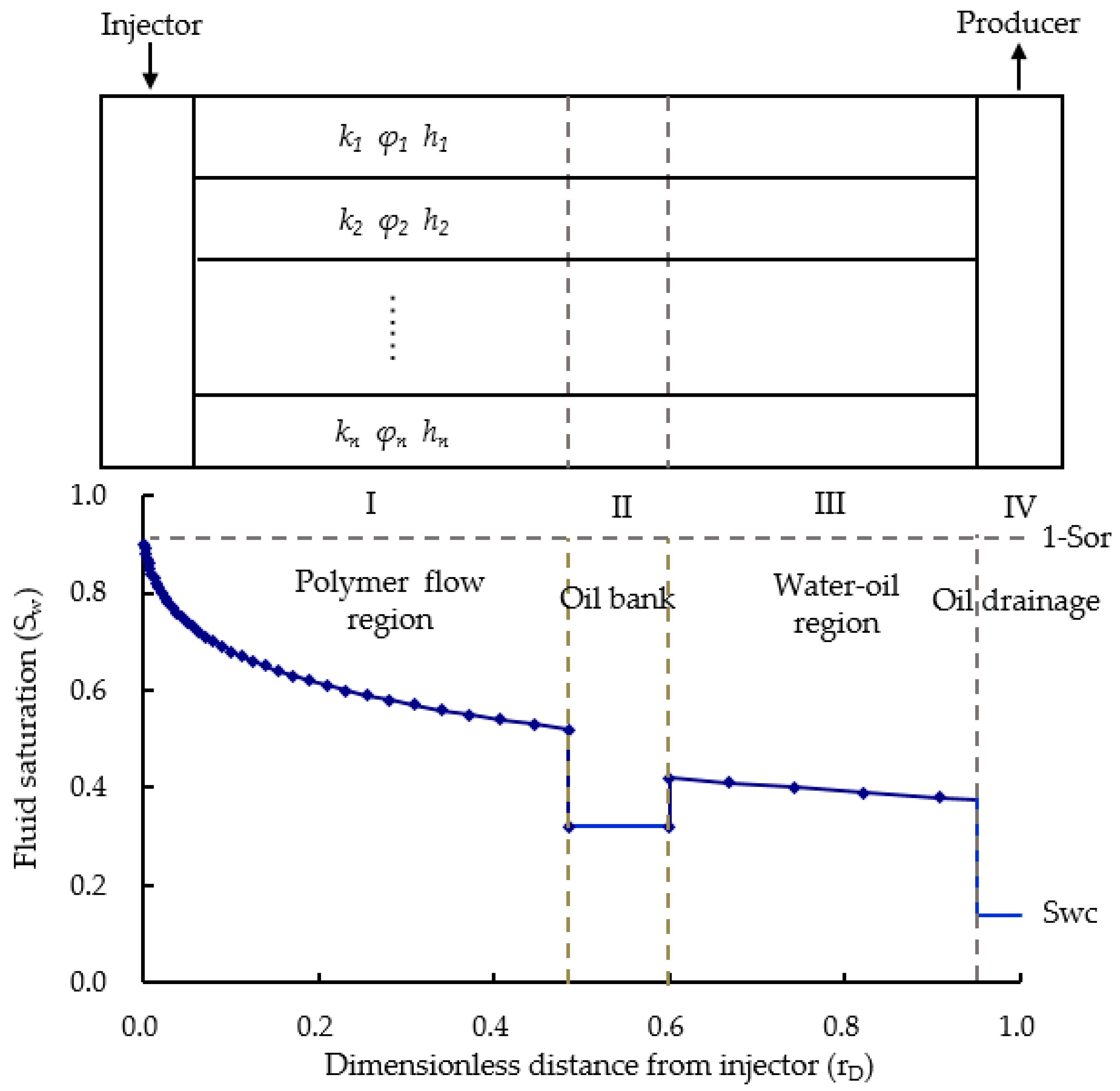
Figure 4.
Experiment process diagram.

Figure 5.
Comparison of flow rate ratio of No. 1 to No. 2 sand pack between observed and calculated results.
Figure 5.
Comparison of flow rate ratio of No. 1 to No. 2 sand pack between observed and calculated results.
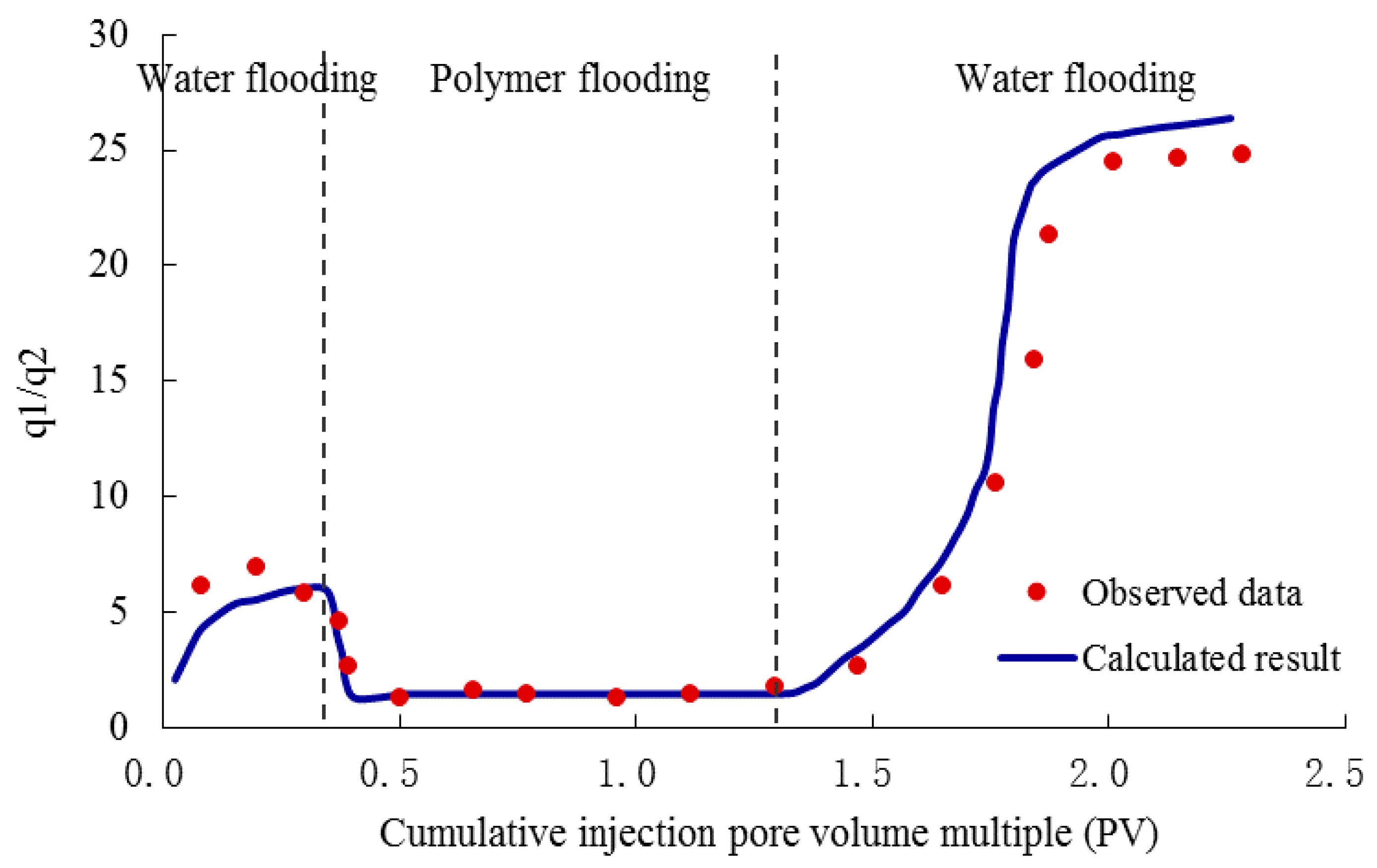
Figure 6.
Comparison of pressure drop between observed and calculated results.
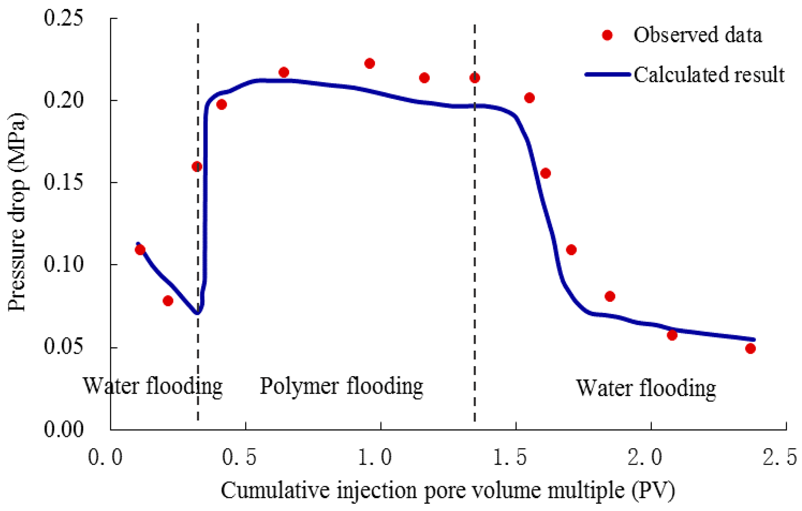
Figure 7.
Change law of pressure difference and commingled injectivity at different stages.
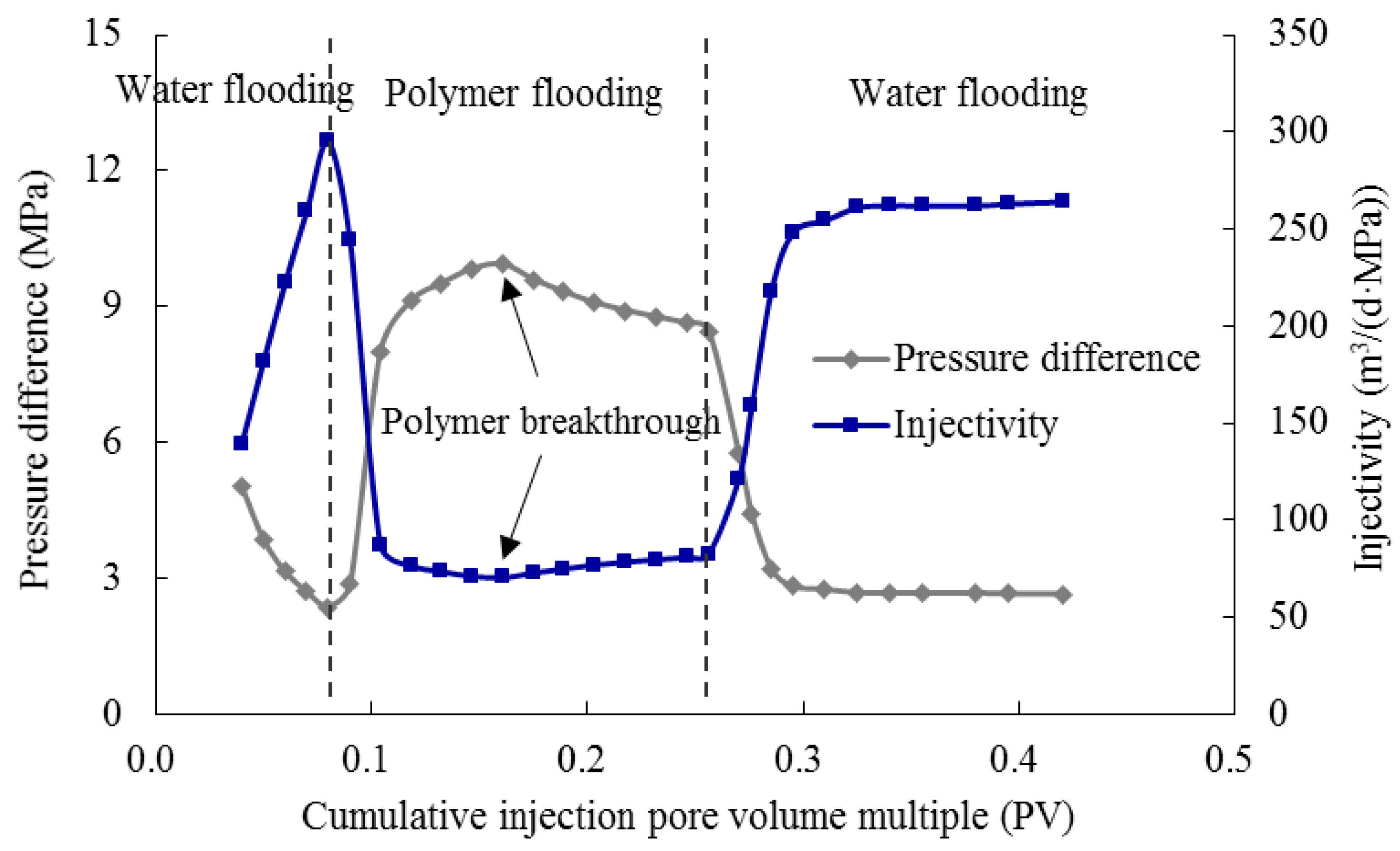
Figure 8.
Change law of the zonal flow rate at different stages.
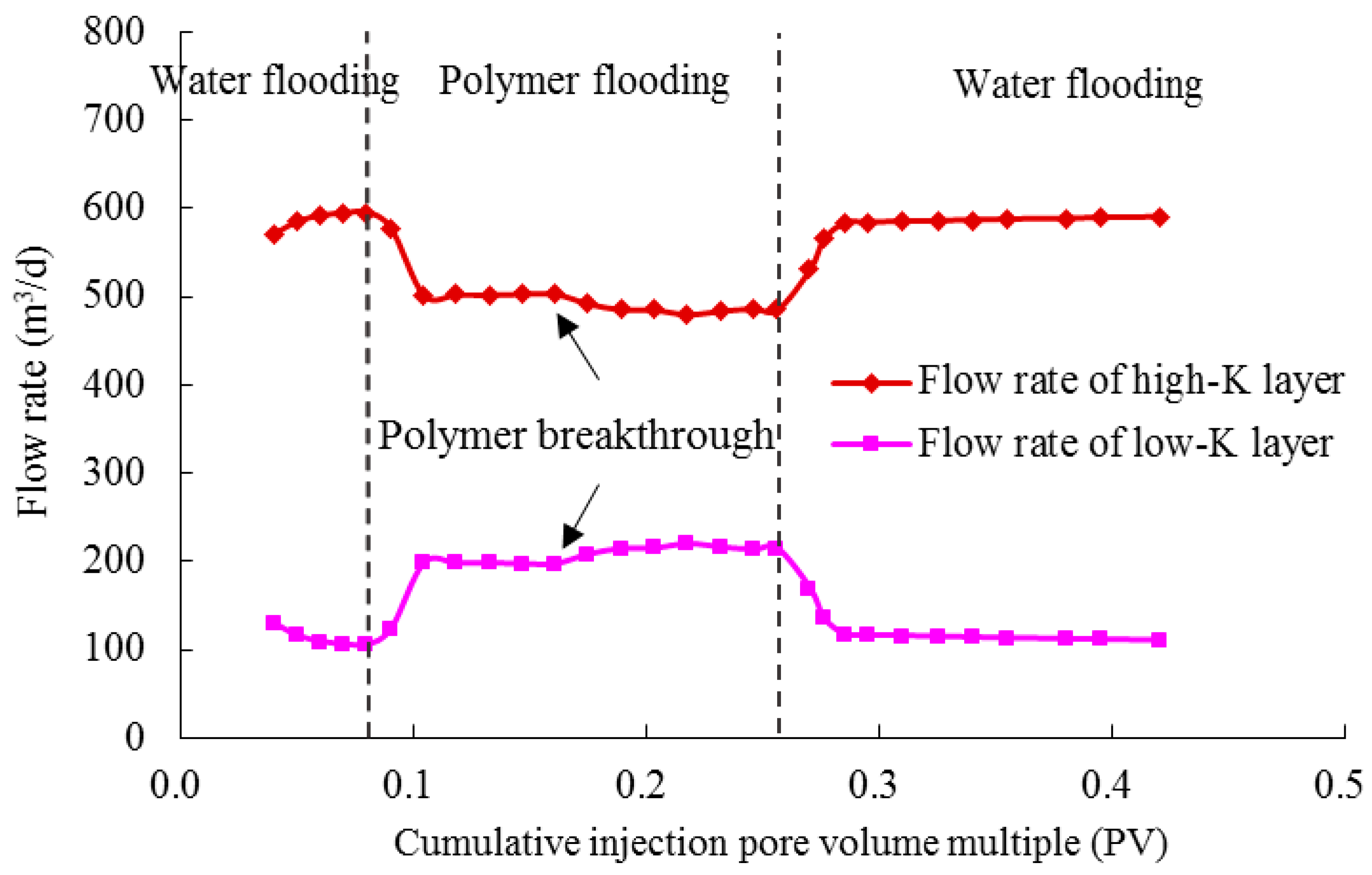
Figure 9.
Change law of zonal injectivity at different stages.
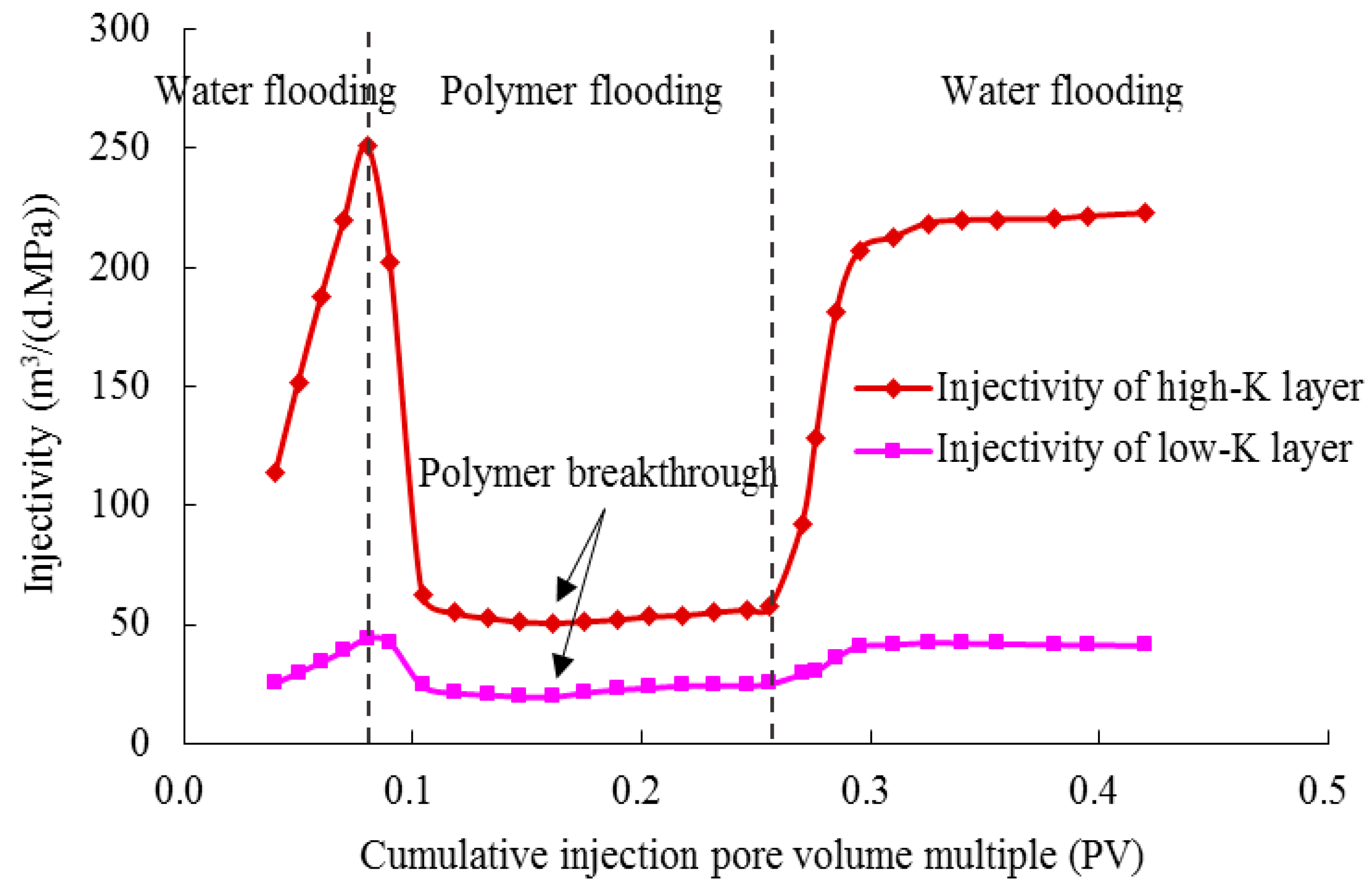
Figure 10.
The influence of polymer injection time on injectivity.

Figure 11.
The influence of polymer injection rate on injectivity.
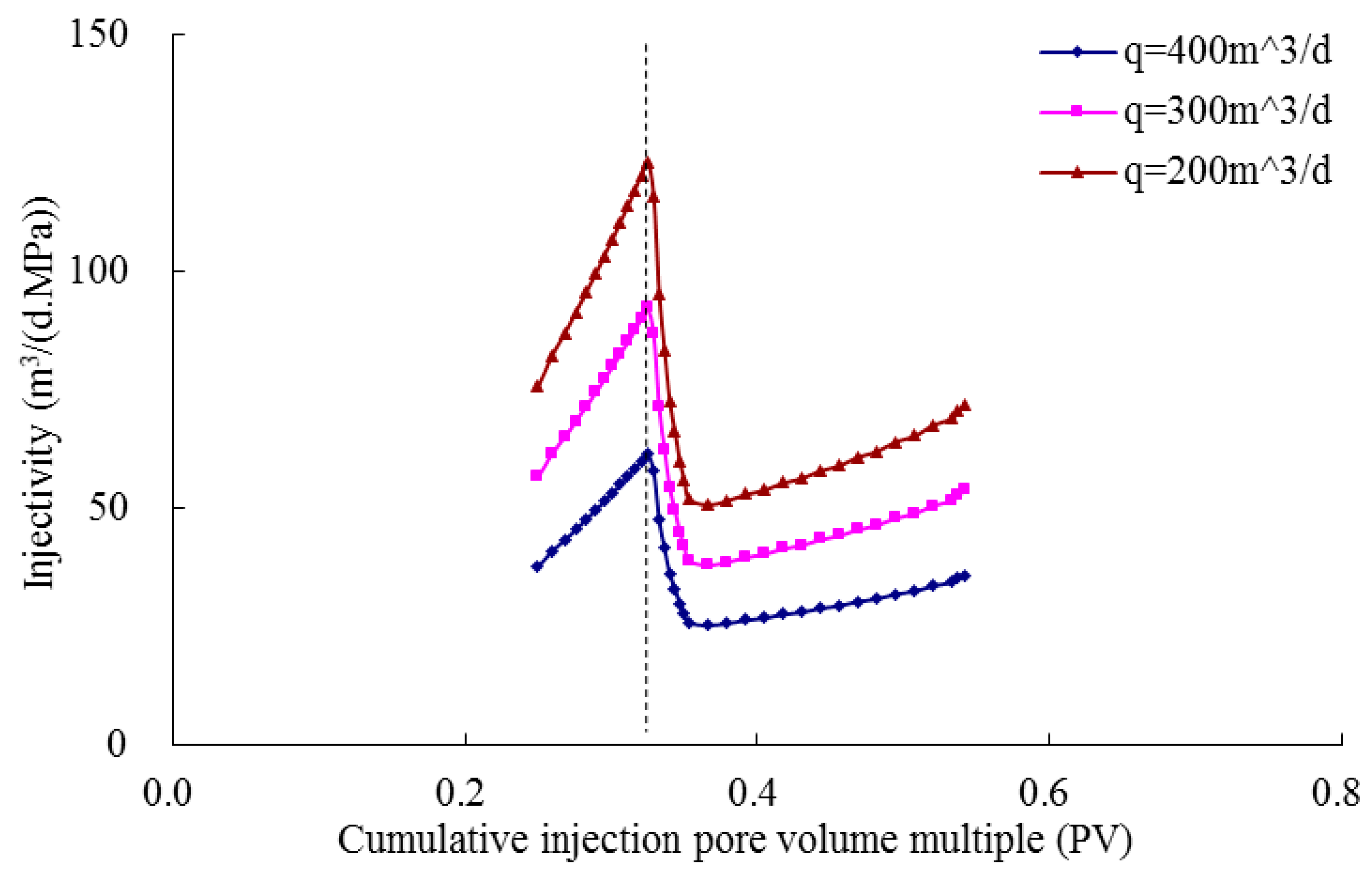
Figure 12.
The influence of polymer injection volume on injectivity.
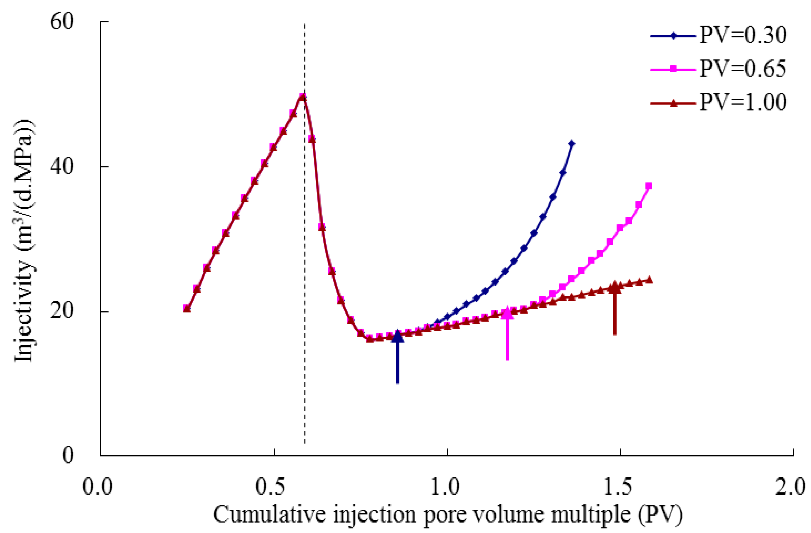
Figure 13.
The influence of polymer concentration on injectivity.

Table 1.
Basic parameters of injectivity verification.
| Items | Value | |
|---|---|---|
| Core parameters (Units) | Length of No. 1 sand pack (cm) | 30 |
| Diameter of No. 1 sand pack (cm) | 2.5 | |
| Permeability of No. 1 sand pack (10−3 µm2) | 4023 | |
| Porosity of No. 1 sand pack (%) | 30 | |
| Length of No. 2 sand pack (cm) | 30 | |
| Diameter of No. 2 sand pack (cm) | 2.5 | |
| Permeability of No. 2 sand pack (10−3 µm2) | 1962 | |
| Porosity of No. 2 sand pack (%) | 28 | |
| Fluid parameters (Units) | Oil viscosity (mPa·s) | 70 |
| Water viscosity (mPa·s) | 0.49 | |
| Water salinity (mg/L) | 5855 | |
| Polymer viscosity (mPa·s) | 8 | |
| Polymer concentration (mg/L) | 1750 | |
| Pow law exponent (–) | 0.336 | |
| Inaccessible pore volume (–) | 0.18 | |
| Experiment parameters (Units) | Reservoir temperature (K) | 338 |
| Injection flow rate (cm3/min) | 1 | |
| Cumulative injected water volume in primary water flooding (PV) | 0.3 | |
| Cumulative injected polymer volume in secondary polymer flooding (PV) | 1.0 | |
| Cumulative injected polymer volume in subsequent water flooding (PV) | 1.0 | |
Table 2.
Basic parameters of semi-analytical model calculation.
| Items | Value | |
|---|---|---|
| Geology parameters (Units) | Porosity (%) | 29 |
| Thickness of 1st layer (m) | 20 | |
| Permeability of 1st layer (10−3 µm2) | 3800 | |
| Thickness of 2nd layer (m) | 18 | |
| Permeability of 2nd layer (10−3 µm2) | 1900 | |
| Fluid parameters (Units) | Oil viscosity (mPa·s) | 70 |
| Water viscosity (mPa·s) | 0.49 | |
| Polymer concentration (mg/L) | 1750 | |
| Polymer viscosity (mPa·s) | 8 | |
| Power law exponent | 0.336 | |
| Inaccessible pore volume (–) | 0.18 | |
| Production parameters (Units) | Well pattern (–) | Five-spot |
| Well spacing (m) | 365 | |
| Bottom hole radius (m) | 0.1 | |
| Injection rate (PV/a) | 0.03 | |
| Cumulative injected water volume in primary water flooding (PV) | 0.08 | |
| Cumulative injected polymer volume in secondary polymer flooding (PV) | 0.18 | |
| Cumulative injected polymer volume in subsequent water flooding (PV) | 0.16 | |
© 2019 by the authors. Licensee MDPI, Basel, Switzerland. This article is an open access article distributed under the terms and conditions of the Creative Commons Attribution (CC BY) license (http://creativecommons.org/licenses/by/4.0/).
Share and Cite
MDPI and ACS Style
Sun, L.; Li, B.; Jiang, H.; Li, Y.; Jiao, Y. An Injectivity Evaluation Model of Polymer Flooding in Offshore Multilayer Reservoir. Energies 2019, 12, 1444. https://doi.org/10.3390/en12081444
AMA Style
Sun L, Li B, Jiang H, Li Y, Jiao Y. An Injectivity Evaluation Model of Polymer Flooding in Offshore Multilayer Reservoir. Energies. 2019; 12(8):1444. https://doi.org/10.3390/en12081444
Chicago/Turabian StyleSun, Liang, Baozhu Li, Hanqiao Jiang, Yong Li, and Yuwei Jiao. 2019. "An Injectivity Evaluation Model of Polymer Flooding in Offshore Multilayer Reservoir" Energies 12, no. 8: 1444. https://doi.org/10.3390/en12081444
Note that from the first issue of 2016, this journal uses article numbers instead of page numbers. See further details here.